Buletinul ştiinţific al Universităţii Politehnica din ... · Buletinul ştiinţific al...

Buletinul ştiinţific al Universităţii

"Politehnica" din Timişoara. Seria electronică

şi telecomunicaţii.

Scientific Bulletin of the "Politehnica"

University of Timişoara. Transactions on

Electronics and Communications

Printed: ISSN 1583-3380, Online: ISSN 2344-4444

Vol. 60(74), No. 2, 2015

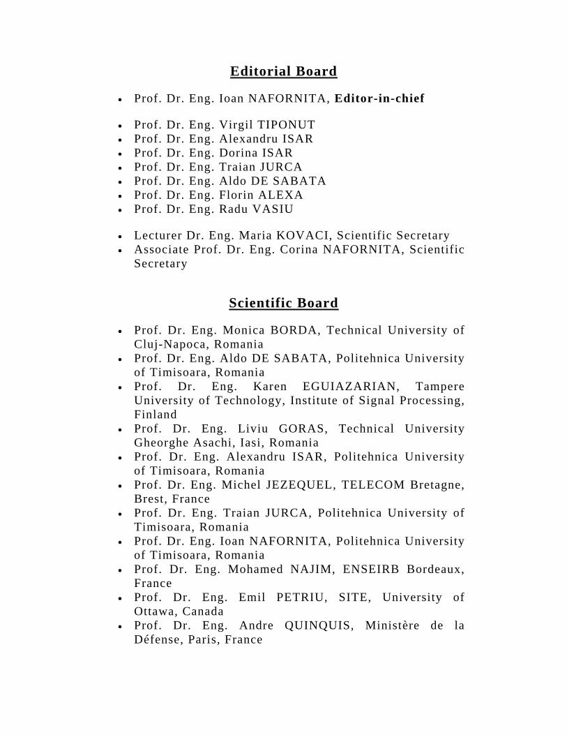
Editorial Board

• Prof. Dr. Eng. Ioan NAFORNITA, Editor-in-chief

• Prof. Dr. Eng. Virgil TIPONUT • Prof. Dr. Eng. Alexandru ISAR • Prof. Dr. Eng. Dorina ISAR • Prof. Dr. Eng. Traian JURCA • Prof. Dr. Eng. Aldo DE SABATA • Prof. Dr. Eng. Florin ALEXA • Prof. Dr. Eng. Radu VASIU

• Lecturer Dr. Eng. Maria KOVACI, Scientific Secretary • Associate Prof. Dr. Eng. Corina NAFORNITA, Scientific

Secretary

Scientific Board

• Prof. Dr. Eng. Monica BORDA, Technical University of Cluj-Napoca, Romania

• Prof. Dr. Eng. Aldo DE SABATA, Politehnica University of Timisoara, Romania

• Prof. Dr. Eng. Karen EGUIAZARIAN, Tampere University of Technology, Institute of Signal Processing, Finland

• Prof. Dr. Eng. Liviu GORAS, Technical University Gheorghe Asachi, Iasi, Romania

• Prof. Dr. Eng. Alexandru ISAR, Politehnica University of Timisoara, Romania

• Prof. Dr. Eng. Michel JEZEQUEL, TELECOM Bretagne, Brest, France

• Prof. Dr. Eng. Traian JURCA, Politehnica University of Timisoara, Romania

• Prof. Dr. Eng. Ioan NAFORNITA, Politehnica University of Timisoara, Romania

• Prof. Dr. Eng. Mohamed NAJIM, ENSEIRB Bordeaux, France

• Prof. Dr. Eng. Emil PETRIU, SITE, University of Ottawa, Canada

• Prof. Dr. Eng. Andre QUINQUIS, Ministère de la Défense, Paris, France

• Prof. Dr. Eng. Maria Victoria RODELLAR BIARGE, Polytechnic University of Madrid, Spain

• Prof. Dr. Eng. Alexandru SERBANESCU, Technical Military Academy, Bucharest, Romania

• Prof. Dr. Eng. Virgil TIPONUT, Politehnica University of Timisoara, Romania

• Prof. Dr. Eng. Radu VASIU, Politehnica University of Timisoara, Romania

Advisory Board

• Prof. Dr. Eng. Ioan NAFORNITA, Politehnica University of Timisoara, Romania

• Prof. Dr. Eng. Florin ALEXA, Politehnica University of Timisoara, Romania

• Prof. Dr. Eng. Monica BORDA, Technical University of Cluj-Napoca, Romania

• Prof. Dr. Eng. Alexandru ISAR, Politehnica University of Timisoara, Romania

• Prof. Dr. Eng. Radu VASIU, Politehnica University of Timisoara, Romania

Scientific Bulletinul of Politehnica University Timisoara

TRANSACTIONS on ELECTRONICS and COMMUNICATIONS

Volume 60(74), Issue 2, 2015

CONTENTS

Silvia V. Botea: "Analysis of the antenna circuit and its influence on the wheel unit’s RF performance"............................................................................................................................. 3 Camelia Loredana Ţeicu:

"Analysis of RF transceivers used in automotive"........................................................ 8 Cornel Balint, Aldo De Sabata, Septimiu Mischie:

"Ionospheric Propagation Investigation in Western Romania – An Experimental Approach"............................................................................................................................... 14 Ionel Petruţ, Marius Oteşteanu, Cornel Balint, Georgeta Budura:

"Cluster Capacity Increase through eICIC Technology – An Experimental Analysis".................................................................................................................................. 18

Bianca Enache, Marius Otesteanu, Daniel Tiuc:

"Review over different diagnostic specifications and testing tools used in automotive domain"................................................................................................................................... 22 Instructions for authors at the Scientific Bulletin of Politehnica University Timisoara - Transactions on Electronics and Communications ................................................................ 26

1

Scientific Bulletin of Politehnica University Timisoara


Volume 60(74), Issue 2, 2015

Analysis of the antenna circuit and its influence on the wheel unit’s RF performance

Silvia V. Botea 1

1 Faculty of Electronics and Telecommunications, Communications Dept. Bd. V. Parvan 2, 300223 Timisoara, Romania, e-mail [email protected]

Abstract – The purpose of this paper is to investigate the performance of the antenna used in the TiS (Tire Information System) module and to find a possible improved solution. A series of simulations of the loop antenna integrated in the TIS module is presented. There are considered 3 different cases: the standalone simulation of the module, the version where the module is placed on the rim, and the last one is the module simulated together with the rim and the tire. The position of the module on the rim and the influences of the tire based on the simulations results are presented by evaluating the impedance and the radiation efficiency. Different dimensions are considered for the rim and the tire. Keywords: TiS, antenna, HFSS

I. INTRODUCTION

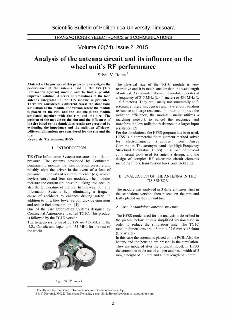
TiS (Tire Information System) measures the inflation pressure. The systems developed by Continental permanently monitor the tire's inflation pressure and reliably alert the driver in the event of a loss of pressure. It consists of a central receiver (e.g. remote keyless entry) and four rim modules. The modules measure the current tire pressure, taking into account also the temperature of the tire. In this way, our Tire Information Systems help eliminating a frequent cause of accidents to enhance driving safety. In addition to this, they lower carbon dioxide emissions and reduce fuel consumption. [1] One of the Tire Information Systems designed by Continental Automotive is called TG1C. This product is followed by the TG1D version. The frequencies required by TiS are 315 MHz in the U.S., Canada and Japan and 434 MHz for the rest of the world.

Fig. 1. TG1C product

The physical size of the TG1C module is very restrictive and it is much smaller than the wavelength of interest. As reminded above, the module operates at a frequency of 315 MHz (λ ~ 1 meter) or 434 MHz (λ ~ 0.7 meters). They are usually not structurally self-resonant at these frequencies and have a low radiation resistance and large reactance. In order to improve the radiation efficiency, the module usually utilizes a matching network to cancel the reactance and transform the low radiation resistance to a larger input resistance. [2] For the simulations, the HFSS program has been used. HFSS is a commercial finite element method solver for electromagnetic structures from Ansys Corporation. The acronym stands for High Frequency Structural Simulator (HFSS). It is one of several commercial tools used for antenna design, and the design of complex RF electronic circuit elements including filters, transmission lines, and packaging.

II. EVALUATION OF THE ANTENNA IN THE TIS SENSOR

The module was analyzed in 3 different cases: first in the standalone version, then placed on the rim and lastly placed on the rim and tire. A. Case 1: Standalone antenna structure

The HFSS model used for the analysis is described in the picture below. It is a simplified version used in order to reduce the simulation time. The TG1C module dimensions are: 48 mm x 27.6 mm x 12.5mm (L x W x H). In this case the antenna is placed on the PCB. Also the battery and the housing are present in the simulation. They are modeled after the physical model. In HFSS the antenna is made out of cooper and has a width of 5 mm, a height of 7.3 mm and a total length of 39 mm.

3

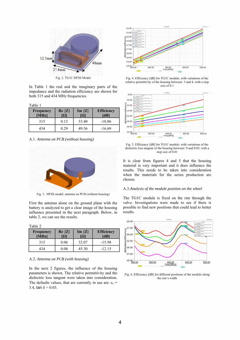
Fig. 2. TG1C HFSS Model

In Table 1 the real and the imaginary parts of the impedance and the radiation efficiency are shown for both 315 and 434 MHz frequencies. Table 1

Frequency [MHz]

Re Z [Ω]

Im Z [Ω]

Efficiency [dB]

315 0.13 33.40 -18.86

434 0.29 49.36 -16.69

A.1. Antenna on PCB (without housing)

Fig. 3. HFSS model: antenna on PCB (without housing)

First the antenna alone on the ground plane with the battery is analyzed to get a clear image of the housing influence presented in the next paragraph. Below, in table 2, we can see the results. Table 2

Frequency [MHz]

Re Z [Ω]

Im Z [Ω]

Efficiency [dB]

315 0.06 32.07 -15.98 434 0.08 45.30 -12.15

A.2. Antenna on PCB (with housing) In the next 2 figures, the influence of the housing parameters is shown. The relative permittivity and the dielectric loss tangent were taken into consideration. The defaults values, that are currently in use are: r = 3.4, tan = 0.03.

300.00 350.00 400.00 450.00 500.00Freq [MHz]

-19.50

-19.00

-18.50

-18.00

-17.50

-17.00

-16.50

-16.00

-15.50

-15.00

dB(R

adia

tionE

ffici

ency

)

HFSSDesign1XY Plot 4

315.0000434.0000

-18.8516

-19.0187-18.8734

-18.4732

-19.0352

-18.6374

-16.6877

-16.9398

-16.7751

-16.2960

-17.0180

-16.4790

119.0000

Curve InfodB(RadiationEff iciency)

Setup1 : Sw eep$rel_perm='3' Phi='0deg' Theta='0deg'

dB(RadiationEff iciency)Setup1 : Sw eep$rel_perm='3.2' Phi='0deg' Theta='0deg'




dB(RadiationEff iciency)Setup1 : Sw eep$rel_perm='4' Phi='0deg' Theta='0deg'

Fig. 4. Efficiency [dB] for TG1C module, with variations of the relative permittivity of the housing between: 3 and 4, with a step

size of 0.1

300.00 350.00 400.00 450.00 500.00Freq [MHz]

-22.00

-20.00

-18.00

-16.00

-14.00

-12.00

-10.00

-8.00

dB(R

adia

tionE

ffici

ency

)


315.0000434.0000

-19.9573

-16.0507

-17.1596

-18.0499

-18.7949

-19.4243

-18.2250

-12.0252

-14.1586

-15.5830

-16.6497

-17.5042

119.0000

Curve InfodB(RadiationEff iciency)

Setup1 : Sw eep$rel_perm='3.4' $tg_delta='0' Phi='0deg' Theta='0deg'

dB(RadiationEff iciency)Setup1 : Sw eep$rel_perm='3.4' $tg_delta='0.01' Phi='0deg' Theta='0deg'





Fig. 5. Efficiency [dB] for TG1C module, with variations of the dielectric loss tangent of the housing between: 0 and 0.05, with a

step size of 0.01

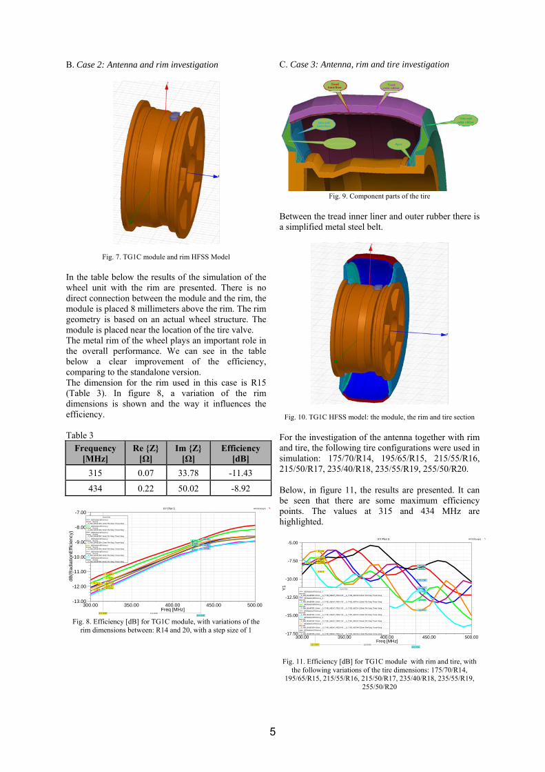
It is clear from figures 4 and 5 that the housing material is very important and it does influence the results. This needs to be taken into consideration when the materials for the series production are chosen. A.3.Analysis of the module position on the wheel The TG1C module is fixed on the rim through the valve. Investigations were made to see if there is possible to find new positions that could lead to better results.

300.00 350.00 400.00 450.00 500.00Freq [MHz]

-40.00

-37.50

-35.00

-32.50

-30.00

-27.50

-25.00

dB(R

adia

tionE

ffici

ency

)


315.0000434.0000

-28.6807

-29.6509-29.8561

-36.8071

-33.9666

-25.3478

-26.6242-26.9499

-33.4691

-30.2303

119.0000

Curve InfodB(RadiationEf ficiency)

Setup1 : Sw eep1Phi='0deg' Theta='0deg' var_y='-85mm' var_z='13mm'

dB(RadiationEf ficiency)Setup1 : Sw eep1Phi='0deg' Theta='0deg' var_y='-72mm' var_z='8mm'

dB(RadiationEf ficiency)Setup1 : Sw eep1Phi='0deg' Theta='0deg' var_y='-49mm' var_z='8mm'

dB(RadiationEf ficiency)Setup1 : Sw eep1Phi='0deg' Theta='0deg' var_y='2mm' var_z='-1mm'

dB(RadiationEf ficiency)Setup1 : Sw eep1Phi='0deg' Theta='0deg' var_y='25mm' var_z='15mm'

Fig. 6. Efficiency [dB] for different positions of the module along the rim’s width

4

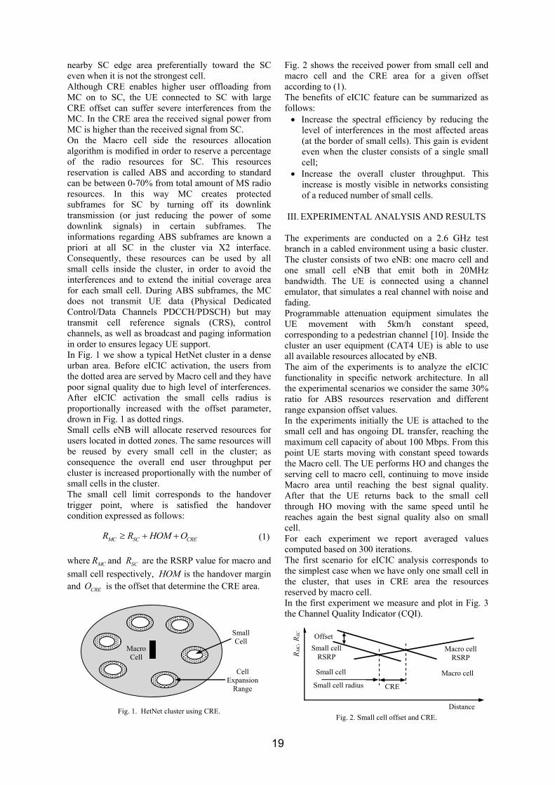
B. Case 2: Antenna and rim investigation

Fig. 7. TG1C module and rim HFSS Model

In the table below the results of the simulation of the wheel unit with the rim are presented. There is no direct connection between the module and the rim, the module is placed 8 millimeters above the rim. The rim geometry is based on an actual wheel structure. The module is placed near the location of the tire valve. The metal rim of the wheel plays an important role in the overall performance. We can see in the table below a clear improvement of the efficiency, comparing to the standalone version. The dimension for the rim used in this case is R15 (Table 3). In figure 8, a variation of the rim dimensions is shown and the way it influences the efficiency. Table 3

Frequency [MHz]

Re Z [Ω]

Im Z [Ω]

Efficiency [dB]

315 0.07 33.78 -11.43

434 0.22 50.02 -8.92

300.00 350.00 400.00 450.00 500.00Freq [MHz]

-13.00

-12.00

-11.00

-10.00

-9.00

-8.00

-7.00

dB(R

adia

tionE

ffici

ency

)


315.0000434.0000

-11.1892

-11.4378

-11.7514-11.7975-11.9742-12.1413

-12.2338

-8.8120-8.9266

-9.2184-9.1069-9.2421

-9.4590-9.5243

119.0000

Curve InfodB(RadiationEfficiency)

Setup1 : Sw eep__G_RIM_DIAMETER='14mm' Phi='0deg' Theta='0deg'

dB(RadiationEfficiency)Setup1 : Sw eep__G_RIM_DIAMETER='15mm' Phi='0deg' Theta='0deg'






Fig. 8. Efficiency [dB] for TG1C module, with variations of the

rim dimensions between: R14 and 20, with a step size of 1

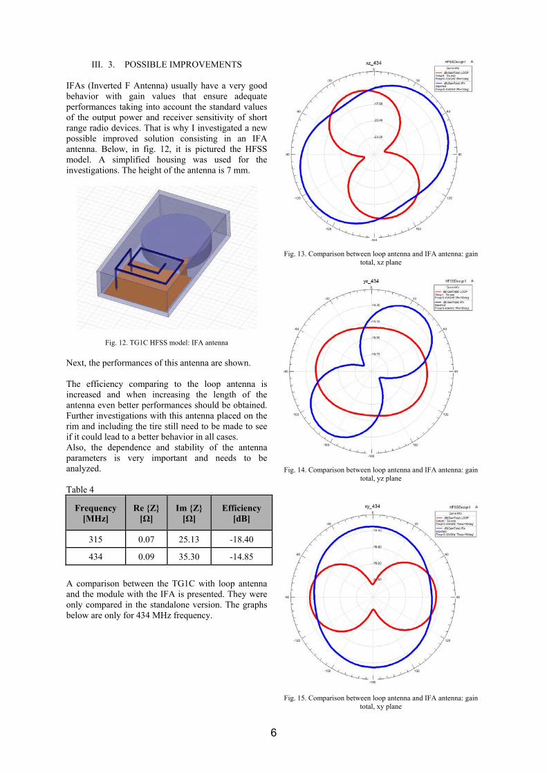
C. Case 3: Antenna, rim and tire investigation

Fig. 9. Component parts of the tire

Between the tread inner liner and outer rubber there is a simplified metal steel belt.

Fig. 10. TG1C HFSS model: the module, the rim and tire section For the investigation of the antenna together with rim and tire, the following tire configurations were used in simulation: 175/70/R14, 195/65/R15, 215/55/R16, 215/50/R17, 235/40/R18, 235/55/R19, 255/50/R20. Below, in figure 11, the results are presented. It can be seen that there are some maximum efficiency points. The values at 315 and 434 MHz are highlighted.

300.00 350.00 400.00 450.00 500.00Freq [MHz]

-17.50

-15.00

-12.50

-10.00

-7.50

-5.00

Y1


315.0000434.0000

-7.7925-7.8377

-7.0883-7.4412

-9.0078

-6.1783

-7.7762-8.1758

-10.1739

-12.9164

-11.2597

-11.7405

-14.2921

-8.6037

119.0000

Curve InfodB(RadiationEfficiency)_2

Imported__G_RIM_DIAMETER='15mm' __G_TYRE_HEIGHT_PROC='65' __G_TYRE_WIDTH='195mm' Phi='0deg' Theta='0deg'

dB(RadiationEfficiency)_3Imported__G_RIM_DIAMETER='16mm' __G_TYRE_HEIGHT_PROC='55' __G_TYRE_WIDTH='215mm' Phi='0deg' Theta='0deg'






Fig. 11. Efficiency [dB] for TG1C module with rim and tire, with the following variations of the tire dimensions: 175/70/R14,

195/65/R15, 215/55/R16, 215/50/R17, 235/40/R18, 235/55/R19, 255/50/R20

5

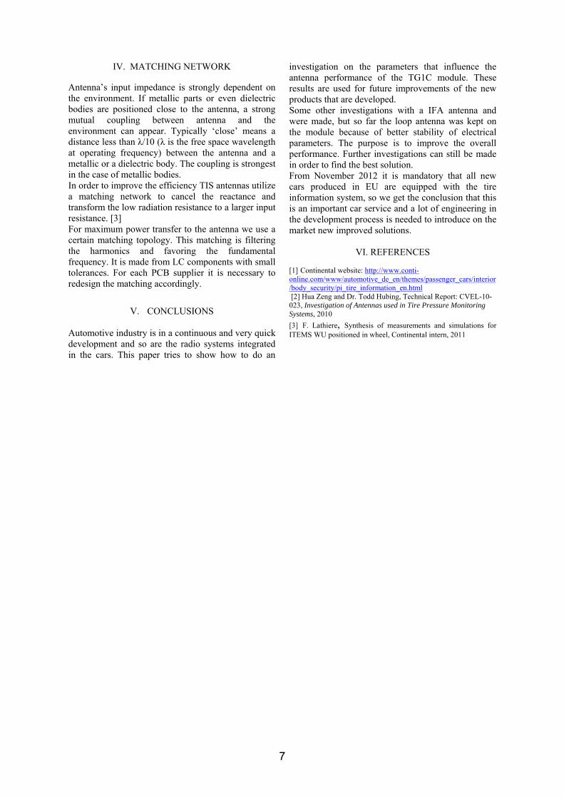
III. 3. POSSIBLE IMPROVEMENTS IFAs (Inverted F Antenna) usually have a very good behavior with gain values that ensure adequate performances taking into account the standard values of the output power and receiver sensitivity of short range radio devices. That is why I investigated a new possible improved solution consisting in an IFA antenna. Below, in fig. 12, it is pictured the HFSS model. A simplified housing was used for the investigations. The height of the antenna is 7 mm.

Fig. 12. TG1C HFSS model: IFA antenna

Next, the performances of this antenna are shown. The efficiency comparing to the loop antenna is increased and when increasing the length of the antenna even better performances should be obtained. Further investigations with this antenna placed on the rim and including the tire still need to be made to see if it could lead to a better behavior in all cases. Also, the dependence and stability of the antenna parameters is very important and needs to be analyzed. Table 4

Frequency [MHz]

Re Z [Ω]

Im Z [Ω]

Efficiency [dB]

315 0.07 25.13 -18.40

434 0.09 35.30 -14.85

A comparison between the TG1C with loop antenna and the module with the IFA is presented. They were only compared in the standalone version. The graphs below are only for 434 MHz frequency.

Fig. 13. Comparison between loop antenna and IFA antenna: gain total, xz plane

Fig. 14. Comparison between loop antenna and IFA antenna: gain total, yz plane

Fig. 15. Comparison between loop antenna and IFA antenna: gain total, xy plane

6

IV. MATCHING NETWORK Antenna’s input impedance is strongly dependent on the environment. If metallic parts or even dielectric bodies are positioned close to the antenna, a strong mutual coupling between antenna and the environment can appear. Typically ‘close’ means a distance less than λ/10 (λ is the free space wavelength at operating frequency) between the antenna and a metallic or a dielectric body. The coupling is strongest in the case of metallic bodies. In order to improve the efficiency TIS antennas utilize a matching network to cancel the reactance and transform the low radiation resistance to a larger input resistance. [3] For maximum power transfer to the antenna we use a certain matching topology. This matching is filtering the harmonics and favoring the fundamental frequency. It is made from LC components with small tolerances. For each PCB supplier it is necessary to redesign the matching accordingly.

V. CONCLUSIONS Automotive industry is in a continuous and very quick development and so are the radio systems integrated in the cars. This paper tries to show how to do an

investigation on the parameters that influence the antenna performance of the TG1C module. These results are used for future improvements of the new products that are developed. Some other investigations with a IFA antenna and were made, but so far the loop antenna was kept on the module because of better stability of electrical parameters. The purpose is to improve the overall performance. Further investigations can still be made in order to find the best solution. From November 2012 it is mandatory that all new cars produced in EU are equipped with the tire information system, so we get the conclusion that this is an important car service and a lot of engineering in the development process is needed to introduce on the market new improved solutions.

VI. REFERENCES [1] Continental website: http://www.conti-online.com/www/automotive_de_en/themes/passenger_cars/interior/body_security/pi_tire_information_en.html [2] Hua Zeng and Dr. Todd Hubing, Technical Report: CVEL-10-023, Investigation of Antennas used in Tire Pressure Monitoring Systems, 2010 [3] F. Lathiere, Synthesis of measurements and simulations for ITEMS WU positioned in wheel, Continental intern, 2011

7



Volume 60(74), Issue 2, 2015

Analysis of RF transceivers used in automotive

Camelia Loredana Ţeicu1

1 Faculty of Electronics and Telecommunications, Communications Dept. Bd. V. Parvan 2, 300223 Timisoara, Romania, e-mail [email protected]

Abstract – The paper presents the redesign of a radio frequency (RF) front-end transceiver used in automotive as part of the remote keyless entry (RKE) and tire-pressure monitoring (TPMS) system. The redesign must keep the same RF performances or improve them in some cases. A practical impedance analysis is done to choose the best design in terms of performance versus costs for reception and transmission. Comparative measurements for the main characteristics, on the RF transceiver board, before and after the redesign, were realized to confirm the obtained performances. Keywords: RKE, TPMS, transceiver, SAW filter

I. INTRODUCTION

Short-range radio systems designed to work in unlicensed industrial, scientific, and medical (ISM) bands between 300MHz and 928MHz use as key components the low-cost FSK and/or ASK transceiver ICs. Applications for these short-range devices (SRDs) include remote keyless entry and tire-pressure monitoring systems. Remote keyless entry is very popular in the new vehicles, because beside the advantages for comfort this technology minimizes the risk of theft. The new generation of RKE systems is capable to inform the users what is the status of the vehicle: if the doors are not locked or if needs more gas. [1] The tire-pressure monitoring system (TPMS) is more and more requested by the automotive producers as well, because is increasing the safety of the driver and the efficiency of the driving. There are two types of TPM: indirect or direct. The direct TPM is more precise and easy to use than the indirect TPM, which is using the speed sensors from the anti-lock braking system (ABS). [2] A. RF transceiver

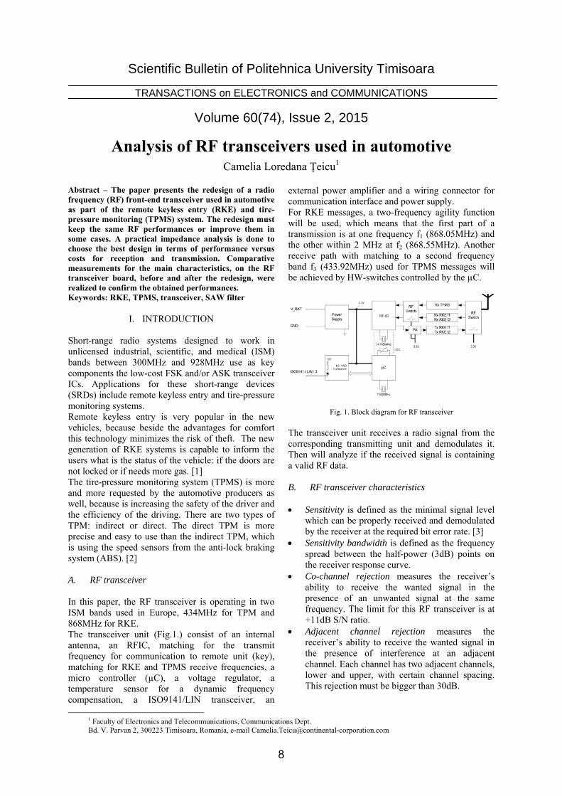
In this paper, the RF transceiver is operating in two ISM bands used in Europe, 434MHz for TPM and 868MHz for RKE. The transceiver unit (Fig.1.) consist of an internal antenna, an RFIC, matching for the transmit frequency for communication to remote unit (key), matching for RKE and TPMS receive frequencies, a micro controller (µC), a voltage regulator, a temperature sensor for a dynamic frequency compensation, a ISO9141/LIN transceiver, an

external power amplifier and a wiring connector for communication interface and power supply. For RKE messages, a two-frequency agility function will be used, which means that the first part of a transmission is at one frequency f1 (868.05MHz) and the other within 2 MHz at f2 (868.55MHz). Another receive path with matching to a second frequency band f3 (433.92MHz) used for TPMS messages will be achieved by HW-switches controlled by the µC.

Fig. 1. Block diagram for RF transceiver

The transceiver unit receives a radio signal from the corresponding transmitting unit and demodulates it. Then will analyze if the received signal is containing a valid RF data. B. RF transceiver characteristics

Sensitivity is defined as the minimal signal level

which can be properly received and demodulated by the receiver at the required bit error rate. [3]

Sensitivity bandwidth is defined as the frequency spread between the half-power (3dB) points on the receiver response curve.

Co-channel rejection measures the receiver’s ability to receive the wanted signal in the presence of an unwanted signal at the same frequency. The limit for this RF transceiver is at +11dB S/N ratio.

Adjacent channel rejection measures the receiver’s ability to receive the wanted signal in the presence of interference at an adjacent channel. Each channel has two adjacent channels, lower and upper, with certain channel spacing. This rejection must be bigger than 30dB.

8

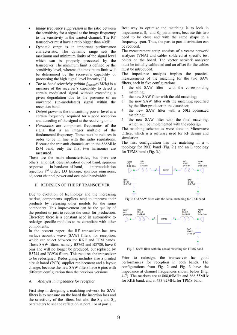
Image frequency suppression is the ratio between the sensitivity for a signal at the image frequency to the sensitivity in the wanted channel. The RF transceiver must have a ratio bigger than 40dB.

Dynamic range is an important performance characteristic. The dynamic range sets the maximum and minimum limits of the signal level which can be properly processed by the transceiver. The minimum limit is defined by the sensitivity level, whereas the maximum limit will be determined by the receiver’s capability of processing the high signal level linearity.[3]

The in-band selectivity (within fchannel±1MHz) is a measure of the receiver’s capability to detect a certain modulated signal without exceeding a given degradation due to the presence of an unwanted (un-modulated) signal within the reception band.

Output power is the transmitting power level at a certain frequency, required for a good reception and decoding of the signal at the receiving unit.

Harmonics are component frequencies of the signal that is an integer multiple of the fundamental frequency. These must be reduces in order to be in line with the radio regulations. Because the transmit channels are in the 868MHz ISM band, only the first two harmonics are measured.

These are the main characteristics, but there are others, amongst: desensitization out-of band, spurious response in-band/out-of-band, intermodulation rejection 3rd order, LO leakage, spurious emissions, adjacent channel power and occupied bandwidth.

II. REDESIGN OF THE RF TRANSCEIVER

Due to evolution of technology and the increasing market, components suppliers tend to improve their products by releasing other models for the same component. This improvement can be the quality of the product or just to reduce the costs for production. Therefore there is a constant need in automotive to redesign specific modules to be compliant with other components. In the present paper, the RF transceiver has two surface acoustic wave (SAW) filters, for reception, which can select between the RKE and TPM bands. These SAW filters, namely B3762 and B3780, have 8 pins and will no longer be produced, but replaced by B3744 and B3936 filters. This requires the transceiver to be redesigned. Redesigning includes also a printed circuit board (PCB) supplier replacement and a layout change, because the new SAW filters have 6 pins with different configuration than the previous versions. A. Analysis in impedance for reception

First step in designing a matching network for SAW filters is to measure on the board the insertion loss and the selectivity of the filters, but also the S11 and S22 parameters to see the reflection at port 1 or at port 2.

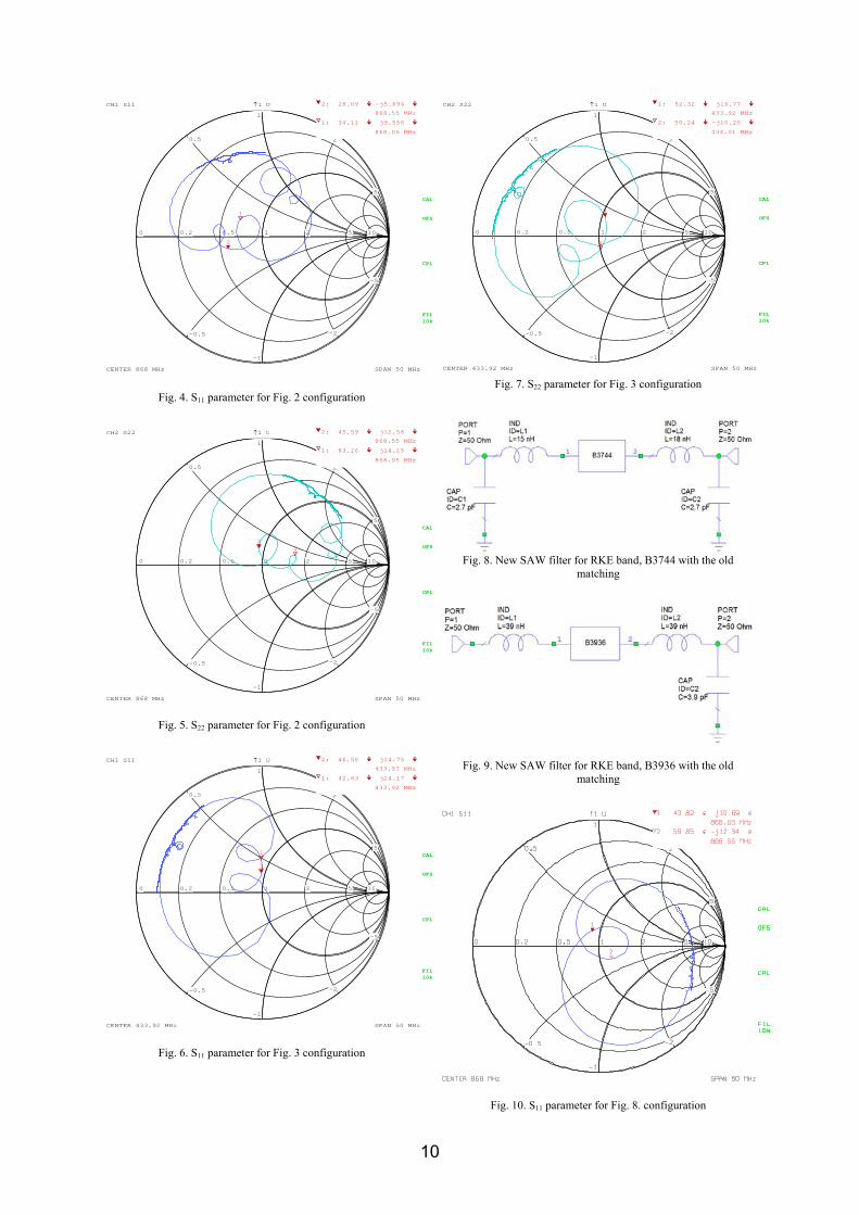
Best way to optimize the matching is to look in impedance at S11 and S22 parameters, because this two need to be close and with the same shape in a frequency span. Thus, the part to part distribution can be reduced. The measurement setup consists of a vector network analyzer (VNA) and cables soldered at specific test points on the board. The vector network analyzer must be initially calibrated and an offset for the cables must be introduced. The impedance analysis implies the practical measurements of the matching for the two SAW filters, each in five configurations: 1. the old SAW filter with the corresponding

matching; 2. the new SAW filter with the old matching; 3. the new SAW filter with the matching specified

by the filter producer in the datasheet; 4. the new SAW filter with a 50Ω optimized

matching; 5. the new SAW filter with the final matching,

which will be implemented with the redesign. The matching schematics were done in Microwave Office, which is a software used for RF design and simulation. The first configuration has the matching in a π topology for RKE band (Fig. 2.) and an L topology for TPMS band (Fig. 3.):

Fig. 2. Old SAW filter with the actual matching for RKE band

Fig. 3. SAW filter with the actual matching for TPMS band

Prior to redesign, the transceiver has good performances for reception in both bands. The configurations from Fig. 2 and Fig. 3 have the impedance at channel frequencies shown below (Fig. 4-7). The markers are at 868,05MHz and 868,55MHz for RKE band, and at 433,92MHz for TPMS band.

9

0 0.2 0.5 1 2 5 10

-5

-2

-1

-0.5

0.5

1

2

5

CH1 1 U

FIL10k10kFIL10k10k

CPL

OFS

CAL

CENTER 868 MHz SPAN 50 MHz

S11

1

2

2: 28.09 -j5.694

868.55 MHz

1: 34.11 j9.556

868.05 MHz

Fig. 4. S11 parameter for Fig. 2 configuration

0 0.2 0.5 1 2 5 10

-5

-2

-1

-0.5

0.5

1

2

5

CH2 1 U

CENTER 868 MHz SPAN 50 MHz

FIL10k10kFIL10k10k

CAL

CPL

OFS

S22

12

2: 45.59 j12.56

868.55 MHz

1: 83.26 j14.15

868.05 MHz


0 0.2 0.5 1 2 5 10

-5

-2

-1

-0.5

0.5

1

2

5

CH1 1 U

CENTER 433.92 MHz SPAN 50 MHz

FIL10k10kFIL10k10k

CPL

OFS

CAL

S11

1

2

2: 46.56 j14.75

433.97 MHz

1: 42.63 j24.17

433.92 MHz


0 0.2 0.5 1 2 5 10

-5

-2

-1

-0.5

0.5

1

2

5

CH2 1 U

CENTER 433.92 MHz SPAN 50 MHz

FIL10k10kFIL10k10k

CPL

OFS

CAL

S22

1

2

1: 52.32 j16.77

433.92 MHz

2: 50.24 -j10.25

434.01 MHz


Fig. 8. New SAW filter for RKE band, B3744 with the old

matching

Fig. 9. New SAW filter for RKE band, B3936 with the old matching

Fig. 10. S11 parameter for Fig. 8. configuration

10

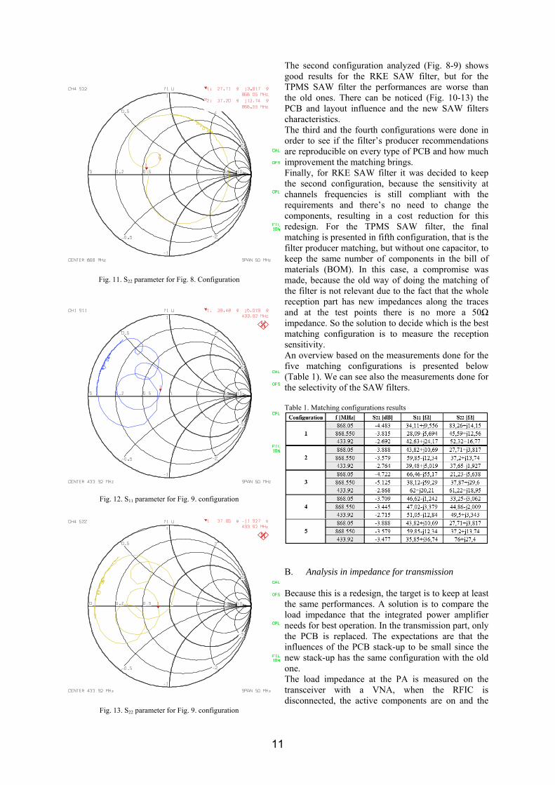
Fig. 11. S22 parameter for Fig. 8. Configuration



The second configuration analyzed (Fig. 8-9) shows good results for the RKE SAW filter, but for the TPMS SAW filter the performances are worse than the old ones. There can be noticed (Fig. 10-13) the PCB and layout influence and the new SAW filters characteristics. The third and the fourth configurations were done in order to see if the filter’s producer recommendations are reproducible on every type of PCB and how much improvement the matching brings. Finally, for RKE SAW filter it was decided to keep the second configuration, because the sensitivity at channels frequencies is still compliant with the requirements and there’s no need to change the components, resulting in a cost reduction for this redesign. For the TPMS SAW filter, the final matching is presented in fifth configuration, that is the filter producer matching, but without one capacitor, to keep the same number of components in the bill of materials (BOM). In this case, a compromise was made, because the old way of doing the matching of the filter is not relevant due to the fact that the whole reception part has new impedances along the traces and at the test points there is no more a 50Ω impedance. So the solution to decide which is the best matching configuration is to measure the reception sensitivity. An overview based on the measurements done for the five matching configurations is presented below (Table 1). We can see also the measurements done for the selectivity of the SAW filters. Table 1. Matching configurations results

B. Analysis in impedance for transmission

Because this is a redesign, the target is to keep at least the same performances. A solution is to compare the load impedance that the integrated power amplifier needs for best operation. In the transmission part, only the PCB is replaced. The expectations are that the influences of the PCB stack-up to be small since the new stack-up has the same configuration with the old one. The load impedance at the PA is measured on the transceiver with a VNA, when the RFIC is disconnected, the active components are on and the

11

HW-switch is controlled for transmission, which leads to a 50Ω termination instead of the antenna. Before the redesign, the load impedance measured at the integrated PA is 18,53 + j29,13Ω at 868.05MHz and 18,59 + j29,26Ω at 868.55MHz (Fig. 14).

0 0.2 0.5 1 2 5 10

-5

-2

-1

-0.5

0.5

1

2

5

CH1 1 U

FIL10k10kFIL10k10k

CPL

OFS

CAI

START 680 MHz STOP 1.2 GHz

M

12

1: 18.53 j29.13

868.05 MHz

2: 18.59 j29.26

868.55 MHz

Fig. 14. Load impedance at the integrated PA before redesign

After the redesign, the load impedance measured at the integrated PA is 20.74 + j27,5Ω at 868.05MHz and 20,79 + j27,66Ω at 868.55MHz (Fig. 15). The difference is small, only 2Ω in the real part. In this case, nothing else is modified in the matching. The transmitter characteristics will remain the same and the output power is already calibrated on the production line, by increasing the gain and power steps of the PA.

0 0.2 0.5 1 2 5 10

-5

-2

-1

-0.5

0.5

1

2

5

CH1 1 U

FIL10k10kFIL10k10k

CPL

OFS

CAI

START 680 MHz STOP 1.2 GHz

M

12

1: 20.74 j27.50

868.05 MHz

2: 20.79 j27.66

868.55 MHz

Fig. 15. Load impedance at the integrated PA after redesign

III. MAIN CHARACTERISTICS MEASUREMENTS

In this section, the main characteristics of the RF transceiver are measured to see if the RF performance is still compliant with the design before the redesign. For these measurements two boards were used to compare the results before and after redesign. But for

a design validation, more samples must be measured to see the part to part distribution, due to components tolerances and other small influences. A. Setup configuration

The setup (Fig. 16) must simulate the corresponding RKE remote unit and the TPMS sensor and also to provide the interference signal for the tests.

Fig. 16. Test setup configuration

The measurements involve the application of the RF signal at the 50Ω reference by disconnecting the antenna matching and inserting a coaxial cable. The transceiver is inside the shielded box, where it is powered with 12V and the response on the ISO9141 is monitored with the PC. The PC also commands the trigger box and all the generators. The RF parameters corresponding to every type of telegram are introduced with a specific application on the PC. The test setup is calibrated on each frequency, so the attenuation inserted by the cables can be correlated in the results. For output power and harmonics measurement a spectrum analyzer and a 20dB attenuator were included in the setup. B. Comparative results

The following main characteristics were measured with the setup presented above: sensitivity at center frequency for each channel, sensitivity bandwidth, image frequency suppression, adjacent channel rejection, co-channel rejection, in band selectivity, dynamic range, output power and harmonics. A summarized table is presented below (Table 2): Table 2. Comparison of measured characteristics before and after redesign

12

The measuring method is very important as it can have significant influence on the results. A short description of every measurement is explained below: Sensitivity at center frequency: the power level is

adjusted until the sensitivity limit is reached. Sensitivity bandwidth: the frequency will be

sweep in a 300 kHz span, with 5 kHz step. For each step the power level is adjusted until the sensitivity limit is reached. The frequency and power level are recorded.

Image frequency suppression: the same signal is applied at center frequency and at image frequency. The sensitivity is measured for each frequency and recorded. The difference between sensitivities is the image frequency suppression.

Adjacent channel rejection: the signal is set at center frequency fc and the FM interference is set first at fc-channel spacing and then at fc+channel spacing. The S/N is recorded.

Co-channel rejection: the signal is set at center frequency fc and the FM interference is set at same frequency. The S/N is recorded.

Selectivity in band fc±1MHz: the signal center frequency is set at channel frequency and the continuous wave (CW) interference is swept in a 2MHz span, with 25 kHz step. S/N is recorded.

Dynamic range: the signal set at center frequency will be increased from -120dBm to 0dBM with 10dB steps. The errors are recorded at each step.[4]

Output power and harmonics: the transceiver is put in transmitting mode, and the power level is measured with the spectrum analyzer.

Fig. 17. Selectivity in band for first RKE channel

Fig. 18. Selectivity in band for second RKE channel

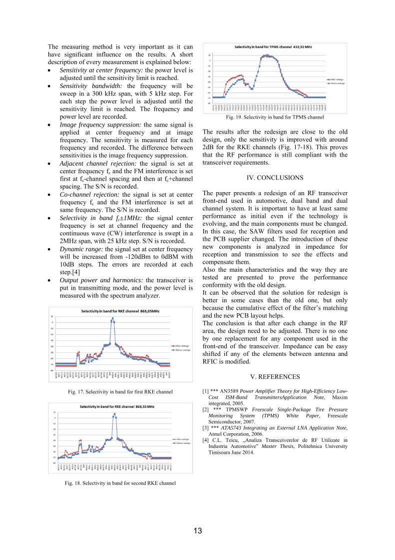
Fig. 19. Selectivity in band for TPMS channel

The results after the redesign are close to the old design, only the sensitivity is improved with around 2dB for the RKE channels (Fig. 17-18). This proves that the RF performance is still compliant with the transceiver requirements.

IV. CONCLUSIONS

The paper presents a redesign of an RF transceiver front-end used in automotive, dual band and dual channel system. It is important to have at least same performance as initial even if the technology is evolving, and the main components must be changed. In this case, the SAW filters used for reception and the PCB supplier changed. The introduction of these new components is analyzed in impedance for reception and transmission to see the effects and compensate them. Also the main characteristics and the way they are tested are presented to prove the performance conformity with the old design. It can be observed that the solution for redesign is better in some cases than the old one, but only because the cumulative effect of the filter’s matching and the new PCB layout helps. The conclusion is that after each change in the RF area, the design need to be adjusted. There is no one by one replacement for any component used in the front-end of the transceiver. Impedance can be easy shifted if any of the elements between antenna and RFIC is modified.

V. REFERENCES

[1] *** AN3589 Power Amplifier Theory for High-Efficiency Low-

Cost ISM-Band TransmittersApplication Note, Maxim integrated, 2005.

[2] *** TPMSWP Freescale Single-Package Tire Pressure Monitoring System (TPMS) White Paper, Freescale Semiconductor, 2007.

[3] *** ATA5743 Integrating an External LNA Application Note, Atmel Corporation, 2006.

[4] C.L. Teicu, „Analiza Transceiverelor de RF Utilizate in Industria Automotive” Master Thesis, Politehnica University Timisoara June 2014.

13

Buletinul Ştiinţific al Universităţii Politehnica Timişoara


Volume 60(74), Issue 2, 2015

Ionospheric Propagation Investigation in Western

Romania – An Experimental Approach

Cornel Balint1 Aldo De Sabata

2 Septimiu Mischie

3

1 Faculty of Electronics and Telecommunications, Communications Dept.

Bd. V. Parvan 2, 300223 Timisoara, Romania, [email protected] 2 Faculty of Electronics and Telecommunications, Measurement and Optical Electronics Dept.

Bd. V. Parvan 2, 300223 Timisoara, Romania, [email protected] 3 Faculty of Electronics and Telecommunications, Measurement and Optical Electronics Dept.

Bd. V. Parvan 2, 300223 Timisoara, Romania, [email protected]

Abstract – We present a receiving system in the HF

frequency band that has been devised for testing the

possibility of communication through the ionospheric

channel in emergency situations in the Western part of

Romania. Several signals that have been received,

acquisitioned and processed are reported in order to

demonstrate the functionality of the receiver and to

illustrate the problems associated with ionospheric

propagation in the considered geographical region.

Keywords: ionosphere propagation, ionosphere

sounding, chirp sounding, time-frequency analysis, SDR

I. INTRODUCTION

The ionosphere is an upper atmospheric region

containing several layers of ionized gas, denoted D, E

and F [1]. Some of the layers may split in several sub-

layers. This region make possible point-to-point

transmissions for Earth radio stations in the HF

frequency band by one or several refractions on the E

and F layers and no or several reflections on the

ground. A greater number of hops results in a larger

connection distance and a greater attenuation. The D

layer is mainly responsible for attenuation of the

transmitted signal. Additional attenuation is

introduced by reflections and propagation through

auroral regions [2, 3].

The ionosphere is affected by a high variability of

parameters, as indicated by many measurement

campaigns performed in various parts of the world

throughout the years [4, 5, 6]. Consequently, the

ionospheric communication channel has to be

considered as randomly time-variant and

characterized accordingly [7]. The variability is a

drawback of the ionosphere considered as a

communication channel. However, since establishing

a radio connection between two remote points situated

on the ground requires no infrastructure other than

transmitting and receiving antennas, a solution based

on the ionospheric channel becomes interesting for

broadcasting into remote regions, for point-to-point

communications in remote, under-developed areas

and for communications in emergency situations

when built infrastructure becomes unavailable.

In order to implement a communication service on the

ionospheric channel, one has to rely on a prediction

model or to frequently sound the signal path for

matching the transmitter parameters to the channel.

Several ionosphere models are available [8, 9, 10, 11]

and can be used. However, these models are in

general global and applying such a model for a

particular place requires some interpolation or input

of some local parameters. Furthermore, the

information provided by the model may miss the

variability of the channel since it is based on averaged

data.

An HF receiving system and two antennas have been

mounted at the location of Timişoara, Romania

(45°45′13″ N, 21°13′32″ E) in order to test the

possibility of ionosphere communication with the rest

of the country in emergency situations.

The present paper is the first report on this work. We

outline the conception of the system and we present

the measurement results on "opportunistic signals" [2]

received by our antennas, demonstrating in this way

the functionality of the receiver. The last section of

the paper is reserved for conclusions.

II. PRESENTATION OF THE RECEIVER

HF signals are received on location by means of two

antennas. The Harris RF 1936 is an omnidirectional

antenna working in the range 1.6-30 MHz. According

to producer's data, the antenna is mainly horizontally

polarized, having a nominal input impedance of 50 ,

a gain of -16 dBi@2 MHz and -2 dBi@30 MHz, and a

VSWR in the range 1-2.8. The antenna occupies a

square of maximum 60 m side on the ground. The

Harris antenna has been placed on the roof of the

building where experiments have taken place and it

has been connected to the receiver with a 30 m long

coaxial cable. The input parameters of the antenna

have been measured with an Agilent N5230A network

analyzer, carefully calibrated. The VSWR and Smith

Chart are reported in Figs. 1 and 2 for the range 1-

15 MHz.

14

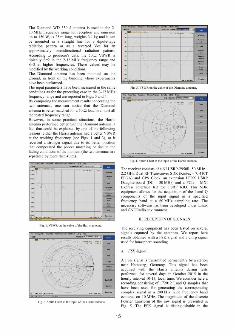
The Diamond WD 330 J antenna is used in the 2-

30 MHz frequency range for reception and emission

up to 150 W, is 25 m long, weights 3.1 kg and it can

be mounted in a straight line for a dipole-type

radiation pattern or as a reversed Vee for an

approximately omnidirectional radiation pattern.

According to producer's data, the 50 VSWR is

tipically S=2 in the 2-18 MHz frequency range and

S=3 at higher frequencies. These values may be

modified by the working conditions.

The Diamond antenna has been mounted on the

ground, in front of the building where experiments

have been performed.

The input parameters have been measured in the same

conditions as for the preceding case in the 3-12 MHz

frequency range and are reported in Figs. 3 and 4.

By comparing the measurement results concerning the

two antennas, one can notice that the Diamond

antenna is better matched for a 50 load in almost all

the tested frequency range.

However, in some practical situations, the Harris

antenna performed better than the Diamond antenna, a

fact that could be explained by one of the following

reasons: either the Harris antenna had a better VSWR

at the working frequency (see Figs. 1 and 3), or it

received a stronger signal due to its better position

that compesated the poorer matching or due to the

fading conditions of the moment (the two antennas are

separated by more than 40 m).

The receiver consists of a NI USRP-2950R, 50 MHz –

2.2 GHz Dual RF Transceiver SDR (Kintex – 7, 410T

FPGA) and GPS Clock, an extension LFRX USRP

Daughterboard (DC – 30 MHz) and a PCIe – MXI

Express Interface Kit for USRP RIO. This SDR

equipment allows for the acquisition of the I and Q

components of the input signal in a specified

frequency band at a 60 MHz sampling rate. The

necessary software has been developed under Linux

and GNURadio environment.

III RECEPTION OF SIGNALS

The receiving equipment has been tested on several

signals captured by the antennas. We report here

results obtained with a FSK signal and a chirp signal

used for ionosphere sounding.

A. FSK Signal

A FSK signal is transmitted permanently by a station

near Hamburg, Germany. This signal has been

acquired with the Harris antenna during tests

performed for several days in October 2015 in the

hourly interval 10-13, local time. We consider here a

recording consisting of 172012 I and Q samples that

have been used for generating the corresponding

complex signal in a 200 kHz wide frequency band

centered on 10 MHz. The magnitude of the discrete

Fourier transform of the raw signal is presented in

Fig. 5. The FSK signal is distinguishable in the

Fig. 3. VSWR on the cable of the Diamond antenna.

Fig. 4. Smith Chart at the input of the Harris antenna.

Fig. 1. VSWR on the cable of the Harris antenna.

Fig. 2. Smith Chart at the input of the Harris antenna.

15

vicinity of the center frequency (10 MHz). Other HF

signals are present in the received spectrum. For a

clearer rendering of the signals, allowing for a more

precise frequency assessment, the following

processing has been performed on the raw signal: a

1024 – sample wide Hamming window has been

displaced along the signal with a step of 500 samples.

The Discrete Fourier Transform has been performed

at each step and the results have been averaged. The

magnitude of the result is displayed in Fig. 6.

The two maxima of the FSK signal are now clearly

visible at 9.99 MHz and 10.02 MHz respectively.

Other signals are present at 9.365, 9.766, 9.955,

10.17, 10.31, 10.68, 10.73 and 10.86 MHz. Averaging is not a good option if (in)stability in time

determined by the variation in electron density of the

ionosphere, fading and the Doppler shift caused by

displacement of layers have to be investigated.

Therefore, a time-frequency analysis of the signal has

been performed, and reported in Fig. 7. A 1024 –

sample rectangular window and a 32 – sample step

have been used for the representation. The experiment

demonstrates the variability of reception in the HF

range, clearly visible on the 10.86 MHz signal in Fig.

7, but also visible on the FSK signal.

B. Chirp Signal

A modern solution to obtain real-time information

about the ionosphere is the ionosonde, a special type

of radar system, consisting of a transmitter equipment

that sweeps all or part of the HF frequency range, and

it transmits short pulses or continuous signals. These

signals, reflected at various layers of the ionosphere,

are collected by the receiver and analysed by an

appropriate control system.

Ionospheric sounding can be vertically or oblique.

Vertical sounders transmit the wave vertically and the

reflected wave is received by the receiver placed in

the vicinity of the transmitter. Oblique ionospheric

sounding allows for monitoring the radio channel over

large and very large distances, impossible to achieve

by other techniques. This technique also allows a

single receiver to receive signals from several

transmitters located in different geographical places.

In both cases, the signal round trip delay allows to

calculate the height at which the reflection occurs and

to estimate the critical frequency and the

communication distance for a given frequency.

In this paper we focus only on the particular

ionosonde type sounder known as the Chirp Sounder,

that transmits a low power Frequency Modulated

Continuous Wave (FMCW) or chirp, i.e. a continuous

signal in which the instantaneous frequency increases

linearly with time. Chirp sounders usually transmit in

range 2 – 30 MHz and some of the sounders skip

some particular frequencies used for critical

communications.

Software defined radio is a very powerful and

versatile tool that can be used both for generating and

receiving the chirp sounding signal [12]. In our

experiments we have used the USRP 2950R based

receiving system and the two antennas described

above.

There are many ionosondes that transmit chirp signals

but the information about their location and time

parameters are either incomplete or difficult to find.

The transmitting stations are hard to identify as chirp

signal does not contain any information in addition to

the FM-CW wave.

For testing our receiving system, we have found a

reliable chirp sounder located near Akrotini, Cyprus,

approximately 1600 km from reception point.

Fig. 7. Time-frequency representation of the received signal.

Fig. 6. Averaged spectrum of the received signal.

Fig. 5. Spectrum of the received signal.

16

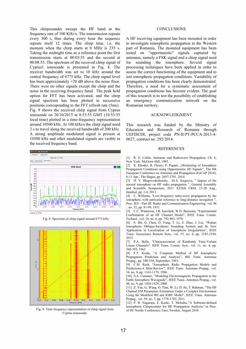
This chirpsounder sweeps the HF band at the

frequency rate of 100 KHz/s. The transmission repeats

every 300 s, thus during every hour the sequence

repeats itself 12 times. The chirp time, i.e. the

moment when the chirp starts at 0 MHz is 235 s.

Taking the midnight time as a reference point the first

transmission starts at 00:03:55 and the second at

00:08:55. The spectrum of the received chirp signal of

Cyprus1 ionosonde is presented in Fig. 8. The

receiver bandwidth was set to 10 kHz around the

central frequency of 6775 kHz. The chirp signal level

has been approximately +20 dB above the noise floor.

There were no other signals except the chirp and the

noise in the receiving frequency band. The peak hold

option for FFT has been activated, and the chirp

signal spectrum has been plotted in successive

positions corresponding to the FFT refresh rate (5ms).

Fig. 9 shows the received chirp signal from Cyprus

ionosonde on 20/10/2015 at 8:53:55 GMT (10:53:55

local time) plotted in a time-frequency representation

around 10500 kHz. At 100 kHz/s the chirp signal need

2 s to travel along the received bandwidth of 200 kHz.

A strong amplitude modulated signal is present at

10500 kHz and other modulated signals are visible in

the received frequency band.

Fig. 9. Time-frequency representation of chirp signal from

Cyprus ionosonde.

CONCLUSIONS

A HF receiving equipment has been mounted in order

to investigate ionospheric propagation in the Western

part of Romania. The mounted equipment has been

tested on "opportunistic" signals captured by

antennas, namely a FSK signal and a chirp signal used

for sounding the ionosphere. Several signal

processing techniques have been applied in order to

assess the correct functioning of the equipment and to

test ionospheric propagation conditions. Variability of

propagation conditions has been clearly demonstrated.

Therefore, a need for a systematic assessment of

propagation conditions has become evident. The goal

of this research is to test the possibility of establishing

an emergency communication network on the

Romanian territory.

ACKNOWLEDGMENT

This research was funded by the Ministry of

Education and Research of Romania through

UEFISCDI, project code PN-II-PT-PCCA-2013-4-

0627, contract no. 292/2014.

REFERENCES

[1] R. E. Collin, Antennas and Radiowave Propagation, Ch. 6,

New York: McGraw-Hill, 1985.

[2] K. Khoder, R. Fleury, P. Pagani, „Monitoring of Ionosphere

Propagation Conditions using Opportunistic HF Signals”, The 8th

European Conference on Antennas and Propagation (EuCAP 2014),

6-11 Apr., The Hague, pp. 2697-2701, 2014.

[3] D. V. Blagoveshchensky, M.A. Sergeeva, " Impact of the

auroral ionosphere on HF radio propagation ", General Assembly

and Scientific Symposium, 2011 XXXth URSI, 13-20 Aug.,

Istanbul, pp. 1-4, 2011.

[4] C. Williams, "Low-frequency radio-wave propagation by the

ionosphere, with particular reference to long-distance navigation ",

Proc. IEE - Part III: Radio and Communication Engineering vol. 98

, no. 52, pp. 81-99, 1951.

[5] C.C. Watterson, J.R. Juroshek, W.D. Bensema, "Experimental

Confirmation of an HF Channel Model", IEEE Trans. Comm.

Technol., vol. 18, no. 6, pp. 792-803, 1970.

[6] S. Shi, G. Chen, G. Yang, T. Li, Z. Zhao, J. Liu, “Wuhan

Ionospheric Oblique-Incidence Sounding System and Its New

Application in Localization of Ionospheric Irregularities”, IEEE

Trans. Geoscience Remote Sens., vol. 53, no. 4, pp. 2185-2194,

2015.

[7] P.A. Bello, "Characterization of Randomly Time-Variant

Linear Channels", IEEE Trans. Comm. Syst., vol. 11, no. 4, pp.

360-393, 1963.

[8] F.T. Koide, “A Computer Method of HF Ionospheric

Propagation Prediction and Analysis”, IRE Trans. Antennas

Propag., pp. 540-558, September, 1963.

[9] C.M. Rush, “Ionospheric Radio Propagation Models and

Predictions-A Mini-Review”, IEEE Trans. Antennas Propag., vol.

34. no. 9, pp. 1163-1170, 1986.

[10] S.A. Cummer, “Modeling Electromagnetic Propagation in the

Earth–Ionosphere Waveguide”, IEEE Trans. Antennas Propag., vol.

48, no. 9, pp. 1420-1429, 2000.

[11] Z. Yan, G. Wang, G. Tian, W. Li, D. Su, T. Rahman, “The HF

Channel EM Parameters Estimation Under a Complex Environment

Using the Modified IRI and IGRF Model”, IEEE Trans. Antennas

Propag., vol. 59, no. 5, pp. 1778-1783, 2011.

[12] P. B. Nagaraju, E. Koski, T. Melodia, "A Software-defined

Ionospheric Chirpsounder for HF Propagation Analysis," in Proc.

of HF Nordic Conference, Faro, Sweden, August 2010.

Fig. 8. Spectrum of chirp signal around 6775 kHz.

17

Buletinul Ştiinţific al Universităţii Politehnica Timişoara


Volume 60(74), Issue 2, 2015

Cluster Capacity Increase through eICIC Technology - An

Experimental Analysis

Ionel Petruţ1 Marius Oteşteanu

2 Cornel Balint

2 Georgeta Budura

2

1 Faculty of Electronics and Telecommunications, Communications Dept., Alcatel-Lucent Timisoara, Romania

Bd. V. Parvan 2, 300223 Timisoara, Romania, [email protected] 2 Faculty of Electronics and Telecommunications, Communications Dept.

Bd. V. Parvan 2, 300223 Timisoara, Romania, marius.otesteanu; cornel.balint; [email protected]

Abstract–In order to have a successful transition from a

legacy network architecture with only a macro layer

towards heterogeneous networks (HetNet) consisting of

different base stations types, diverse technical solutions

and innovations are enabled. In this article we perform a

set of experiments in a real LTE HetNet cabled network

that implements time-domain enhanced Inter-Cell

Interference Coordination (eICIC) concept. Analyzing

the network behavior the benefits and characteristics of

this solution are outlined and explained. We

experimentally determine the optimal value for eICIC

offset parameter and the minimum number of small cells

for a cluster with increased capacity through eICIC

activation.

Keywords: HetNet, eICIC, Cell Range Expansion,

Almost Blank Subframes.

I. INTRODUCTION

The increased demand for mobile broadband services

with higher data rates recently became a challenge for

the mobile telecommunications networks. Since the

radio spectral efficiency approaches its fundamental

limits, further improvements are possible only by new

network techniques. The widely adopted solution for

increasing network capacity is network densification

using small cells. However the gain obtained by rising

the node deployment density is significantly reduced,

due to severe inter-cells interferences. In LTE Rel-8,

Inter-Cell Interference Coordination (ICIC) is

performed over the frequency domain by messages

transmitted across a standardized interface X2 that

allows adaptive fractional frequency reuse [1, 2].

A solution to these problems is offered by the

introduction of heterogeneous architecture in the

LTE-Advanced standardization [3, 4]. The resulted

solution, HetNet, consists of a mix of Macrocells

(MC) equipped with high-power nodes, and small

cells (SC) equipped with low-power eNodeB (eNB),

in order to enhanced the overall system capacity and

to efficiently accommodate high traffic volume in

small local areas [3, 4, 5].

The new architecture also shows some impairments:

The high level of interferences at the edge of SC;

Inefficient resources utilization inside SC due to

the reduced number of User Equipment (UE)

connected to SC compared to MC.

In LTE Rel-10, 3GPP introduces two approaches to

coordinate inter-layer interferences in HetNet

deployment scenarios.

In one approach, interferences avoidance is addressed

by means of ICIC in frequency domain, relying on

carrier-aggregation (CA) [1].

In the other approach, interferences avoidance and

inefficient resources utilization inside SC are

addressed by means of ICIC in time domain. The

eICIC new technique overcomes these two problems

by extending the SC radius by adding the so called

Cell Range Expansion (CRE) and by reserving for this

area a part of MC resources through Almost Blank

SubFrames (ABS) approach [5, 6, 7, 8, 9].

The rest of our paper is organized as follows: Section

II is dedicated to eICIC technique in LTE and reveals

theoretical aspects of CRE. In Section III on the basis

of experimental analysis we determine an optimal

value of the CRE parameter that maximizes the global

throughput of a HetNet cluster consisting of a MC and

a single SC. The results are extended for a cluster that

includes several SC, concluding that HetNet benefits

exist for a minimum number of SC in the cluster.

II. eICIC IN LTE

The eICIC concept was developed in order to reduce

the interferences in HetNet clusters operating with

reuse factor 1. The cluster assures LTE services for a

specific geographical area and consists of one Macro

cell and several small cells. These small cells are used

for densification and capacity increase.

There are two mechanisms that are activated in the

network when the eICIC is implemented.

On the small cells side the cell coverage is extended

using CRE in order to allow macro layer decongestion

and more efficient resources utilization in SC. The

extension is made by adding a handover offset

parameter ”OCRE” to the SC reference signal received

power (RSRP) that triggers handover for UE located

18

nearby SC edge area preferentially toward the SC

even when it is not the strongest cell.

Although CRE enables higher user offloading from

MC on to SC, the UE connected to SC with large

CRE offset can suffer severe interferences from the

MC. In the CRE area the received signal power from

MC is higher than the received signal from SC.

On the Macro cell side the resources allocation

algorithm is modified in order to reserve a percentage

of the radio resources for SC. This resources

reservation is called ABS and according to standard

can be between 0-70% from total amount of MS radio

resources. In this way MC creates protected

subframes for SC by turning off its downlink

transmission (or just reducing the power of some

downlink signals) in certain subframes. The

informations regarding ABS subframes are known a

priori at all SC in the cluster via X2 interface.

Consequently, these resources can be used by all

small cells inside the cluster, in order to avoid the

interferences and to extend the initial coverage area

for each small cell. During ABS subframes, the MC

does not transmit UE data (Physical Dedicated

Control/Data Channels PDCCH/PDSCH) but may

transmit cell reference signals (CRS), control

channels, as well as broadcast and paging information

in order to ensures legacy UE support.

In Fig. 1 we show a typical HetNet cluster in a dense

urban area. Before eICIC activation, the users from

the dotted area are served by Macro cell and they have

poor signal quality due to high level of interferences.

After eICIC activation the small cells radius is

proportionally increased with the offset parameter,

drown in Fig. 1 as dotted rings.

Small cells eNB will allocate reserved resources for

users located in dotted zones. The same resources will

be reused by every small cell in the cluster; as

consequence the overall end user throughput per

cluster is increased proportionally with the number of

small cells in the cluster.

The small cell limit corresponds to the handover

trigger point, where is satisfied the handover

condition expressed as follows:

MC SC CRER R HOM O (1)

where MCR and SCR are the RSRP value for macro and

small cell respectively, HOM is the handover margin

and CREO is the offset that determine the CRE area.

Fig. 1. HetNet cluster using CRE.

Fig. 2 shows the received power from small cell and

macro cell and the CRE area for a given offset

according to (1).

The benefits of eICIC feature can be summarized as

follows:

Increase the spectral efficiency by reducing the

level of interferences in the most affected areas

(at the border of small cells). This gain is evident

even when the cluster consists of a single small

cell;

Increase the overall cluster throughput. This

increase is mostly visible in networks consisting

of a reduced number of small cells.

III. EXPERIMENTAL ANALYSIS AND RESULTS

The experiments are conducted on a 2.6 GHz test

branch in a cabled environment using a basic cluster.

The cluster consists of two eNB: one macro cell and

one small cell eNB that emit both in 20MHz

bandwidth. The UE is connected using a channel

emulator, that simulates a real channel with noise and

fading.

Programmable attenuation equipment simulates the

UE movement with 5km/h constant speed,

corresponding to a pedestrian channel [10]. Inside the

cluster an user equipment (CAT4 UE) is able to use

all available resources allocated by eNB.

The aim of the experiments is to analyze the eICIC

functionality in specific network architecture. In all

the experimental scenarios we consider the same 30%

ratio for ABS resources reservation and different

range expansion offset values.

In the experiments initially the UE is attached to the

small cell and has ongoing DL transfer, reaching the

maximum cell capacity of about 100 Mbps. From this

point UE starts moving with constant speed towards

the Macro cell. The UE performs HO and changes the

serving cell to macro cell, continuing to move inside

Macro area until reaching the best signal quality.

After that the UE returns back to the small cell

through HO moving with the same speed until he

reaches again the best signal quality also on small

cell.

For each experiment we report averaged values

computed based on 300 iterations.

The first scenario for eICIC analysis corresponds to

the simplest case when we have only one small cell in

the cluster, that uses in CRE area the resources

reserved by macro cell.

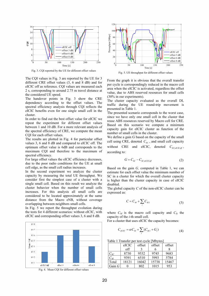
In the first experiment we measure and plot in Fig. 3

the Channel Quality Indicator (CQI).

Fig. 2. Small cell offset and CRE.

Small

Cell

Cell

Expansion

Range

Macro

Cell

Small cell

RSRP Macro cell

RSRP

CRE

Offset

Small cell

Small cell radius

Macro cell

Distance

RM

C,

RS

C

19

0 50 100 150 200 2504

6

8

10

12

14

16

Time [s]

CQ

I

eICIC off

offset 3 dB

offset 6 dB

offset 8 dB

Fig. 3. CQI reported by the UE for different offset values

The CQI values in Fig. 3 are reported by the UE for 3

different CRE offset values (3, 6 and 8 dB) and for

eICIC off as reference. CQI values are measured each

2 s, corresponding to around 2.75 m travel distance at

the considered UE speed.

The handover points in Fig. 3 show the CRE

dependency according to the offset values. The

spectral efficiency analysis through CQI reflects the

eICIC benefits even for one single small cell in the

cluster.

In order to find out the best offset value for eICIC we

repeat the experiment for different offset values

between 1 and 10 dB. For a more relevant analysis of

the spectral efficiency of CRE, we compute the mean

CQI for each offset values.

The results are plotted in Fig. 4 for particular offset

values 3, 6 and 8 dB and compared to eICIC off. The

optimum offset value is 6dB and corresponds to the

maximum CQI and therefore to the maximum of

spectral efficiency.

For large offset values the eICIC efficiency decreases,

due to the poor radio conditions for the UE at small

cell edge, as the small cell radius increases.

In the second experiment we analyze the cluster

capacity by measuring the total UE throughput. We

consider first the simplest case of a cluster with a

single small cell. Based on this result we analyze the

cluster behavior when the number of small cells

increases. For this analysis all small cells are

considered to be located approximately at the same

distance from the Macro eNB, without coverage

overlapping between neighbors small cells.

In Fig. 5 we report the throughput evolution during

the tests for 4 different scenarios: without eICIC, with

eICIC and corresponding offset values 3, 6 and 8 dB.

Fig. 4. Mean CQI for different offset values

0 50 100 150 200 2500

20

40

60

80

100

120

Time [s]

Th

rou

gh

pu

t [M

bp

s]

eICIC off

offset 3 dB

offset 6 dB

offset 8 dB

Fig. 5. UE throughput for different offset values

From the graph it is obvious that the overall transfer

per cycle is correspondingly reduced in the macro cell

area when the eICIC is activated, regardless the offset

value, due to ABS reserved resources for small cells

(30% in our experiments).

The cluster capacity evaluated as the overall DL

traffic during the UE round-trip movement is

presented in Table 1.

The presented scenario corresponds to the worst case,

since we have only one small cell in the cluster that

reuse ABS resources reserved by Macro cell for CRE.

Based on this scenario we compute a minimum

capacity gain for eICIC cluster as function of the

number of small cells in the cluster.

We define a gain G based on the capacity of the small

cell using CRE, denoted SCC , and small cell capacity

without CRE and eICIC, denoted |SC eICICoffC ,

according to:

|SC SC eICICoffG C C (2)

Based on the gain G, computed in Table 1, we can

estimate for each offset value the minimum number of

SC in a cluster for which the overall cluster capacity

is higher than the cluster capacity in case of eICIC

disabled.

The global capacity C of the non-eICIC cluster can be

expressed as:

M SCi

i

C C C (3)

where CM is the macro cell capacity and CSi the

capacity of the i-th small cell.

For a cluster that uses eICIC the capacity becomes:

( )eICIC M SCi i

i

C C C G (4)

Table 1 Transfer per test cycle [Mbytes]

eICIC

off

offset

3

offset

6

offset

8

CSC 8730 9532 9745 9683

CM 9391 6510 5993 5784

Total 18121 16042 15738 15467

Gain G 0 802 1015 953

20

where is the ratio of the macro cell resources

reserved for ABS, and iG is the gain of the i-th small

cell.

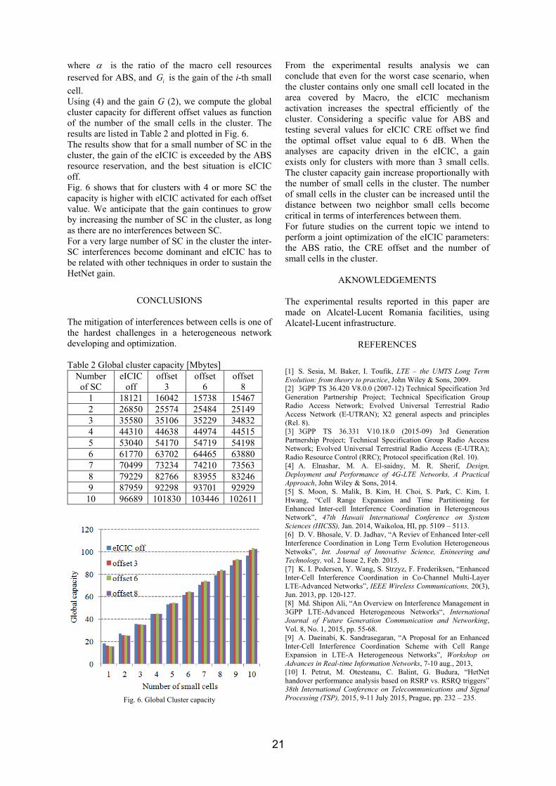
Using (4) and the gain G (2), we compute the global

cluster capacity for different offset values as function

of the number of the small cells in the cluster. The

results are listed in Table 2 and plotted in Fig. 6.

The results show that for a small number of SC in the

cluster, the gain of the eICIC is exceeded by the ABS

resource reservation, and the best situation is eICIC

off.

Fig. 6 shows that for clusters with 4 or more SC the

capacity is higher with eICIC activated for each offset

value. We anticipate that the gain continues to grow

by increasing the number of SC in the cluster, as long

as there are no interferences between SC.

For a very large number of SC in the cluster the inter-

SC interferences become dominant and eICIC has to

be related with other techniques in order to sustain the

HetNet gain.

CONCLUSIONS

The mitigation of interferences between cells is one of

the hardest challenges in a heterogeneous network

developing and optimization.

Table 2 Global cluster capacity [Mbytes]

Number

of SC

eICIC

off

offset

3

offset

6

offset

8

1 18121 16042 15738 15467

2 26850 25574 25484 25149

3 35580 35106 35229 34832

4 44310 44638 44974 44515

5 53040 54170 54719 54198

6 61770 63702 64465 63880

7 70499 73234 74210 73563

8 79229 82766 83955 83246

9 87959 92298 93701 92929

10 96689 101830 103446 102611

Fig. 6. Global Cluster capacity

From the experimental results analysis we can

conclude that even for the worst case scenario, when

the cluster contains only one small cell located in the

area covered by Macro, the eICIC mechanism

activation increases the spectral efficiently of the

cluster. Considering a specific value for ABS and

testing several values for eICIC CRE offset we find

the optimal offset value equal to 6 dB. When the

analyses are capacity driven in the eICIC, a gain

exists only for clusters with more than 3 small cells.

The cluster capacity gain increase proportionally with

the number of small cells in the cluster. The number

of small cells in the cluster can be increased until the

distance between two neighbor small cells become

critical in terms of interferences between them.

For future studies on the current topic we intend to

perform a joint optimization of the eICIC parameters:

the ABS ratio, the CRE offset and the number of

small cells in the cluster.

AKNOWLEDGEMENTS

The experimental results reported in this paper are

made on Alcatel-Lucent Romania facilities, using

Alcatel-Lucent infrastructure.

REFERENCES

[1] S. Sesia, M. Baker, I. Toufik, LTE – the UMTS Long Term

Evolution: from theory to practice, John Wiley & Sons, 2009.

[2] 3GPP TS 36.420 V8.0.0 (2007-12) Technical Specification 3rd

Generation Partnership Project; Technical Specification Group

Radio Access Network; Evolved Universal Terrestrial Radio

Access Network (E-UTRAN); X2 general aspects and principles

(Rel. 8).

[3] 3GPP TS 36.331 V10.18.0 (2015-09) 3rd Generation

Partnership Project; Technical Specification Group Radio Access

Network; Evolved Universal Terrestrial Radio Access (E-UTRA);

Radio Resource Control (RRC); Protocol specification (Rel. 10).

[4] A. Elnashar, M. A. El-saidny, M. R. Sherif, Design,

Deployment and Performance of 4G-LTE Networks, A Practical

Approach, John Wiley & Sons, 2014.

[5] S. Moon, S. Malik, B. Kim, H. Choi, S. Park, C. Kim, I.

Hwang, “Cell Range Expansion and Time Partitioning for

Enhanced Inter-cell Interference Coordination in Heterogeneous

Network”, 47th Hawaii International Conference on System

Sciences (HICSS), Jan. 2014, Waikoloa, HI, pp. 5109 – 5113.

[6] D. V. Bhosale, V. D. Jadhav, “A Reviev of Enhanced Inter-cell

Interference Coordination in Long Term Evolution Heterogeneous

Netwoks”, Int. Journal of Innovative Science, Enineering and

Technology, vol. 2 Issue 2, Feb. 2015.

[7] K. I. Pedersen, Y. Wang, S. Strzyz, F. Frederiksen, “Enhanced

Inter-Cell Interference Coordination in Co-Channel Multi-Layer

LTE-Advanced Networks”, IEEE Wireless Communications, 20(3),

Jun. 2013, pp. 120-127.

[8] Md. Shipon Ali, “An Overview on Interference Management in

3GPP LTE-Advanced Heterogeneous Networks“, International

Journal of Future Generation Communication and Networking,

Vol. 8, No. 1, 2015, pp. 55-68.

[9] A. Daeinabi, K. Sandrasegaran, “A Proposal for an Enhanced

Inter-Cell Interference Coordination Scheme with Cell Range

Expansion in LTE-A Heterogeneous Networks”, Workshop on

Advances in Real-time Information Networks, 7-10 aug., 2013,

[10] I. Petrut, M. Otesteanu, C. Balint, G. Budura, “HetNet

handover performance analysis based on RSRP vs. RSRQ triggers”

38th International Conference on Telecommunications and Signal

Processing (TSP), 2015, 9-11 July 2015, Prague, pp. 232 – 235.

21



Volume 60(74), Issue 2, 2015

Review over different diagnostic specifications and testing tools used in automotive domain

Bianca Enache1 Marius Otesteanu2 Daniel Tiuc3

1 Faculty of Electronics and Telecommunications, Communications Dept. Bd. V. Parvan 2, 300223 Timisoara, Romania, e-mail [email protected] 2 Faculty of Electronics and Telecommunications, Communications Dept. Bd. V. Parvan 2, 300223 Timisoara, Romania, e-mail [email protected] 3 Faculty of Mechanics, Industrial Dept. Bd. V. Parvan 2, 300223 Timisoara, Romania, e-mail [email protected]

Abstract – This paper presents a review over the most popular tools used in automotive industry for black-box testing process. It presents the benefits of diagnostic specifications and diagnostic testers. It also reflects how important is to have a template that can satisfy any diagnostic data. Index Terms—testing, tools, automotive, diagnostics, requirements.

I. INTRODUCTION

The vehicle functionality is in continuing research. The entire system functionality is tested using black-box testing. This testing type verifies the system behavior using an input-actions-output model. It is seen as an opaque system, without any interest about the interior. It is checked that for a set of inputs, applying a set of actions, is obtained a set of outputs according to the requirements. Some of the tools that are used in automotive domain at system test level for diagnostic are[3]: CANdelaStudio, ODXStudio, CANoe.Diva, Indigo, CANoe, CANape, vFlash. The CANdelaStudio is used to specify the diagnostic features of an ECU, while the ODXStudio is used for ant ODX category of ASAM ODX 2.0.1. or ISO ODX 2.2. For an automated environment the ECU diagnostic software validations is performed using CANoe.DiVa, CANoe, Indigo and CANape. Here the Electronic Control Unit (ECU) test cases are generated and the execution process is automated entirely or half. The vFlash tool is very efficient and user friendly to flash over Controller Area Network (CAN), Local Interconnect Network (LIN) or Ethernet.

II. THE DIAGNOSTIC TOOLS OVERVIEW

In this chapter each tool will be treated separately. It will be proved the impact of it in the daily job of a system test engineer.

The first one, CANoe.Diagonostic Integration and Validation Assistant(CANoe.DiVa) represents one of the ways for obtaining automated and data based generation of test cases that can be reproduced. It can be considered the link between CANdela and CANoe. It generates some automated ECU specific test module for CANoe using diagnostic requirements. From standards point of view this tool supports[5]: ISO 14229 Unified Diagnostic Services (UDS): 2006/2013, ISO 15765 Diagnostics on CAN, ISO15031/J1979 On Board Diagnostics, etc. Another feature of CANoe.Diva is represented by the modality of mapping the customer or system requirements to test cases results. Using DOORS for storage the customer requirements for instance the CANdelaStudio tool can facilitate the import and export process. It is able to generate requirements from diagnostic information and diagnostic information from requirements. In order to access the vehicle system through UMTS/GPRS the Indigo tool can be used. It will be discussed in the next chapter. The vFlash tool is coming with the possibility to flash in parallel 8 ECUs.

III. DIAGNOSTIC CONCEPT USING REQUIREMENTS

Each customer is unique and in order to cover all the needs the diagnostic information is combined in such a manner to be customized easily[1].

Fig. 1. The diagnostic data template

22

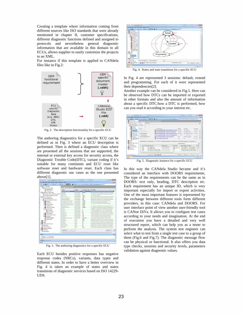
Creating a template where information coming from different sources like ISO standards that were already mentioned in chapter II, customer specifications, different diagnostic functions defined and assigned to protocols and nevertheless general diagnostic information that are available in this domain to all ECUs, allows supplier to easily customize the projects to an XML. For instance if this template is applied to CANdela files like in Fig.2:

Fig. 2. The description functionality for a specific ECU

The authoring diagnostics for a specific ECU can be defined as in Fig. 3 where an ECU description is performed. Then is defined a diagnostic class where are presented all the sessions that are supported, the internal or external key access for security access, the Diagnostic Trouble Code(DTC), variant coding if it’s suitable for many continents and ECU reset like software reset and hardware reset. Each class has different diagnostic use cases as the one presented above[1].

Fig. 3. The authoring diagnostics for a specific ECU

Each ECU besides positive responses has negative response codes (NRCs), variants, data types and different states. In order to have a better overview in Fig. 4 is taken an example of states and states transitions of diagnostic services based on ISO 14229-UDS.

Fig. 4. States and state transitions for a specific ECU

In Fig. 4 are represented 3 sessions: default, extend and programming. For each of it were represented their dependencies[2]. Another example can be considered in Fig.5. Here can be observed how DTCs can be imported or exported in other formats and also the amount of information about a specific DTC:how a DTC is performed, how can you read it according to your interest etc.

Fig. 5. Diagnostic instance for a specific ECU

In this way the CANdela Studio became and it’s considered an interface with DOORS requirements. The type of the requirements can be the same as in DOORS: text only, heading, DTC description etc. Each requirement has an unique ID, which is very important especially for import or export activities. One of the most important features is represented by the exchange between different tools form different providers, in this case: CANdela and DOORS. For user interface point of view another user-friendly tool is CANoe DiVa. It allows you to configure test cases according to your needs and imagination. At the end of execution you have a detailed and very well structured report, which can help you as a tester to perform the analysis. The system test engineer can select what to test from a single test case to a group of them (Fig.6 and Fig.7). The diagnostic message flow can be physical or functional. It also offers you data type checks, sessions and security levels, parameters validation against diagnostic values.

23

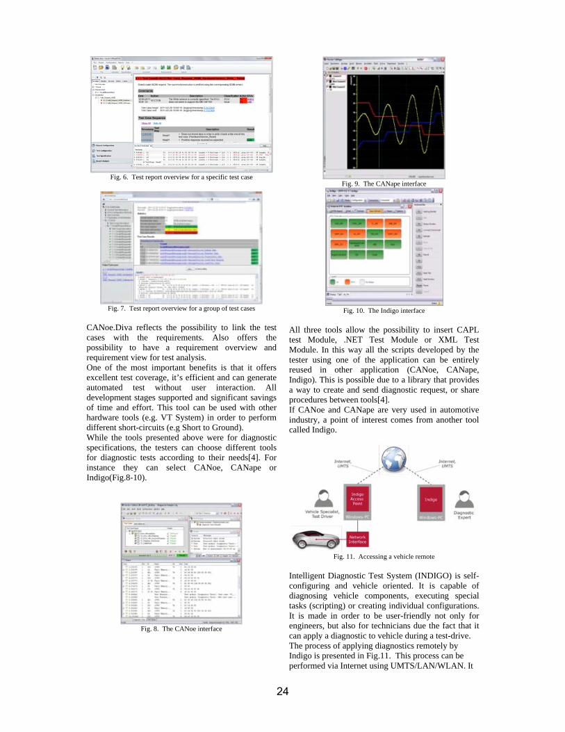
Fig. 6. Test report overview for a specific test case

Fig. 7. Test report overview for a group of test cases

CANoe.Diva reflects the possibility to link the test cases with the requirements. Also offers the possibility to have a requirement overview and requirement view for test analysis. One of the most important benefits is that it offers excellent test coverage, it’s efficient and can generate automated test without user interaction. All development stages supported and significant savings of time and effort. This tool can be used with other hardware tools (e.g. VT System) in order to perform different short-circuits (e.g Short to Ground). While the tools presented above were for diagnostic specifications, the testers can choose different tools for diagnostic tests according to their needs[4]. For instance they can select CANoe, CANape or Indigo(Fig.8-10).

Fig. 8. The CANoe interface

Fig. 9. The CANape interface

Fig. 10. The Indigo interface

All three tools allow the possibility to insert CAPL test Module, .NET Test Module or XML Test Module. In this way all the scripts developed by the tester using one of the application can be entirely reused in other application (CANoe, CANape, Indigo). This is possible due to a library that provides a way to create and send diagnostic request, or share procedures between tools[4]. If CANoe and CANape are very used in automotive industry, a point of interest comes from another tool called Indigo.

Fig. 11. Accessing a vehicle remote

Intelligent Diagnostic Test System (INDIGO) is self-configuring and vehicle oriented. It is capable of diagnosing vehicle components, executing special tasks (scripting) or creating individual configurations. It is made in order to be user-friendly not only for engineers, but also for technicians due the fact that it can apply a diagnostic to vehicle during a test-drive. The process of applying diagnostics remotely by Indigo is presented in Fig.11. This process can be performed via Internet using UMTS/LAN/WLAN. It

24

assumes to work for low data traffic and high security. The remote access can be done using a Windows tablets[4].

IV. CONCLUSIONS The tools that were presented are user-friendly not only from engineers point of view, but also from customers and are very popular in automotive industry nowadays. All are based on multi-brand solution, by using one architecture for many other brands. The testers can configure as much as they wish and can be linked between them.

ACKNOWLEDGMENT This paper is supported by the Sectoral Operational Programme Human Resources Development

POSDRU/159/1.5/S/137516 financed from the European Social Fund and by the Romanian Government. This work was partially supported by the strategic grant POSDRU/159/1.5/S/134378 (2014) of the Ministry of National Education, Romania, co-financed by the European Social Fund – Investing in People, within the Sectoral Operational Programme Human Resources Development 2007-2013.

REFERENCES [1] http://vector.com/vi_diagnostics_en.htmlaccessed :23.08.2015 [2] http://vector.com/vi_training_en.html accessed : 24.08.2015 [3] http://vector.com/vi_portfolio_en.html accessed: 25.08.2015 [4] http://vector.com/vi_diag_tester_en.htmlaccessed:24.08.2015 [5] Verband der Automobilindustrie, Quality management in the Automotive Industry Quality Assurance of Supplies, VDA and QMC,2004.

25



Volume 61(75), Issue 1, 2016

Instructions for authors at the Scientific Bulletin of the Politehnica University of Timisoara - Transactions on

Electronics and Communications

First Author1 Second Author2

1 Faculty of Electronics and Telecommunications, Communications Dept. Bd. V. Parvan 2, 300223 Timisoara, Romania, e-mail [email protected] 2 Faculty of Electronics and Telecommunications, Communications Dept. Bd. V. Parvan 2, 300223 Timisoara, Romania, e-mail [email protected]

Abstract – These instructions present a model for editing the papers accepted at the Scientific Bulletin of “Politehnica” University of Timisoara, Transactions on Electronics and Communications. The abstract should contain the description of the problem, methods, solutions and results in a maximum of 12 lines. No references are allowed here. Keywords: editing, Bulletin, author

I. INTRODUCTION

The page format is A4. The articles must be of 6 pages or less, tables and figures included.

II. GUIDELINES

The paper should be sent in this standard form. Use a good quality printer, and print on a single face of the sheet. Use a double column format with 0.5 cm in between columns, on an A4, portrait oriented, standard size. The top and bottom margins should be of 2.28 cm, and the left and right margins of 2.54 cm. Microsoft Word™ for Windows is recommended as a text editor. Choose Times New Roman fonts, and single spaced lines. Font sizes should be: 18 pt bold for the paper title, 12 pt for the author(s), 9 pt bold for the abstract and keywords, 10 pt capitals for the section titles, 10 pt italic for the subsection titles; distance between section numbers and titles should be of 0.25 cm; use 10 pt for the normal text, 8 pt for affiliation, footnotes, figure captions, and references.

III. FIGURES AND TABLES Figures should be centered, and tables should be left aligned, and should be placed after the first reference in the text. Use abbreviations such as “Fig.1.” even at the beginning of the sentence. Leave an empty line before and after equations. Equation numbering should be simple: (1), (2), (3) … and right aligned:

∫− −=a

adtytx ττ )()( . (1)

IV. ABOUT REFERENCES References should be numbered in a simple form [1], [2], [3]…, and quoted accordingly [1]. References are not allowed in footnotes. It is recommended to mention all authors; “et al.” should be used only for more than 6 authors. Table 1

Parameter Value Unit I 2.4 A U 10.0 V

V. REMARKS A. Abbreviations and acronyms Abbreviations and acronyms should be explained when they appear for the first time in the text. Abbreviations such as IEEE, IEE, SI, MKS, CGS, ac, dc and rms need no further explanation. It is recommended not to use abbreviations in section or subsection titles.

Fig. 1. Amplitudes in the standing wave

26

B. Further recommendations The International System of units is recommended. Do not mix SI and CGS. Preliminary, experimental results are not accepted. Roman section numbering is optional.

REFERENCES [1] A. Ignea, “Preparation of papers for the International Symposium Etc. ’98”, Buletinul Universităţii “Politehnica”, Seria Electrotehnica, Electronica si Telecomunicatii, Tom 43 (57), 1998, Fascicola 1, 1998, pp. 81. [2] R. E. Collin, Foundations for Microwave Engineering, Second Edition, McGraw-Hill, Inc., 1992. [3] http://www.tc.etc.upt.ro/bulletin

27

Buletinul ştiinţific al Universităţii Politehnica din ... · Buletinul ştiinţific al...

Documents

Transcript of Buletinul ştiinţific al Universităţii Politehnica din ... · Buletinul ştiinţific al...