Iulian Popescu Xenia Calbureanu Alina Duta Problems of ...
29
Springer Tracts in Mechanical Engineering Iulian Popescu Xenia Calbureanu Alina Duta Problems of Locus Solved by Mechanisms Theory
Transcript of Iulian Popescu Xenia Calbureanu Alina Duta Problems of ...
Springer Tracts in Mechanical Engineering
Iulian PopescuXenia CalbureanuAlina Duta
Problems of Locus Solved by Mechanisms Theory

Springer Tracts in Mechanical Engineering
Series Editors
Seung-Bok Choi, College of Engineering, Inha University, Incheon, Korea(Republic of)
Haibin Duan, Beijing University of Aeronautics and Astronautics, Beijing, China
Yili Fu, Harbin Institute of Technology, Harbin, China
Carlos Guardiola, CMT-Motores Termicos, Polytechnic University of Valencia,Valencia, Spain
Jian-Qiao Sun, University of California, Merced, CA, USA
Young W. Kwon, Naval Postgraduate School, Monterey, CA, USA
Francisco Cavas-Martínez, Departamento de Estructuras, Universidad Politécnicade Cartagena, Cartagena, Murcia, Spain
Fakher Chaari, National School of Engineers of Sfax, Sfax, Tunisia
Springer Tracts in Mechanical Engineering (STME) publishes the latest develop-ments in Mechanical Engineering - quickly, informally and with high quality. Theintent is to cover all the main branches of mechanical engineering, both theoreticaland applied, including:
• Engineering Design• Machinery and Machine Elements• Mechanical Structures and Stress Analysis• Automotive Engineering• Engine Technology• Aerospace Technology and Astronautics• Nanotechnology and Microengineering• Control, Robotics, Mechatronics• MEMS• Theoretical and Applied Mechanics• Dynamical Systems, Control• Fluids Mechanics• Engineering Thermodynamics, Heat and Mass Transfer• Manufacturing• Precision Engineering, Instrumentation, Measurement• Materials Engineering• Tribology and Surface Technology
Within the scope of the series are monographs, professional books or graduatetextbooks, edited volumes as well as outstanding PhD theses and books purposelydevoted to support education in mechanical engineering at graduate andpost-graduate levels.
Indexed by SCOPUS, zbMATH, SCImago.
Please check our Lecture Notes in Mechanical Engineering at http://www.springer.com/series/11236 if you are interested in conference proceedings.
To submit a proposal or for further inquiries, please contact the Springer Editor inyour country:
Dr. Mengchu Huang (China)Email: [email protected] Vyas (India)Email: [email protected]. Leontina Di Cecco (All other countries)Email: [email protected] books published in the series are submitted for consideration in Web of Science.
More information about this series at http://www.springer.com/series/11693
Iulian Popescu • Xenia Calbureanu •
Alina Duta
Problems of Locus Solvedby Mechanisms Theory
123
Iulian PopescuFaculty of MechanicsUniversity of CraiovaCraiova, Romania
Alina DutaFaculty of MechanicsUniversity of CraiovaCraiova, Romania
Xenia CalbureanuFaculty of MechanicsUniversity of CraiovaCraiova, Romania
ISSN 2195-9862 ISSN 2195-9870 (electronic)Springer Tracts in Mechanical EngineeringISBN 978-3-030-63078-2 ISBN 978-3-030-63079-9 (eBook)https://doi.org/10.1007/978-3-030-63079-9
© The Editor(s) (if applicable) and The Author(s), under exclusive license to Springer NatureSwitzerland AG 2021This work is subject to copyright. All rights are solely and exclusively licensed by the Publisher, whetherthe whole or part of the material is concerned, specifically the rights of translation, reprinting, reuse ofillustrations, recitation, broadcasting, reproduction on microfilms or in any other physical way, andtransmission or information storage and retrieval, electronic adaptation, computer software, or by similaror dissimilar methodology now known or hereafter developed.The use of general descriptive names, registered names, trademarks, service marks, etc. in thispublication does not imply, even in the absence of a specific statement, that such names are exempt fromthe relevant protective laws and regulations and therefore free for general use.The publisher, the authors and the editors are safe to assume that the advice and information in thisbook are believed to be true and accurate at the date of publication. Neither the publisher nor theauthors or the editors give a warranty, expressed or implied, with respect to the material containedherein or for any errors or omissions that may have been made. The publisher remains neutral with regardto jurisdictional claims in published maps and institutional affiliations.
This Springer imprint is published by the registered company Springer Nature Switzerland AGThe registered company address is: Gewerbestrasse 11, 6330 Cham, Switzerland
Preface
This book is based on our research in the field of planar and spatial mechanisms,which has resulted in the generation of a wide range of rod curves. During thisresearch, we also addressed the locus problems and found out that such difficultproblems in geometry can be solved easily by applying some of the methods of theTheory of Mechanisms. For researchers that are not very familiar with the Theoryof Mechanisms, this book presents the necessary basics. Despite giving a specialemphasis to different loci that are specific to the triangle and the quadrilateral andgenerating some aesthetic ones, this book also describes some other cases. Theoriginal mechanisms that are obtained are described in detail, showing numerouscurves resulting as loci.
Craiova, Romania Iulian PopescuXenia Calbureanu
Alina Duta
v
Contents
1 Introduction . . . . . . . . . . . . . . . . . . . . . . . . . . . . . . . . . . . . . . . . . . 11.1 The Locus Problem in Geometry . . . . . . . . . . . . . . . . . . . . . . . 11.2 Some Basics from the Mechanisms Theory . . . . . . . . . . . . . . . 2References . . . . . . . . . . . . . . . . . . . . . . . . . . . . . . . . . . . . . . . . . . . . 7
2 Loci Generated by the Point of a Line Which Moves OneEnd on a Circle and the Other on a Line . . . . . . . . . . . . . . . . . . . . 9References . . . . . . . . . . . . . . . . . . . . . . . . . . . . . . . . . . . . . . . . . . . . 17
3 Loci Generated by the Point of Intersection of Two Lines . . . . . . . 19References . . . . . . . . . . . . . . . . . . . . . . . . . . . . . . . . . . . . . . . . . . . . 41
4 Loci Generated by the Points on a Line Which Moveon Two Concurrent Lines . . . . . . . . . . . . . . . . . . . . . . . . . . . . . . . . 434.1 Case 1 . . . . . . . . . . . . . . . . . . . . . . . . . . . . . . . . . . . . . . . . . . 434.2 Case 2 . . . . . . . . . . . . . . . . . . . . . . . . . . . . . . . . . . . . . . . . . . 48References . . . . . . . . . . . . . . . . . . . . . . . . . . . . . . . . . . . . . . . . . . . . 55
5 Loci Generated by the Points on a Bar Which Slideswith the Heads on Two Fixed Lines . . . . . . . . . . . . . . . . . . . . . . . . 575.1 The Straight Lines are Considered to be the Axes
of the Fixed Xoy System . . . . . . . . . . . . . . . . . . . . . . . . . . . . 575.2 The Straight Lines Are Arbitrary . . . . . . . . . . . . . . . . . . . . . . . 63References . . . . . . . . . . . . . . . . . . . . . . . . . . . . . . . . . . . . . . . . . . . . 69
6 Loci Generated by Two Segment Lines Bound Between Them . . . . 716.1 Case 1 . . . . . . . . . . . . . . . . . . . . . . . . . . . . . . . . . . . . . . . . . . 716.2 Case 2 . . . . . . . . . . . . . . . . . . . . . . . . . . . . . . . . . . . . . . . . . . 806.3 Case 3 . . . . . . . . . . . . . . . . . . . . . . . . . . . . . . . . . . . . . . . . . . 92References . . . . . . . . . . . . . . . . . . . . . . . . . . . . . . . . . . . . . . . . . . . . 93
vii
7 Problem of a Locus with Four Intercut Lines . . . . . . . . . . . . . . . . . 957.1 The Trajectory of C Point . . . . . . . . . . . . . . . . . . . . . . . . . . . . 957.2 The Trajectory of H Point . . . . . . . . . . . . . . . . . . . . . . . . . . . . 102References . . . . . . . . . . . . . . . . . . . . . . . . . . . . . . . . . . . . . . . . . . . . 108
8 “Kappa” and “Kieroid” Curves Resulted as Loci . . . . . . . . . . . . . . 1098.1 The “Kappa’ Curve . . . . . . . . . . . . . . . . . . . . . . . . . . . . . . . . . 1098.2 The “Kieroid” Curve . . . . . . . . . . . . . . . . . . . . . . . . . . . . . . . . 115References . . . . . . . . . . . . . . . . . . . . . . . . . . . . . . . . . . . . . . . . . . . . 120
9 The ‘Butterfly’ Locus Type . . . . . . . . . . . . . . . . . . . . . . . . . . . . . . . 121References . . . . . . . . . . . . . . . . . . . . . . . . . . . . . . . . . . . . . . . . . . . . 132
10 Nephroida and Rhodonea as Loci . . . . . . . . . . . . . . . . . . . . . . . . . . 13310.1 Nephroida as Locus . . . . . . . . . . . . . . . . . . . . . . . . . . . . . . . . 13310.2 The Rhodonea as an Aesthetic Locus . . . . . . . . . . . . . . . . . . . . 137References . . . . . . . . . . . . . . . . . . . . . . . . . . . . . . . . . . . . . . . . . . . . 143
11 Successions of Aesthetic Rhodonea . . . . . . . . . . . . . . . . . . . . . . . . . 145References . . . . . . . . . . . . . . . . . . . . . . . . . . . . . . . . . . . . . . . . . . . . 162
12 Loci in the Triangle . . . . . . . . . . . . . . . . . . . . . . . . . . . . . . . . . . . . 163References . . . . . . . . . . . . . . . . . . . . . . . . . . . . . . . . . . . . . . . . . . . . 179
13 Loci of Points Belonging to a Quadrilateral . . . . . . . . . . . . . . . . . . 18113.1 The Case of the Heights Built from A and D Points
on the Connecting Rod . . . . . . . . . . . . . . . . . . . . . . . . . . . . . . 18113.2 The Case of Heights Drawn from B Point on the CD Side
and from C Point on AB Side . . . . . . . . . . . . . . . . . . . . . . . . . 19213.3 The Case of Heights Built from B and D Points
on the AC Diagonal . . . . . . . . . . . . . . . . . . . . . . . . . . . . . . . . 20513.4 The Case of Heights Built from A and C Points on the BD
Diagonal . . . . . . . . . . . . . . . . . . . . . . . . . . . . . . . . . . . . . . . . 20913.5 The Loci for the Cross-Points of the Heights Built
in the Four-Bar Mechanism . . . . . . . . . . . . . . . . . . . . . . . . . . . 21613.6 The Loci for the Cross-Points of the Mid-Perpendiculars . . . . . . 22513.7 The Loci of the Medians Cross-Points . . . . . . . . . . . . . . . . . . . 23413.8 The Loci of the Bisecting Lines Cross-Points . . . . . . . . . . . . . . 23913.9 The Locus of the Quadrilateral’s Diagonals’ Cross Point . . . . . . 240References . . . . . . . . . . . . . . . . . . . . . . . . . . . . . . . . . . . . . . . . . . . . 246
14 The Locus for the Cross-Point of the Diagonalsin a Pentagon . . . . . . . . . . . . . . . . . . . . . . . . . . . . . . . . . . . . . . . . . 24714.1 The Loci of the K Point . . . . . . . . . . . . . . . . . . . . . . . . . . . . . 24714.2 The Loci of the G Point . . . . . . . . . . . . . . . . . . . . . . . . . . . . . 25314.3 The Loci of the L Point . . . . . . . . . . . . . . . . . . . . . . . . . . . . . 261
viii Contents
14.4 The Loci of the F Point . . . . . . . . . . . . . . . . . . . . . . . . . . . . . . 26514.5 The Loci of H Point . . . . . . . . . . . . . . . . . . . . . . . . . . . . . . . . 270References . . . . . . . . . . . . . . . . . . . . . . . . . . . . . . . . . . . . . . . . . . . . 275
15 Correlation Between Track Generation and Synthesisof Mechanisms . . . . . . . . . . . . . . . . . . . . . . . . . . . . . . . . . . . . . . . . 277References . . . . . . . . . . . . . . . . . . . . . . . . . . . . . . . . . . . . . . . . . . . . 286
Contents ix
Chapter 1Introduction
Abstract The locus is defined and correlated with the notions of generated trajecto-ries and curves. It is considered a geometric Figure in which one side becomes fixed,and the others are moving, so that certain specified points describe the trajectories,i.e. curves assimilated to geometric places, such as conical curves: ellipse, parabola,hyperbola. Drawing these curves starting from geometric problems is easy by usingthe Theory of Mechanisms. The equivalent mechanisms are built and analyzed. Forthose who are not familiar with the Theory of Mechanisms, the strictly necessaryelements are given in order to be able to construct the equivalent mechanisms andthen to determine the trajectories of some points. The diagrams of the kinematicelementswith rotationalmotionR, and translationalmotion (sliding), P are indicated,showing how the elements can be connected, also the cases when the lengths of someelements are equal to zero are presented too. The method of contours developed byTchebichev is shown and examples of mechanisms and generated curves are given[1, 2, 3] (Cebâsev in Izobrannâe trud, Izd, Nauka, Moskva, 1953; Popescu inMecan-isme, vol. I, II. Tipografia Universitatii din Craiova, 1995; Popescu in Proiectareamecanismelor plane, Craiova, Editura Scrisul Românesc, 1977).
1.1 The Locus Problem in Geometry
In Geometry, there are many problems about looking for the loci described by pointsthat meet certain geometric conditions. The locus is defined as the total of the pointsin space that fulfill a certain geometric property. The solving methods are purelygeometric, based on theorems or other properties known in geometry. However,many of such problems cannot be solved easily due to the limited possibilities ofgeometry, and most of the problems are limited to simple loci: straight, circle arcs,ellipses, paraboles, hyperboles.
The ellipse is the locus of the points in the plane for which the sum of the distancesto two fixed points is constant, the ellipse being a curve or a trajectory. In other words,a curve, or a trajectory can be assimilated as a locus. If we consider a quadrilateralwith a fixed side, the rest of the sides being in motion, then the trajectories of some
© The Author(s), under exclusive license to Springer Nature Switzerland AG 2021I. Popescu et al., Problems of Locus Solved by Mechanisms Theory,Springer Tracts in Mechanical Engineering,https://doi.org/10.1007/978-3-030-63079-9_1
1

2 1 Introduction
points, for example the mobile point of intersection of the mediators, is a locus, i.e.a curve or a trajectory.
In our research based on Mechanisms Theory we have found that if the methodsfrom this discipline are applied to locus problems, the results can be easily obtainedwithout resorting to classical geometric methods [4]. In the present book, we wantto show how to obtain the desired loci using some considerations of the Theory ofMechanisms.
The work was intended for a wider range of scholars so we considered that itis necessary to treat very briefly the methods in the kinematics of the mechanisms,providing a chapter with strictly necessary simply described data. Thesemechanismsdo not have to be built, today there are machines with numerical controls that cangenerate complex surfaces. Such mechanisms are used here only as a theoreticalpossibility to obtain the desired geometric locations. They can also be used to buildcertain toys.
1.2 Some Basics from the Mechanisms Theory
The mechanisms are subassemblies of some cars, which move according to certainlaws, such as the crank mechanism from the engines of cars. Their pieces arecalled elements, being symbolized in the theory of mechanisms by straight segments,without widths and thicknesses. Each mechanism receives movement from a leadingelement (motor, piston, spring) and transmits it with other kinematic parameters tothe last driven translational element. There are also mechanisms with several leadingelements.
In Fig. 1.1 there are two leading elements. The element AB in Fig. 1.1a rotatesaround a fixed point on the bat (the one struck), its position being given by the angleϕ, known, the direction of rotation being the trigonometric one (as in the figure) orclockwise, contrary to those mentioned in the figure. Figure 1.1b shows a leadingelement with translational motion (sliding), whose position is given by the knownstroke S.
Fig. 1.1 a, b Leadingkinematic elements
1.2 Some Basics from the Mechanisms Theory 3
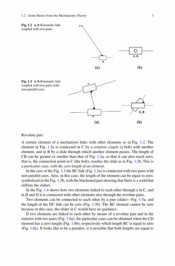
Fig. 1.2 a, b Kinematic linkcoupled with two pairs
Fig. 1.3 a, b Kinematic linkcoupled with two pairs withnon-parallel axes
Revolute pair:
A certain element of a mechanism links with other elements as in Fig. 1.2. Theelement in Fig. 1.2a is connected in C by a rotation couple (a bolt) with anotherelement, and in B by a slide through which another element passes. The length ofCB can be greater or smaller than that of Fig. 1.2a, so that it can also reach zero,that is, the connection point in C (the bolt), reaches the slide as in Fig. 1.2b. This isa particular case, with the zero length of an element.
In the case of the Fig. 1.3 the BC link (Fig. 1.3a) is connected with two pairs withnon-parallel axes. Also, in this case, the length of the element can be equal to zero,symbolized in the Fig. 1.3b, with the blackened part showing that there is a weld thatstiffens the sliders.
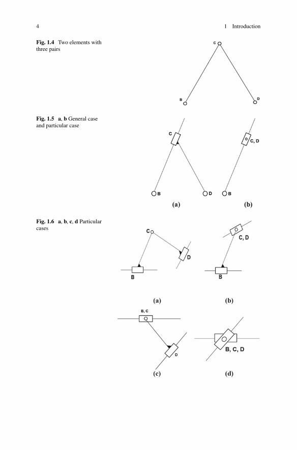
In the Fig. 1.4 shows how two elements linked to each other through a in C, andin B and D it is connected with other elements also through the revolute pairs.
Two elements can be connected to each other by a pair (slide)—Fig. 1.5a, andthe length of the DC link can be zero (Fig. 1.5b). The BC element cannot be zerobecause in this case, the slider in C would have no guidance.
If two elements are linked to each other by means of a revolute pair and in theexterior with two pairs (Fig. 1.6a), the particular cases can be obtained when the CDelement has a zero length (Fig. 1.6b), respectively which length BC is equal to zero(Fig. 1.6c). It looks like to be a paradox; it is possible that both lengths are equal to
4 1 Introduction
Fig. 1.4 Two elements withthree pairs
Fig. 1.5 a, b General caseand particular case
Fig. 1.6 a, b, c, d Particularcases
1.2 Some Basics from the Mechanisms Theory 5
zero (Fig. 1.6d). The prismatic pairs are rotated to each other and two other elementsare moved through their guidelines [2, 3].
The sequence of elements and pairs form a kinematic chain.The geometry is used for the calculations required to find geometric places. This
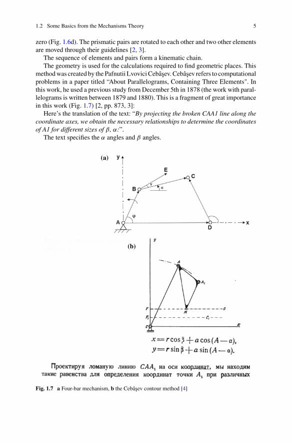
methodwas created by the Pafnutii Lvovici Cebâsev. Cebâsev refers to computationalproblems in a paper titled “About Parallelograms, Containing Three Elements". Inthis work, he used a previous study fromDecember 5th in 1878 (the work with paral-lelograms is written between 1879 and 1880). This is a fragment of great importancein this work (Fig. 1.7) [2, pp. 873, 3]:
Here’s the translation of the text: “By projecting the broken CAA1 line along thecoordinate axes, we obtain the necessary relationships to determine the coordinatesof A1 for different sizes of β, α:”.
The text specifies the α angles and β angles.
(a)
(b)
Fig. 1.7 a Four-bar mechanism, b the Cebâsev contour method [4]
6 1 Introduction
Here’s how this method applies to the mechanism given in Fig. 1.7, (called thearticulated quadrilateral mechanisms). We consider the kinematic elements of themechanism as vectors and the vector contours are projected on the system axes.There are two vector outlines reaching the point C: ABC and ADC, which, on axes,lead to the nonlinear algebraic system given by Eqs. 1.1 and 1.2, from which theangles are calculated. In order to find the trajectory of an E-point belonging to theECB element, the EA outline is projected onto the axes to obtain relations Eqs. 1.3and 1.4, that is, the coordinates of the traversing point. This leads to a first locusproblem: to find the geometric location of the point E of an ECB plate element thatmoves with points B and C on two circles.
AB cosϕ + BC cosα = AD + DC cosβ (1.1)
AB sinϕ + BC sinα = DC sinβ (1.2)
xE = AB cosϕ + BE cos(α + γ ) (1.3)
yE = AB sinϕ + BE sin(α + γ ) (1.4)
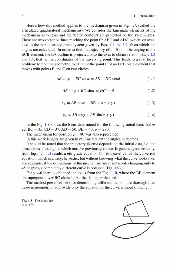
In the Fig. 1.8 shows the locus determined for the following initial data: AB =22; BC = 35; CD = 37; AD = 50; BE = 40; γ = 270.
The mechanism for position ϕ = 80 was also represented.In this work lenghts are given in millimeters ant the angles in degrees.It should be noted that the trajectory (locus) depends on the initial data, i.e. the
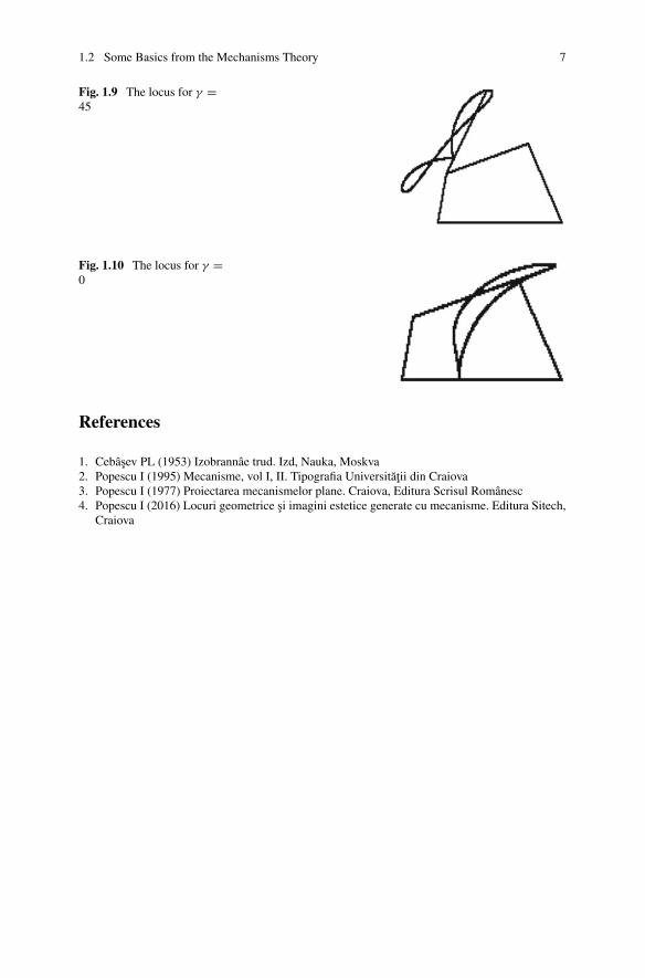
dimensions of the figure, whichmust be previously known. In general, geometrically,from Eqs. 1.1–1.4 results a 6th-grade equation (for this case) called the curve rodequation, which is a tricyclic sextic, but without knowing what the curve looks like.For example, if the dimensions of the mechanism are maintained, changing only to45 degrees, a completely different curve is obtained (Fig. 1.9).
For γ =0 there is obtained the locus from the Fig. 1.10, where the BE elementare superposed over BC element, but that is longer than this.
The method presented here for determining different loci is more thorough thanthose in geometry that provide only the equation of the curve without showing it.
Fig. 1.8 The locus forγ = 270
1.2 Some Basics from the Mechanisms Theory 7
Fig. 1.9 The locus for γ =45
Fig. 1.10 The locus for γ =0
References
1. Cebâsev PL (1953) Izobrannâe trud. Izd, Nauka, Moskva2. Popescu I (1995) Mecanisme, vol I, II. Tipografia Universitatii din Craiova3. Popescu I (1977) Proiectarea mecanismelor plane. Craiova, Editura Scrisul Românesc4. Popescu I (2016) Locuri geometrice si imagini estetice generate cu mecanisme. Editura Sitech,
Craiova

Chapter 2Loci Generated by the Point of a LineWhich Moves One End on a Circleand the Other on a Line
Abstract We start from a simple geometric problem, when a straight line slideswith one end on a circle and the other on a straight line (both fixed) and we look forthe trajectory of a point on this straight line. We construct the equivalent mechanismwhich is the rod-crank mechanism, we write the relationships for the positions, wedraw the mechanism in several positions and then we obtaine a succession of thecurves generated by the points on this line. The case is generalized by replacing thefixed linewith amobile one, resulting a lot of curves, variable depending on the corre-lation of the angles of the two leading elements. The resulting curves are differentfrom one case to another, being open curves and some having several branches[1, 2] (Luca et al. in Studies regarding of aesthetics surfaces with mechnanisms.In: Mathematical Methods for Information Science and Economics. Proceedings ofthe 17th WSEAS International Conference on Applied Mathematics (AMATH ‘12),Montreux, Switzerland, pp. 249–254, 2012; Sass et al. in J Ind Design Eng Graphics.Papers of the International Conference on Engineering Graphics and Design, Sect. 3:Engineering Computer Graphics, Nr. 12, (1):41–46, 2017).
• Case 1
The line BC in Fig. 2.1 has end B moving on a circle, and end C on a fixed line, EC.The resulting mechanism, given in Fig. 2.2 is of the type R-RRP, i.e. the connectingrod-crank mechanism extensively studied in the works on mechanisms [3] [Note:R—rotation coupling that allows only one element to rotate in relation to the other,P—prismatic torque, which allows only one translation between two elements].
The following relations are written:
xB = xA + AB cosϕ (2.1)
yB = yA + AB sinϕ (2.2)
© The Author(s), under exclusive license to Springer Nature Switzerland AG 2021I. Popescu et al., Problems of Locus Solved by Mechanisms Theory,Springer Tracts in Mechanical Engineering,https://doi.org/10.1007/978-3-030-63079-9_2
9
10 2 Loci Generated by the Point of a Line Which Moves …
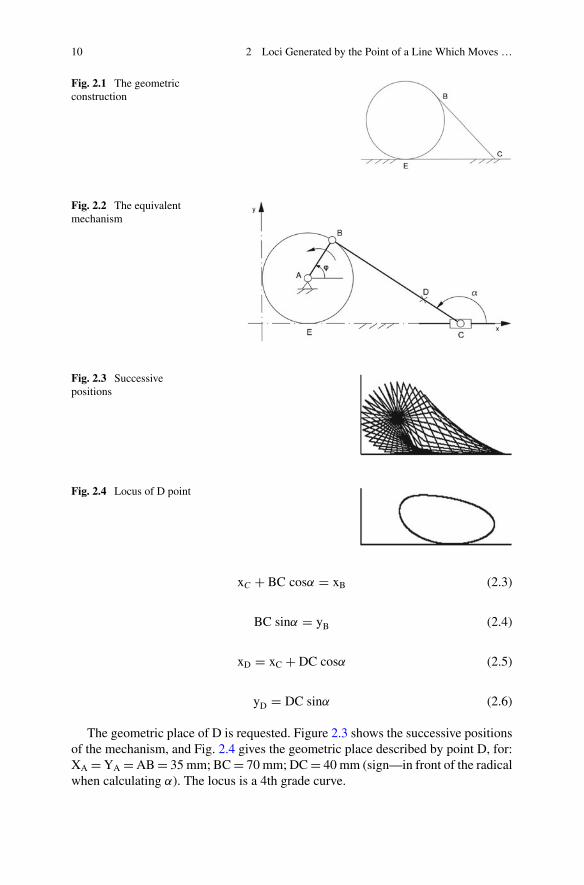
Fig. 2.1 The geometricconstruction
Fig. 2.2 The equivalentmechanism
Fig. 2.3 Successivepositions
Fig. 2.4 Locus of D point
xC + BC cosα = xB (2.3)
BC sinα = yB (2.4)
xD = xC + DC cosα (2.5)
yD = DC sinα (2.6)
The geometric place of D is requested. Figure 2.3 shows the successive positionsof the mechanism, and Fig. 2.4 gives the geometric place described by point D, for:XA =YA =AB= 35 mm; BC= 70 mm; DC= 40 mm (sign—in front of the radicalwhen calculating α). The locus is a 4th grade curve.
2 Loci Generated by the Point of a Line Which Moves … 11
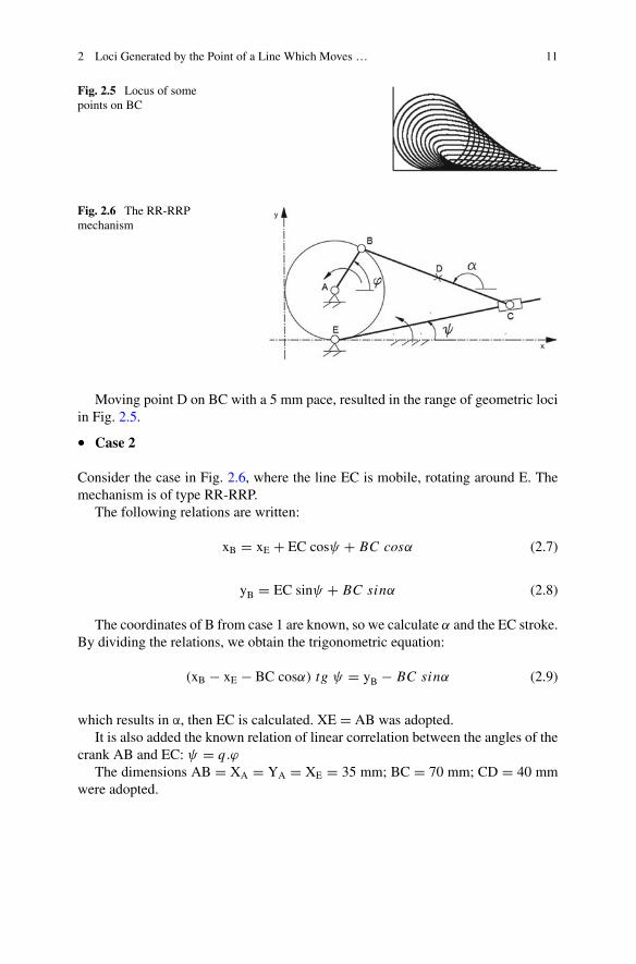
Fig. 2.5 Locus of somepoints on BC
Fig. 2.6 The RR-RRPmechanism
Moving point D on BC with a 5 mm pace, resulted in the range of geometric lociin Fig. 2.5.
• Case 2
Consider the case in Fig. 2.6, where the line EC is mobile, rotating around E. Themechanism is of type RR-RRP.
The following relations are written:
xB = xE + EC cosψ + BC cosα (2.7)
yB = EC sinψ + BC sinα (2.8)
The coordinates of B from case 1 are known, so we calculate α and the EC stroke.By dividing the relations, we obtain the trigonometric equation:
(xB − xE − BC cosα) tg ψ = yB − BC sinα (2.9)
which results in α, then EC is calculated. XE = AB was adopted.It is also added the known relation of linear correlation between the angles of the
crank AB and EC: ψ = q.ϕ
The dimensions AB = XA = YA = XE = 35 mm; BC = 70 mm; CD = 40 mmwere adopted.
12 2 Loci Generated by the Point of a Line Which Moves …
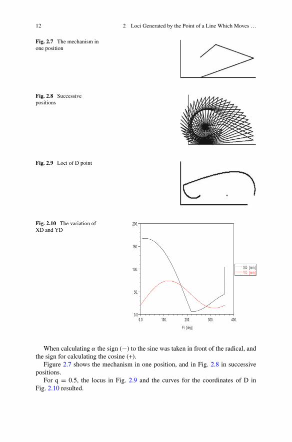
Fig. 2.7 The mechanism inone position
Fig. 2.8 Successivepositions
Fig. 2.9 Loci of D point
Fig. 2.10 The variation ofXD and YD
0.0 100. 200. 300. 400.
Fi [ deg]
0.0
50.
100.
150.
200.
X D [mm ]Y D [mm ]
When calculating α the sign (−) to the sine was taken in front of the radical, andthe sign for calculating the cosine (+).
Figure 2.7 shows the mechanism in one position, and in Fig. 2.8 in successivepositions.
For q = 0.5, the locus in Fig. 2.9 and the curves for the coordinates of D inFig. 2.10 resulted.

2 Loci Generated by the Point of a Line Which Moves … 13
Fig. 2.11 q = 0.02
Fig. 2.12 q = −0.02
Fig. 2.13 q = 0.05
Fig. 2.14 q = −0.05
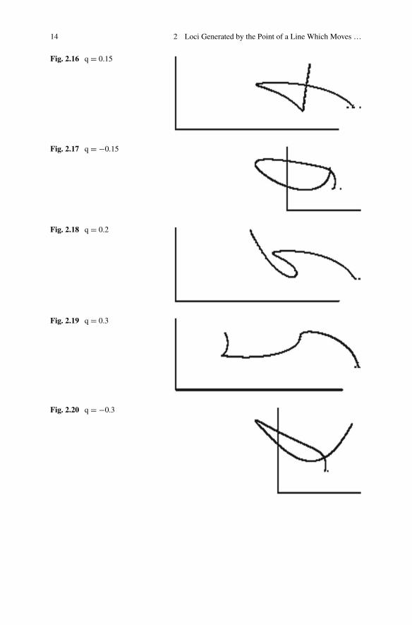
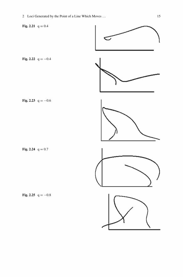
Next, the resulting loci for point D are given at different values of the correlationcoefficient q both positive (AB and EC rotate in the same direction) and negative(AB and EC rotate in the opposite direction) (Figs. 2.11, 2.12, 2.13, 2.14, 2.15, 2.16,2.17, 2.18, 2.19, 2.20, 2.21, 2.22, 2.23, 2.24, 2.25, 2.26, 2.27, 2.28, 2.29, and 2.30).
It is found that they have loci with one or more branches, all being open curves.
Fig. 2.15 q = 0.09
14 2 Loci Generated by the Point of a Line Which Moves …
Fig. 2.16 q = 0.15
Fig. 2.17 q = −0.15
Fig. 2.18 q = 0.2
Fig. 2.19 q = 0.3
Fig. 2.20 q = −0.3
2 Loci Generated by the Point of a Line Which Moves … 15
Fig. 2.21 q = 0.4
Fig. 2.22 q = −0.4
Fig. 2.23 q = −0.6
Fig. 2.24 q = 0.7
Fig. 2.25 q = −0.8

16 2 Loci Generated by the Point of a Line Which Moves …
Fig. 2.26 q = 1
Fig. 2.27 q = −1
Fig. 2.28 q = 1.5
Fig. 2.29 q = 2
Fig. 2.30 q = −2
References 17
References
1. Calbureanu M, Malciu R, Lungu M, Calbureanu D (May, 2008) The influence of the lubricantfrom a rectilinear pair above the work accuracy of the elastic elements from the high precisionmechanisms. Appl Theoret Mech Manuscript 3(5):176–185, ISSN: 1991–8747 (received Oct.16, 2007) (revised Apr. 18, 2008)
2. Luca L, Popescu I, Ghimis S (December, 2012) Studies regarding of aesthetics surfaces withmechnanisms. In : Mathematical methods for information science and economics. Proceedingsof the 17th WSEAS international conference on applied mathematics (AMATH ‘12), pp 29–31,pp 249–254. Montreux, Switzerland
3. Sass L, Duta A, Popescu I (2017) Nature gives us beauty, insoiring the technical creativity. J IndDesign Eng Graphics (1):41–46. Papers of the international conference on engineering graphicsand design, section 3: engineering computer graphics, Nr. 12
Chapter 3Loci Generated by the Pointof Intersection of Two Lines
Abstract We consider two straight lines (cranks) with one end fixed at the base(frame) and we are looking for the trajectory of their intersection point when bothstraight lines rotate. The mechanism is constructed for the case when a line has afinite length and shows the successive positions and the trajectory of their inter-section point [1], which is an incomplete circle. Both straight lines with infinitelengths are considered, resulting another equivalent mechanism with two leadingelements. Depending on the correlation between the angles of rotation of these lines,many trajectories result, some being known curves, others unknown [3], with severalincomplete branches [2]. The successive positions of the equivalent mechanism arealso given. In another case, one of the lines is no longer connected to the base by aR coupling, but by a P coupling, so it slides on a fixed line. Numerous successivecurves and positions are also obtained. Another case has in B only two couplings,the trajectory being a straight line.
• Case 1
Consider two lines AB and BC, which rotate around the fixed points A and C and thelocus of their intersection point B is required (Fig. 3.1). The length of BC is constant.
The equivalent mechanism is given in Fig. 3.2 and is of type R—PRR.Based on Fig. 3.2 the following relations are written:
xB = AB cosϕ = xC + BC cosα (3.1)
yB = AB sinϕ = BC sinα (3.2)
We get to the equation:
(xC + BC cosα)tg ϕ = BC sinα (3.3)
© The Author(s), under exclusive license to Springer Nature Switzerland AG 2021I. Popescu et al., Problems of Locus Solved by Mechanisms Theory,Springer Tracts in Mechanical Engineering,https://doi.org/10.1007/978-3-030-63079-9_3
19

20 3 Loci Generated by the Point of Intersection of Two Lines
Fig. 3.1 The geometric construction
Fig. 3.2 The equivalent mechanism
from which the angle α results.From Fig. 3.2 it is noted that point B describes a circle around C, because BC is
constant. For BC = 50 mm and XC = 20 mm we have the circle in Fig. 3.3 and thesuccessive positions of the mechanism of Fig. 3.4. It is observed that the drawn circleis incomplete, that is the mechanism does not work in a subinterval of the cycle.
3 Loci Generated by the Point of Intersection of Two Lines 21
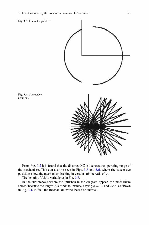
Fig. 3.3 Locus for point B
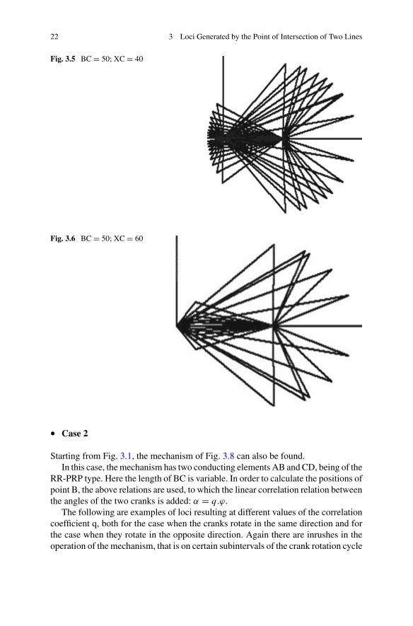
Fig. 3.4 Successivepositions
From Fig. 3.2 it is found that the distance XC influences the operating range ofthe mechanism. This can also be seen in Figs. 3.5 and 3.6, where the successivepositions show the mechanism locking in certain subintervals of ϕ.
The length of AB is variable as in Fig. 3.7.In the subintervals where the inrushes in the diagram appear, the mechanism
seizes, because the length AB tends to infinity, having ϕ = 90 and 270°, as shownin Fig. 3.4. In fact, the mechanism works based on inertia.
22 3 Loci Generated by the Point of Intersection of Two Lines
Fig. 3.5 BC = 50; XC = 40
Fig. 3.6 BC = 50; XC = 60
• Case 2
Starting from Fig. 3.1, the mechanism of Fig. 3.8 can also be found.In this case, themechanism has two conducting elements AB and CD, being of the
RR-PRP type. Here the length of BC is variable. In order to calculate the positions ofpoint B, the above relations are used, to which the linear correlation relation betweenthe angles of the two cranks is added: α = q.ϕ.
The following are examples of loci resulting at different values of the correlationcoefficient q, both for the case when the cranks rotate in the same direction and forthe case when they rotate in the opposite direction. Again there are inrushes in theoperation of the mechanism, that is on certain subintervals of the crank rotation cycle


![Paraclisul Nu0103scu0103toarei de Dumnezeu - Xenia (2)[1]. Doc (1)](https://static.fdocumente.com/doc/165x107/563dbb71550346aa9aad3921/paraclisul-nu0103scu0103toarei-de-dumnezeu-xenia-21-doc-1.jpg)