TEZA DE ABILITARE˘ Metode de Descres¸tere pe Coordonate ...141.85.225.150/papers/thesis_N.pdf ·...
186
Universitatea Politehnica Bucures ¸ti Facultatea de Automatic˘ as ¸i Calculatoare Departamentul de Automatic˘ as ¸i Ingineria Sistemelor TEZ ˘ A DE ABILITARE Metode de Descres ¸tere pe Coordonate pentru Optimizare Rar˘ a (Coordinate Descent Methods for Sparse Optimization) Ion Necoar˘ a 2013
Transcript of TEZA DE ABILITARE˘ Metode de Descres¸tere pe Coordonate ...141.85.225.150/papers/thesis_N.pdf ·...
Universitatea Politehnica BucurestiFacultatea de Automatica si Calculatoare
Departamentul de Automatica si Ingineria Sistemelor
TEZA DE ABILITARE
Metode de Descrestere pe Coordonate pentruOptimizare Rara
(Coordinate Descent Methods for Sparse Optimization)
Ion Necoara
2013

ii
.
Contents
1 Rezumat 11.1 Contributiile acestei teze . . . . . . . . . . . . . . . . . . . . . . . . . . . . . . 11.2 Principalele publicatii pe algoritmi de optimizare pe coordonate . . . . . . . . . 4
2 Summary 62.1 Contributions of this thesis . . . . . . . . . . . . . . . . . . . . . . . . . . . . . 62.2 Main publications on coordinate descent algorithms . . . . . . . . . . . . . . . . 9
3 Random coordinate descent methods for linearly constrained smooth optimization 113.1 Introduction . . . . . . . . . . . . . . . . . . . . . . . . . . . . . . . . . . . . . 113.2 Problem formulation . . . . . . . . . . . . . . . . . . . . . . . . . . . . . . . . 133.3 Previous work . . . . . . . . . . . . . . . . . . . . . . . . . . . . . . . . . . . . 143.4 Random block coordinate descent method . . . . . . . . . . . . . . . . . . . . . 153.5 Convergence rate in expectation . . . . . . . . . . . . . . . . . . . . . . . . . . 16
3.5.1 Design of probabilities . . . . . . . . . . . . . . . . . . . . . . . . . . . 213.6 Comparison with full projected gradient method . . . . . . . . . . . . . . . . . . 243.7 Convergence rate for strongly convex case . . . . . . . . . . . . . . . . . . . . . 273.8 Convergence rate in probability . . . . . . . . . . . . . . . . . . . . . . . . . . . 283.9 Random pairs sampling . . . . . . . . . . . . . . . . . . . . . . . . . . . . . . . 303.10 Generalizations . . . . . . . . . . . . . . . . . . . . . . . . . . . . . . . . . . . 31
3.10.1 Parallel coordinate descent algorithm . . . . . . . . . . . . . . . . . . . 313.10.2 Optimization problems with general equality constraints . . . . . . . . . 33
3.11 Applications . . . . . . . . . . . . . . . . . . . . . . . . . . . . . . . . . . . . . 343.11.1 Recovering approximate primal solutions from full dual gradient . . . . . 35
4 Random coordinate descent methods for singly linearly constrained smooth opti-mization 374.1 Introduction . . . . . . . . . . . . . . . . . . . . . . . . . . . . . . . . . . . . . 374.2 Problem formulation . . . . . . . . . . . . . . . . . . . . . . . . . . . . . . . . 394.3 Random block coordinate descent method . . . . . . . . . . . . . . . . . . . . . 404.4 Convergence rate in expectation . . . . . . . . . . . . . . . . . . . . . . . . . . 43
4.4.1 Choices for probabilities . . . . . . . . . . . . . . . . . . . . . . . . . . 464.5 Worst case analysis between (RCD) and full projected gradient . . . . . . . . . . 494.6 Convergence rate in probability . . . . . . . . . . . . . . . . . . . . . . . . . . 504.7 Convergence rate for strongly convex case . . . . . . . . . . . . . . . . . . . . . 504.8 Extensions . . . . . . . . . . . . . . . . . . . . . . . . . . . . . . . . . . . . . . 52
4.8.1 Generalization of algorithm (RCD) to more than 2 blocks . . . . . . . . 524.8.2 Extension to different local norms . . . . . . . . . . . . . . . . . . . . . 53
iii
Contents iv
4.9 Numerical experiments . . . . . . . . . . . . . . . . . . . . . . . . . . . . . . . 54
5 Random coordinate descent method for linearly constrained composite optimization 575.1 Introduction . . . . . . . . . . . . . . . . . . . . . . . . . . . . . . . . . . . . . 575.2 Problem formulation . . . . . . . . . . . . . . . . . . . . . . . . . . . . . . . . 585.3 Previous work . . . . . . . . . . . . . . . . . . . . . . . . . . . . . . . . . . . . 615.4 Random coordinate descent algorithm . . . . . . . . . . . . . . . . . . . . . . . 625.5 Convergence rate in expectation . . . . . . . . . . . . . . . . . . . . . . . . . . 635.6 Convergence rate for strongly convex functions . . . . . . . . . . . . . . . . . . 675.7 Convergence rate in probability . . . . . . . . . . . . . . . . . . . . . . . . . . . 695.8 Generalizations . . . . . . . . . . . . . . . . . . . . . . . . . . . . . . . . . . . 695.9 Complexity analysis and comparison with other approaches . . . . . . . . . . . 705.10 Numerical experiments . . . . . . . . . . . . . . . . . . . . . . . . . . . . . . . 74
5.10.1 Support vector machine . . . . . . . . . . . . . . . . . . . . . . . . . . 745.10.2 Chebyshev center of a set of points . . . . . . . . . . . . . . . . . . . . 765.10.3 Random generated problems with ℓ1-regularization term . . . . . . . . . 79
6 Random coordinate descent methods for nonconvex composite optimization 816.1 Introduction . . . . . . . . . . . . . . . . . . . . . . . . . . . . . . . . . . . . . 816.2 Unconstrained minimization of composite objective functions . . . . . . . . . . 83
6.2.1 Problem formulation . . . . . . . . . . . . . . . . . . . . . . . . . . . . 836.2.2 An 1-random coordinate descent algorithm . . . . . . . . . . . . . . . . 846.2.3 Convergence . . . . . . . . . . . . . . . . . . . . . . . . . . . . . . . . 866.2.4 Linear convergence for objective functions with error bound . . . . . . . 90
6.3 Constrained minimization of composite objective functions . . . . . . . . . . . . 936.3.1 Problem formulation . . . . . . . . . . . . . . . . . . . . . . . . . . . . 936.3.2 A 2-random coordinate descent algorithm . . . . . . . . . . . . . . . . . 946.3.3 Convergence . . . . . . . . . . . . . . . . . . . . . . . . . . . . . . . . 966.3.4 Constrained minimization of smooth objective functions . . . . . . . . . 100
6.4 Numerical experiments . . . . . . . . . . . . . . . . . . . . . . . . . . . . . . . 102
7 Distributed random coordinate descent methods for composite optimization 1087.1 Introduction . . . . . . . . . . . . . . . . . . . . . . . . . . . . . . . . . . . . . 1087.2 Problem formulation . . . . . . . . . . . . . . . . . . . . . . . . . . . . . . . . 109
7.2.1 Motivating practical applications . . . . . . . . . . . . . . . . . . . . . . 1137.3 Distributed and parallel coordinate descent method . . . . . . . . . . . . . . . . 1157.4 Sublinear convergence for smooth convex minimization . . . . . . . . . . . . . . 1187.5 Linear convergence for error bound convex minimization . . . . . . . . . . . . . 1217.6 Conditions for generalized error bound functions . . . . . . . . . . . . . . . . . 128
7.6.1 Case 1: f strongly convex and Ψ convex . . . . . . . . . . . . . . . . . . 1287.6.2 Case 2: Ψ indicator function of a polyhedral set . . . . . . . . . . . . . . 1297.6.3 Case 3: Ψ polyhedral function . . . . . . . . . . . . . . . . . . . . . . . 1367.6.4 Case 4: dual formulation . . . . . . . . . . . . . . . . . . . . . . . . . . 141
7.7 Convergence analysis under sparsity conditions . . . . . . . . . . . . . . . . . . 1417.7.1 Distributed implementation . . . . . . . . . . . . . . . . . . . . . . . . 1427.7.2 Comparison with other approaches . . . . . . . . . . . . . . . . . . . . . 143
7.8 Numerical simulations . . . . . . . . . . . . . . . . . . . . . . . . . . . . . . . 145

Contents v
8 Parallel coordinate descent algorithm for separable constraints optimization: appli-cation to MPC 1498.1 Introduction . . . . . . . . . . . . . . . . . . . . . . . . . . . . . . . . . . . . . 1498.2 Parallel coordinate descent algorithm (PCDM) for separable constraints mini-
mization . . . . . . . . . . . . . . . . . . . . . . . . . . . . . . . . . . . . . . . 1518.2.1 Parallel Block-Coordinate Descent Method . . . . . . . . . . . . . . . . 151
8.3 Application of PCDM to distributed suboptimal MPC . . . . . . . . . . . . . . . 1548.3.1 MPC for networked systems: terminal cost and no end constraints . . . . 1558.3.2 Distributed synthesis for a terminal cost . . . . . . . . . . . . . . . . . . 1568.3.3 Stability of the MPC scheme . . . . . . . . . . . . . . . . . . . . . . . . 158
8.4 Distributed implementation of MPC scheme based on PCDM . . . . . . . . . . . 1588.5 Numerical Results . . . . . . . . . . . . . . . . . . . . . . . . . . . . . . . . . . 159
8.5.1 Quadruple tank process . . . . . . . . . . . . . . . . . . . . . . . . . . . 1608.5.2 Implementation of the MPC scheme using MPI . . . . . . . . . . . . . . 1618.5.3 Implementation of the MPC scheme using Siemens S7-1200 PLC . . . . 1628.5.4 Implementation of MPC scheme for random networked systems . . . . . 164
9 Future Work 1669.1 Huge-scale sparse optimization: theory, algorithms and applications . . . . . . . 167
9.1.1 Methodology and capacity to generate results . . . . . . . . . . . . . . . 1689.2 Optimization based control for distributed networked systems . . . . . . . . . . . 170
9.2.1 Methodology and capacity to generate results . . . . . . . . . . . . . . . 1709.3 Optimization based control for resource-constrained embedded systems . . . . . 171
9.3.1 Methodology and capacity to generate results . . . . . . . . . . . . . . . 172
Bibliography 174
Chapter 1
Rezumat
1.1 Contributiile acestei tezePrincipala problema de optimizare considerata in aceasta teza este de urmatoarea forma:
minx∈Rn
F (x) (= f(x) + Ψ(x)) (1.1)
s.t.: Ax = b,
unde f este o functie neteda (gradient Lipschitz), Ψ este o functie de regularizare simpla (min-imizarea sumei dintre aceasta functie si una patratica este usoara) si matricea A ∈ Rm×n estede obicei rara data de structura unui graf asociat problemei. O alta caracteristica a proble-mei este dimensiunea foarte mare, adica n este de ordinul milioanelor sau miliardelor. Pre-supunem de asemenea ca variabila de decizie x poate fi descompusa in (blocuri) componentex = [xT1 xT2 . . . x
TN ]
T , unde xi ∈ Rni si∑
i ni = n. De notat este faptul ca acesta problema deoptimizare este foarte generala si apare in multe aplicatii din inginerie:
• Ψ este functia indicator a unei multimi convexe X care poate fi scrisa de obicei ca unprodus Cartezian X = X1 × X2 × · · · × XN , unde Xi ⊆ Rni . Aceasta problema estecunoscuta sub numele de problema de optimizare separabila cu restrictii de cuplare liniaresi apare in multe aplicatii din control si estimare distribuita [13,62,65,100,112], optimizarein retea [9, 22, 82, 98, 110, 121], computer vision [10, 44], etc.
• Ψ este fie functia indicator a unei multimi convexe X = X1 ×X2 × · · · ×XN sau norma1, notatata ∥x∥1 (pentru a obtine solutie rara) iar matricea A = 0. Aceasta problema aparein control predictiv distribuit [61, 103], procesare de imagine [14, 21, 47, 105], clasificare[99, 123, 124], data mining [16, 86, 119], etc.
• Ψ este functia indicator a unei multimi convexe X = X1 × X2 × · · · × XN iar A = aT ,adica avem o singura restrictie liniara de cuplare. Aceasta problema apare in ierarhizareapaginilor (problema Google) [59, 76], control [39, 83, 84, 104], invatare [16–18, 109, 111],truss topology design [42], etc.
Se observa ca (1.1) se incadreaza in clasa de probleme de optimizare de mari dimensiuni cu datesi/sau solutii rare. Abordarea standard pentru rezolvarea problemei de optimizare de dimensiunifoarte mari (1.1) se bazeaza pe descompunere. Metodele de descompunere reprezinta o unealtaeficienta pentru rezolvarea acestui tip de problema datorita faptului ca acestea permit impartireaproblemei originale de dimensiuni mari in subprobleme mici care sunt apoi coordonate de o
1
1.1 Contributiile acestei teze 2
problema master. Metodele de descompunere se impart in doua clase: descompunere primala siduala. In metodele de descompunere primala problema originala este tratata direct, in timp ce inmetodele duale restrictiile de cuplare sunt mutate in cost folosind multiplicatorii Lagrange, dupacare se rezolva problema duala. In activitatea mea de cercetare din ultimii 7 ani am dezvoltatsi analizat algoritmi apartinand ambelor clase de metode de descompunere. Din cunostintelemele am fost printre primii cercetatori care au folosit tehnicile de netezire in descompunereaduala pentru a obtine rate de convergenta mai rapide pentru algoritmii duali propusi (vezilucrarile [64, 65, 71, 72, 90, 91, 110]). Totusi, in aceasta teza am optat pentru prezentarea celormai recente rezultate obtinute de mine pentru metodele de descompunere primala, si anumemetodele de descrestere pe coordonate (vezi lucrarile [59–61, 65, 67, 70, 84]). Principalelecontributii ale acestei teze, pe capitole, sunt urmatoarele:
Capitol 3: In acest capitol dezvoltam metode aleatoare de descrestere pe coordonate pentruminimizarea problemelor de optimizare convexa de dimensiuni foarte mari supuse la con-strangeri liniare de cuplare si avand functia obiectiv cu gradient Lipschitz pe coordonate.Deoarece avem constrangeri de cuplare in problema de optimizare, trebuie sa definim unalgoritm care actualizeaza doua (blocuri) componente pe iteratie. Demonstram ca pentru acestemetode se obtine o ϵ-aproximativ solutie in valoarea medie a functiei obiectiv in cel multO(1
ϵ) iteratii. Pe de alta parte, complexitatea numerica a fiecarei iteratii este mult mai mica
decat a metodelor bazate pe intreg gradientul. Ne concentram de asemenea atentia pe alegereaoptima a probabilitatilor pentru a face acesti algoritmi sa convearga rapid si demonstram caaceasta conduce la rezolvarea unei probleme SDP rare si de mici dimensiuni. Analiza ratei deconvergenta in probabilitate este de asemenea data in acest capitol. Pentru functii obiectiv tariconvexe aratam ca noii algoritmi converg liniar. Extindem de asemena algoritmul principal, incare se actualizeaza o singura componenta (bloc), la un algorithm paralel in care se updateazamai multe (blocuri de) componente pe iteratie si aratam ca pentru aceasta versiune paralelarata de convergenta depinde liniar de numarul de (blocuri) componente actualizate. Testelenumerice confirma ca pe probleme de optimizare de largi dimensiuni, pentru care calculareaunei componente a gradientului este usoara din punct de vedere numeric, noile metode propusesunt mult mai eficiente decat metodele bazate pe intreg gradientul. Acest capitol se bazeaza pearticolele [67, 68].
Capitol 4: In acest capitol dezvoltam metode aleatoare de descrestere pe coordonate pentruminimizarea problemelor de optimizare convexa multi-agent avand functia obiectiv cu gradientLipschitz pe coordonate si cu o singura constrangere de cuplare. Datorita prezentei constrangeriide cuplare in problema de optimizare, algoritmii prezentati sunt de descrestere pe doua coordo-nate. Pentru astfel de metode demonstram ca in valoarea medie a functiei obiectiv putem obtineo ϵ-aproximativ solutie in cel mult O( 1
λ2(Q)ϵ) iteratii, unde λ2(Q) este cea de-a doua valoare
proprie a unei matrici Q definita in termeni de probabilitatile alese si numarul de blocuri. Pede alta parte, complexitatea numerica per iteratie a metodelor noastre este mult mai mica decata celor bazate pe intreg gradientul iar fiecare iteratie poate fi calculata intr-un mod distribuit.Analizam de asemenea posibilitatea alegerii optime a probabilitatilor si aratam ca aceastaanaliza conduce la rezolvarea unei probleme SDP rare. Pentru metodele dezvoltate prezentam siratele de convergenta in probabilitate. In cazul functiilor tari convexe aratam ca noii algoritmi auconvergenta liniara. Prezentam de asemenea o versiune paralela a algoritmului principal, undeactualizam mai multe (blocuri de) componente pe iteratie, pentru care derivam de asemenearata de convergenta. Algoritmii dezvoltati au fost implementati in Matlab pentru rezolvareaproblemei Google iar rezultatele din simulari arata superioritatea acestora fata de metodele
1.1 Contributiile acestei teze 3
bazate pe informatie de intreg gradient. Acest capitol se bazeaza pe lucrarile [58, 59, 69].
Capitol 5: In acest capitol propunem o varianta a unei metode aleatoare de descrestere pe coor-donate pentru rezolvarea problemelor de optimizare convexa cu funtia obiectiv de tip composite(compusa dintr-o functie convexa, cu gradient Lipschitz pe coordonate si o functie convexa, custructura simpla, dar posibil nediferentiabila) si constrangeri liniare de cuplare. Daca parteaneteda a functiei obiectiv are gradient Lipschitz pe coordonate, atunci metoda propusa alegealeator doua (blocuri) componente si obtine o ϵ-aproximativ solutie in valoarea medie a functieiobiectiv in O(N2/ϵ) iteratii, unde N este numarul de (blocuri) componente. Pentru probleme deoptimizare avand complexitate numerica mica pentru evaluarea unei componente a gradientului,metoda propusa este mai eficienta decat metodele bazate pe intreg gradientul. Analiza rateide convergenta in probabilitate este de asemenea data in acest capitol. Pentru functii obiectivtari convexe aratam ca noii algoritmi converg liniar. Algoritmul propus a fost implementat incod C si testat pe date reale de SVM si pe problema gasirii centrului Chebyshev corespunzatorunei multimi de puncte. Experimentele numerice confirma ca pe problemele de dimensiunimari metoda noastra este mai eficienta decat metodele bazate pe intreg gradientul sau metodelegreedy de descrestere pe coordonate. Acest capitol se bazeaza pe lucrarea [70].
Capitol 6: In acest capitol analizam noi metode aleatoare de descrestere pe coordonate pentrurezolvarea problemelor de optimizare neconvexe cu funtia obiectiv de tip composite: compusadintr-o functie neconvexa dar cu gradient Lipschitz pe coordonate si o functie convexa, custructura simpla, dar posibil nediferentiabila. De asemenea abordam ambele cazuri: neconstransdar si cu constrangeri liniare de cuplare. Pentru problemele de optimizare cu structura definitamai sus, propunem metode aleatoare de descrestere pe coordonate si analizam proprietatilede convergenta ale acestora. In cazul general, demonstram pentru sirurile generate de noiialgoritmi convergenta asimptotica la punctele stationare si rata de convergenta subliniara invaloarea medie a unei anumite functii masura de optimalitate. In plus, daca functia obiectivsatisface o anumita conditie de marginire a erorii de optimalitate, derivam convergenta localaliniara in valoarea medie a functiei obiectiv. Prezentam de asemenea experimente numericepentru evaluarea performantelor practice ale algoritmilor propusi pe binecunoscuta problema decomplementaritate a valorii proprii. Din experimentele numerice se observa ca pe problemele dedimensiuni mari metoda noastra este mai eficienta decat metodele bazate pe intreg gradientul.Acest capitol se bazeaza pe lucrarile [84, 85].
Capitol 7: In acest capitol propunem o versiune distribuita a unei metode aleatoare de de-screstere pe coordonate pentru minimizarea unei functii obiectiv de tip composite: compusadintr-o functie neteda convexa, partial separabila si una total separabila, convexa, dar posibilnediferentiabila. Sub ipoteza de gradient Lipschitz a partii netede, aceasta metoda are o ratade convergenta subliniara. Rata de convergenta liniara se obtine pentru o clasa nou introdusade functii obiectiv ce satisface o conditie generalizata de marginire a erorii de optimalitate.Aratam ca in noua clasa de functii se regasesc functii deja studiate, cum ar fi clasa de functiitari convexe sau clasa de functii ce satisface conditia de marginire a erorii de optimalitateclasica. Demonstram de asemenea, ca estimarile teoretice ale ratelor de convergenta depindliniar de numarul de (blocuri) componente alese aleator si de o masura a separabilitatii functieiobiectiv. Algoritmul propus a fost implementat in cod C si testat pe problema lasso constransa.Experimentele numerice confirma ca prin paralelizare se poate accelera substantial rata deconvergenta a metodei clasice de descrestere pe coordonate. Acest capitol se bazeaza pelucrarea [60].
1.2 Principalele publicatii pe algoritmi de optimizare pe coordonate 4
Capitol 8: In acest capitol propunem un algoritm paralel de descrestere pe coordonate pentrurezolvarea problemelor de optimizare convexa cu restrictii separabile ce pot aparea de exempluin controlul predictiv distribuit bazat pe model (MPC) pentru sisteme liniare de tip retea. Al-goritmul nostru se bazeaza pe actualizarea in paralel pe coordonate si are iteratia foarte simpla.Demonstram rata de convergenta liniara (subliniara) pentru sirul generat de noul algoritm subipoteze standard pentru functia obiectiv. Mai mult, algoritmul foloseste informatie locala pen-tru actualizarea componentelor variabilei de decizie si astfel este adecvat pentru implementaredistribuita. Avand, de asemenea complexitatea iteratiei mica, este potrivit pentru controlul detip embedded. Propunem o metoda de control de tip MPC bazata pe acest algoritm, pentru carefiecare subsistem din retea poate calcula intrari fezabile si stabilizatoare folosind calcule ieftinesi distribuite. Metoda de control propusa a fost implementata pe un PLC Siemens in scopulcontrolului unei instalatii reale cu patru rezervoare. Acest capitol se bazeaza pe lucrarea [61].
1.2 Principalele publicatii pe algoritmi de optimizare pe coor-donate
Rezultatele prezentate in aceasta teza au fost acceptate spre publicare in reviste ISI de top sauconferinte de prestigiu. O parte din rezultate (Capitolul 7) au fost trimise recent la reviste.Prezentam mai jos lista de publicatii pe care se bazeaza aceasta teza.
Articole in reviste ISI
• I. Necoara and D. Clipici, Distributed random coordinate descent methods for compositeminimization, partially accepted in SIAM Journal of Optimization, pp. 1–40, December2013.
• A. Patrascu and I. Necoara, Random coordinate descent methods for l0 regularized convexoptimization, accepted in IEEE Transactions on Automatic Control, to appear, 2014.
• I. Necoara, Random coordinate descent algorithms for multi-agent convex optimizationover networks, IEEE Transactions on Automatic Control, vol. 58, no. 8, pp. 1–12, 2013.
• A. Patrascu, I. Necoara, Efficient random coordinate descent algorithms for large-scalestructured nonconvex optimization, Journal of Global Optimization, DOI: 10.1007/s10898-014-0151-9, 1-32, 2014.
• I. Necoara. A. Patrascu, A random coordinate descent algorithm for optimization prob-lems with composite objective function and linear coupled constraints, Computational Op-timization and Applications, vol. 57, no. 2, pp. 307-337, 2014.
• I. Necoara, D. Clipici, Efficient parallel coordinate descent algorithm for convex opti-mization problems with separable constraints: application to distributed MPC, Journal ofProcess Control, vol. 23, no. 3, pp. 243–253, 2013.
• I. Necoara, V. Nedelcu and I. Dumitrache, Parallel and distributed optimization methodsfor estimation and control in networks, Journal of Process Control, vol. 21, no. 5, pp.756–766, 2011.
1.2 Principalele publicatii pe algoritmi de optimizare pe coordonate 5
Articole in pregatire
• I. Necoara, Y. Nesterov and F. Glineur, A random coordinate descent method on largeoptimization problems with linear constraints, Technical Report, University PolitehnicaBucharest, June 2014.
Articole in conferinte
• I. Necoara, Y. Nesterov and F. Glineur, A random coordinate descent method on largeoptimization problems with linear constraints, The Fourth International Conference onContinuous Optimization, Lisbon, 2013.
• I. Necoara, A. Patrascu, A random coordinate descent algorithm for optimization problemswith composite objective function and linear coupled constraints, The Fourth InternationalConference on Continuous Optimization, Lisbon, 2013.
• I. Necoara, D. Clipici, A computationally efficient parallel coordinate descent algorithmfor MPC implementation on a PLC, in Proceedings of 12th European Control Conference,2013
• A. Patrascu, I. Necoara, A random coordinate descent algorithm for large-scale sparsenonconvex optimization, in Proceedings of 12th European Control Conference, 2013.
• I. Necoara, Suboptimal distributed MPC based on a block-coordinate descent method withfeasibility and stability guarantees, in Proceedings of 51th IEEE Conference on Decisionand Control, 2012.
• I. Necoara, A random coordinate descent method for large-scale resource allocation prob-lems, in Proceedings of 51th IEEE Conference on Decision and Control, 2012.
• I. Necoara, A Patrascu, A random coordinate descent algorithm for singly linear con-strained smooth optimization, in Proceedings of 20th Mathematical Theory of Networkand Systems, 2012.

Chapter 2
Summary
2.1 Contributions of this thesisThe main optimization problem of interest considered in this thesis has the following form:
minx∈Rn
F (x) (= f(x) + Ψ(x)) (2.1)
s.t.: Ax = b,
where f is a smooth function (i.e. with Lipschitz gradient), Ψ is a simple convex function (i.e.minimization of the sum of this function with a quadratic term is easy) and matrix A ∈ Rm×n
is usually sparse according to some graph structure. Another characteristic of this problem is itsvery large dimension, i.e. n is very large, in particular we deal with millions or even billionsof variables. We further assume that the decision variable x can be decomposed in (block)components x = [xT1 xT2 . . . x
TN ]
T , where xi ∈ Rni and∑
i ni = n. Note that this problemis very general and appears in many engineering applications:
• Ψ is the indicator function of some convex set X that can be written usually as a Cartesianproduct X = X1 × X2 × · · · × XN , where Xi ⊆ Rni . This problem is known in theliterature as separable optimization problem with linear coupling constraints and appearsin many applications from distributed control and estimation [13,62,65,100,112], networkoptimization [9, 22, 82, 98, 110, 121], computer vision [10, 44], etc.
• Ψ is either the indicator function of some convex set X = X1 × X2 × · · · × XN or 1-norm ∥x∥1 (in order to induce sparsity in the solution) and matrix A = 0. This problemappears in distributed model predictive control [61,103], image processing [14,21,47,105],classification [99, 123, 124], data mining [16, 86, 119], etc.
• Ψ is the indicator function of some convex set X = X1 × X2 × · · · × XN and A = aT ,i.e. a single linear coupled constraint. This problem appears is page ranking (also knownas Google problem) [59, 76], control [39, 83, 84, 104], learning [16–18, 109, 111], trusstopology design [42], etc.
We notice that (2.1) belongs to the class of large-scale optimization problems with sparsedata/solutions. The standard approach for solving the large-scale optimization problem (2.1)is to use decomposition. Decomposition methods represent a powerful tool for solving thesetype of problems due to their ability of dividing the original large-scale problem into smallersubproblems which are coordinated by a master problem. Decomposition methods can be
6
2.1 Contributions of this thesis 7
divided in two main classes: primal and dual decomposition. While in the primal decompositionmethods the optimization problem is solved using the original formulation and variables, in dualdecomposition the constraints are moved into the cost using the Lagrange multipliers and thedual problem is solved. In the last 7 years I have pursued both approaches in my research. Frommy knowledge I am one of the first researchers that used smoothing techniques in Lagrangiandual decomposition in order to obtain faster convergence rates for the corresponding algorithms(see e.g. the papers [64, 65, 71, 72, 90, 91, 110]). In this thesis however, I have opted to presentsome of my recent results on primal decomposition, namely coordinate descent methods (seee.g. the papers [59–61, 65, 67, 70, 84]). The main contributions of this thesis, by chapters, are asfollows:
Chapter 3: In this chapter we develop random (block) coordinate descent methods forminimizing large-scale convex problems with linearly coupled constraints and prove thatit obtains in expectation an ϵ-accurate solution in at most O(1
ϵ) iterations. Since we have
coupled constraints in the problem, we need to devise an algorithm that updates randomlytwo (block) components per iteration. However, the numerical complexity per iteration of thenew methods is usually much cheaper than that of methods based on full gradient information.We focus on how to choose the probabilities to make the randomized algorithm to convergeas fast as possible and we arrive at solving sparse SDPs. Analysis for rate of convergencein probability is also provided. For strongly convex functions the new methods convergelinearly. We also extend the main algorithm, where we update two (block) components periteration, to a parallel random coordinate descent algorithm, where we update more than two(block) components per iteration and we show that for this parallel version the convergencerate depends linearly on the number of (block) components updated. Numerical tests confirmthat on large optimization problems with cheap coordinate derivatives the new methods aremuch more efficient than methods based on full gradient. This chapter is based on papers [67,68].
Chapter 4: In this chapter we develop randomized block-coordinate descent methods forminimizing multi-agent convex optimization problems with a single linear coupled constraintover networks and prove that they obtain in expectation an ϵ accurate solution in at mostO( 1
λ2(Q)ϵ) iterations, where λ2(Q) is the second smallest eigenvalue of a matrix Q that is defined
in terms of the probabilities and the number of blocks. However, the computational complexityper iteration of our methods is much simpler than the one of a method based on full gradientinformation and each iteration can be computed in a completely distributed way. We focus onhow to choose the probabilities to make these randomized algorithms to converge as fast aspossible and we arrive at solving a sparse SDP. Analysis for rate of convergence in probabilityis also provided. For strongly convex functions our distributed algorithms converge linearly. Wealso extend the main algorithm to a parallel random coordinate descent method and to problemswith more general linearly coupled constraints for which we also derive rate of convergence.The new algorithms were implemented in Matlab and applied for solving the Google problem,and the simulation results show the superiority of our approach compared to methods based onfull gradient. This chapter is based on papers [58, 59, 69].
Chapter 5: In this chapter we propose a variant of the random coordinate descent method forsolving linearly constrained convex optimization problems with composite objective functions.If the smooth part of the objective function has Lipschitz continuous gradient, then we provethat our method obtains an ϵ-optimal solution in O(N2/ϵ) iterations, where N is the number ofblocks. For the class of problems with cheap coordinate derivatives we show that the new method
2.1 Contributions of this thesis 8
is faster than methods based on full-gradient information. Analysis for the rate of convergence inprobability is also provided. For strongly convex functions our method converges linearly. Theproposed algorithm was implemented in code C and tested on real data from SVM and on theproblem of finding the Chebyshev center for a set of points. Extensive numerical tests confirmthat on very large problems, our method is much more numerically efficient than methods basedon full gradient information or coordinate descent methods based on greedy index selection.This chapter is based on paper [70].
Chapter 6: In this chapter we analyze several new methods for solving nonconvex optimizationproblems with the objective function formed as a sum of two terms: one is nonconvex andsmooth, and another is convex but simple and its structure is known. Further, we consider bothcases: unconstrained and linearly constrained nonconvex problems. For optimization problemsof the above structure, we propose random coordinate descent algorithms and analyze theirconvergence properties. For the general case, when the objective function is nonconvex andcomposite we prove asymptotic convergence for the sequences generated by our algorithms tostationary points and sublinear rate of convergence in expectation for some optimality measure.Additionally, if the objective function satisfies an error bound condition we derive a locallinear rate of convergence for the expected values of the objective function. We also presentextensive numerical experiments on the eigenvalue complementarity problem for evaluatingthe performance of our algorithms in comparison with state-of-the-art methods. From thenumerical experiments we can observe that on large optimization problems the new methods aremuch more efficient than methods based on full gradient. This chapter is based on papers [84,85].
Chapter 7: In this chapter we propose a distributed version of a randomized (block) coordinatedescent method for minimizing the sum of a partially separable smooth convex function anda fully separable non-smooth convex function. Under the assumption of block Lipschitzcontinuity of the gradient of the smooth function, this method is shown to have a sublinearconvergence rate. Linear convergence rate of the method is obtained for the newly introducedclass of generalized error bound functions. We prove that the new class of generalized errorbound functions encompasses both global/local error bound functions and smooth stronglyconvex functions. We also show that the theoretical estimates on the convergence rate dependon the number of blocks chosen randomly and a natural measure of separability of the objectivefunction. The new algorithm was implemented in code C and tested on the constrained lassoproblem. Numerical experiments show that by parallelization we can accelerate substantially therate of convergence of the classical random coordinate descent method. This chapter is based onpaper [60].
Chapter 8: In this chapter we propose a parallel coordinate descent algorithm for solving smoothconvex optimization problems with separable constraints that may arise e.g. in distributed modelpredictive control (MPC) for linear networked systems. Our algorithm is based on block coor-dinate descent updates in parallel and has a very simple iteration. We prove (sub)linear rate ofconvergence for the new algorithm under standard assumptions for smooth convex optimization.Further, our algorithm uses local information and thus is suitable for distributed implementations.Moreover, it has low iteration complexity, which makes it appropriate for embedded control. AnMPC scheme based on this new parallel algorithm is derived, for which every subsystem in thenetwork can compute feasible and stabilizing control inputs using distributed and cheap compu-tations. For ensuring stability of the MPC scheme, we use a terminal cost formulation derivedfrom a distributed synthesis. The proposed control method was q implemented on a PLC Siemens
2.2 Main publications on coordinate descent algorithms 9
for controlling a four tank process. This chapter is based on paper [61].
2.2 Main publications on coordinate descent algorithmsMost of the material that is presented in this thesis has been published, or accepted for publi-cation, in top journals or conference proceedings. Some of the material (Chapter 7) has beensubmitted for publication recently. We detail below the main publications from this thesis.
Articles in ISI journals
• I. Necoara and D. Clipici, Distributed random coordinate descent methods for compositeminimization, partially accepted in SIAM Journal of Optimization, pp. 1–40, December2013.
• A. Patrascu and I. Necoara, Random coordinate descent methods for l0 regularized convexoptimization, accepted in IEEE Transactions on Automatic Control, to appear, 2014.
• I. Necoara, Random coordinate descent algorithms for multi-agent convex optimizationover networks, IEEE Transactions on Automatic Control, vol. 58, no. 8, pp. 1–12, 2013.
• A. Patrascu, I. Necoara, Efficient random coordinate descent algorithms for large-scalestructured nonconvex optimization, Journal of Global Optimization, DOI: 10.1007/s10898-014-0151-9, 1-32, 2014.
• I. Necoara. A. Patrascu, A random coordinate descent algorithm for optimization prob-lems with composite objective function and linear coupled constraints, Computational Op-timization and Applications, vol. 57, no. 2, pp. 307-337, 2014.
• I. Necoara, D. Clipici, Efficient parallel coordinate descent algorithm for convex opti-mization problems with separable constraints: application to distributed MPC, Journal ofProcess Control, vol. 23, no. 3, pp. 243–253, 2013.
• I. Necoara, V. Nedelcu and I. Dumitrache, Parallel and distributed optimization methodsfor estimation and control in networks, Journal of Process Control, vol. 21, no. 5, pp.756–766, 2011.
Articles in preparation
• I. Necoara, Y. Nesterov and F. Glineur, A random coordinate descent method on largeoptimization problems with linear constraints, Technical Report, University PolitehnicaBucharest, June 2014.
Articles in conferences
• I. Necoara, Y. Nesterov and F. Glineur, A random coordinate descent method on largeoptimization problems with linear constraints, The Fourth International Conference onContinuous Optimization, Lisbon, 2013.
• I. Necoara, A. Patrascu, A random coordinate descent algorithm for optimization problemswith composite objective function and linear coupled constraints, The Fourth InternationalConference on Continuous Optimization, Lisbon, 2013.
2.2 Main publications on coordinate descent algorithms 10
• I. Necoara, D. Clipici, A computationally efficient parallel coordinate descent algorithmfor MPC implementation on a PLC, in Proceedings of 12th European Control Conference,2013
• A. Patrascu, I. Necoara, A random coordinate descent algorithm for large-scale sparsenonconvex optimization, in Proceedings of 12th European Control Conference, 2013.
• I. Necoara, Suboptimal distributed MPC based on a block-coordinate descent method withfeasibility and stability guarantees, in Proceedings of 51th IEEE Conference on Decisionand Control, 2012.
• I. Necoara, A random coordinate descent method for large-scale resource allocation prob-lems, in Proceedings of 51th IEEE Conference on Decision and Control, 2012.
• I. Necoara, A Patrascu, A random coordinate descent algorithm for singly linear con-strained smooth optimization, in Proceedings of 20th Mathematical Theory of Networkand Systems, 2012.

Chapter 3
Random coordinate descent methods forlinearly constrained smooth optimization
In this chapter we develop random block coordinate descent methods for minimizing large-scaleconvex problems with linearly coupled constraints and prove that it obtains in expectation an ϵ-accurate solution in at most O(1
ϵ) iterations. Since we have coupled constraints in the problem,
we need to devise an algorithm that updates randomly two (block) components per iteration.However, the numerical complexity per iteration of the new methods is usually much cheaper thanthat of methods based on full gradient information. We focus on how to choose the probabilities tomake the randomized algorithm to converge as fast as possible and we arrive at solving sparseSDPs. Analysis for rate of convergence in probability is also provided. For strongly convexfunctions the new methods converge linearly. We also extend the main algorithm, where weupdate two (block) components per iteration, to a parallel random coordinate descent algorithm,where we update more than two (block) components per iteration and we show that for thisparallel version the convergence rate depends linearly on the number of (block) componentsupdated. Numerical tests confirm that on large optimization problems with cheap coordinatederivatives the new methods are much more efficient than methods based on full gradient. Thischapter is based on papers [67, 68].
3.1 IntroductionThe performance of a network composed of interconnected subsystems can be increased if thetraditionally separated subsystems are jointly optimized. Recently, parallel and distributed op-timization methods have emerged as a powerful tool for solving large network optimizationproblems: e.g. resource allocation [32, 34, 121], telecommunications [8, 110], coordination inmulti-agent systems [121], estimation in sensor networks [65], distributed control [65], imageprocessing [21], traffic equilibrium problems [8], network flow [8] and other areas [52, 89, 120].In this chapter we propose efficient distributed algorithms with cheap iteration for solving largeseparable convex problems with linearly coupled constraints that arise in network applications.For a centralized setup and problems of moderate size there exist many iterative algorithms tosolve them such as Newton, quasi-Newton or projected gradient methods. However, the problemsthat we consider in this chapter have the following features: the size of data is very large so thatusual methods based on whole gradient computations are prohibitive. Moreover the incompletestructure of information (e.g. the data are distributed over the all nodes of the network, so thatat a given time we need to work only with the data available then) may also be an obstacle for
11
3.1 Introduction 12
whole gradient computations. In this case, an appropriate way to approach these problems isthrough (block) coordinate descent methods. (Block) coordinate descent methods, early variantsof which can be traced back to a paper of Schwartz from 1870 [101], have recently becomepopular in the optimization community due to their low cost per iteration and good scalabilityproperties. Much of this work is motivated by problems in networked systems, largely since suchsystems are a popular framework with which we can model different problems in a wide rangeof applications [52, 76, 77, 89, 93, 110, 120].The main differences in all variants of coordinate descent methods consist in the criterion ofchoosing at each iteration the coordinate over which we minimize the objective function and thecomplexity of this choice. Two classical criteria used often in these algorithms are the cyclic [8]and the greedy descent coordinate search [107], which significantly differs by the amount ofcomputations required to choose the appropriate index. For cyclic coordinate search estimateson the rate of convergence were given recently in [6], while for the greedy coordinate search (e.g.Gauss-Southwell rule) the convergence rate is given e.g. in [107]. Another interesting approachis based on random choice rule, where the coordinate search is random. Recent complexityresults on random coordinate descent methods for smooth convex functions were obtained byNesterov in [76]. The extension to composite functions was given in [93]. However, in mostof the previous work the authors considered optimization models where the constraint set isdecoupled (i.e. characterized by Cartesian product).In this chapter we develop random block coordinate descent methods suited for large optimiza-tion problems in networks where the information cannot be gather centrally, but rather the in-formation is distributed over the network. Moreover, we focus on optimization problems withlinearly coupled constraints (i.e. the constraint set is coupled). Due to the coupling in the con-straints we introduce a 2-block variant of random coordinate descent method, that involves ateach iteration the closed form solution of an optimization problem only with respect to 2 blockvariables while keeping all the other variables fixed. We prove for the new algorithm an expectedconvergence rate of order O( 1
k) for the function values, where k is the number of iterations. We
focus on how to design the probabilities to make this algorithm to converge as fast as possible andwe prove that this problem can be recast as a sparse SDP. We also show that for functions withcheap coordinate derivatives the new method is faster than schemes based on full gradient infor-mation or based on greedy coordinate descent. Analysis for rate of convergence in probability isalso provided. For strongly convex functions we prove that the new method converges linearly.We also extend the algorithm to a scheme where we can choose more than 2-block componentsper iteration and we show that the number of components appears directly in the convergencerate of this algorithm.While the most obvious benefit of randomization is that it can lead to faster algorithms, eitherin worst case complexity analysis and/or numerical implementation, there are also other benefitsof our algorithm that are at least as important. For example, the use of randomization leads toa simpler algorithm that is easier to analyze, produces a more robust output and can often beorganized to exploit modern computational architectures (e.g distributed and parallel computerarchitectures).The chapter is organized as follows. In Section 3.2 we introduce the optimization model analyzedin this chapter and the main assumptions. In Section 3.4 we present and analyze a random 2-blockcoordinate descent method for solving our optimization problem. We derive the convergence ratein expectation in Section 3.5 and we also provide means to choose the probability distribution.We also compare in Section 3.6 our algorithm with the full projected gradient method and otherexisting methods and show that on problems with cheap coordinate derivatives our method hasbetter arithmetic complexity. In Sections 3.7 and 3.8 we analyze the convergence rate for strongly

3.2 Problem formulation 13
convex functions and in probability, respectively. In Section 3.10 we extend our algorithm tomore than a pair of indexes and analyze the convergence rate of the new scheme.
3.2 Problem formulationWe work in the space Rn composed by column vectors. For x, y ∈ Rn denote the standardEuclidian inner product ⟨x, y⟩ =
∑ni=1 xiyi and Euclidian norm ∥x∥ = ⟨x, x⟩1/2. We use the
same notation ⟨·, ·⟩ and ∥ · ∥ for spaces of different dimension. The inner product on the spaceof symmetric matrices is denoted with ⟨W1,W2⟩1 = trace(W1W2) for all W1,W2 symmetricmatrices. We decompose the full space RNn = ΠN
i=1Rn. We also define the correspondingpartition of the identity matrix: INn = [U1 · · ·UN ], where Ui ∈ RNn×n. Then for any x ∈RNn we write x =
∑i Uixi. We denote e ∈ RN the vector with all entries 1 and ei ∈ RN
the vector with all entries zero except the component i equal to 1. Furthermore, we define:U = [In · · · In] = eT ⊗ In ∈ Rn×Nn and Vi = [0 · · ·Ui · · · 0] = eT ⊗ Ui ∈ RNn×Nn, where⊗ denotes the Kronecker product. Given a vector ν = [ν1 · · · νN ]T ∈ RN , we define the vectorνp = [νp1 · · · ν
pN ]
T for any integer p and diag(ν) denotes the diagonal matrix with the entries νion the diagonal. For a positive semidefinite matrix W ∈ RN×N we consider the following orderon its eigenvalues 0 ≤ λ1 ≤ λ2 ≤ · · · ≤ λN and the notation ∥x∥2W = xTWx for any x.We consider large network optimization problems where each agent in the network is associateda local variable so that their sum is fixed and we need to minimize a separable convex objectivefunction:
f ∗ = minxi∈Rn
f1(x1) + · · ·+ fN(xN)
s.t.: x1 + · · ·+ xN = 0.(3.1)
Optimization problems with linearly coupled constraints (3.1) arise in many areas such as re-source allocation in economic systems [34] or distributed computer systems [45], in signal pro-cessing [21], in traffic equilibrium and network flow [8] or distributed control [65]. For problem(3.1) we associate a network composed of several nodes V = 1, · · · , N that can exchangeinformation according to a communication graph G = (V,E), where E denotes the set of edges,i.e. (i, j) ∈ E ⊆ V × V models that node j sends information to node i. We assume thatthe graph G is undirected and connected. The local information structure imposed by the graphG should be considered as part of the problem formulation. Note that constraints of the formα1x1 + · · ·+ αNxN = b, where αi ∈ R, can be easily handled in our framework by a change ofcoordinates. The goal of this chapter is to devise a distributed algorithm that iteratively solves theconvex problem (3.1) by passing the estimate of the optimizer only between neighboring nodes.There is great interest in designing such distributed algorithms, since centralized algorithms scalepoorly with the number of nodes and are less resilient to failure of the central node.Let us define the extended subspace:
S =
x ∈ RNn :
N∑i=1
xi = 0
,
that has the orthogonal complement the subspace T = u ∈ RNn : u1 = · · · = uN. We alsouse the notation:
x = [xT1 · · · xTN ]T =N∑i=1
Uixi ∈ RNn, f(x) = f1(x1) + · · ·+ fN(xN).
The basic assumption considered in this chapter is the following:
3.3 Previous work 14
Assumption 3.2.1 We assume that the functions fi are convex and have Lipschitz continuousgradient, with Lipschitz constants Li > 0, i.e.:
∥∇fi(xi)−∇fi(yi)∥ ≤ Li∥xi − yi∥ ∀xi, yi ∈ Rn, i ∈ V. (3.2)
From the Lipschitz property of the gradient (3.2), the following inequality holds (see e.g. Section2 in [75]):
fi(xi + di) ≤ fi(xi) + ⟨∇fi(xi), di⟩+Li
2∥di∥2 ∀xi, di ∈ Rn. (3.3)
The following inequality, which is central in our derivations below, is a straightforward conse-quence of (3.3) and holds for all x ∈ RNn and di, dj ∈ Rn:
f(x+Uidi+Ujdj) ≤f(x)+⟨∇fi(xi), di⟩+Li
2∥di∥2+⟨∇fj(xj), dj⟩+
Lj
2∥dj∥2. (3.4)
We denote with X∗ the set of optimal solutions for problem (3.1). The optimality conditions foroptimization problem (3.1) become: x∗ is optimal solution for the convex problem (3.1) if andonly if
N∑i=1
x∗i = 0, ∇fi(x∗i ) = ∇fj(x∗j) ∀i = j ∈ V.
3.3 Previous workWe briefly review some well-known methods from the literature for solving the optimizationmodel (3.1). In [32,121] distributed weighted gradient methods were proposed to solve a similarproblem as in (3.1), in particular the authors in [121] consider strongly convex functions fi withpositive definite Hessians. These papers propose a class of center-free algorithms (in these papersthe term center-free refers to the absence of a coordinator) with the following iteration:
xk+1i = xki −
∑j∈Ni
wij
(∇fj(xkj )−∇fi(xki )
)∀i ∈ V, k ≥ 0, (3.5)
where Ni denotes the set of neighbors of node i in the graph G. Under the strong convexityassumption and provided that the weights wij are chosen as a solution of a certain SDP, linearrate of convergence is obtained. Note however, that this method requires at each iteration thecomputation of the full gradient and the iteration complexity is O (N(n+ nf )), where nf is thenumber of operations for evaluating the gradient of any function fi for all i ∈ V .In [107] Tseng studied optimization problems with linearly coupled constraints and compositeobjective functions of the form f + h, where h is convex nonsmooth function, and developeda block coordinate descent method based on the Gauss-Southwell choice rule. The principalrequirement for this method is that at each iteration a subset of indexes I needs to be chosen withrespect to the Gauss-Southwell rule and then the update direction is a solution of the followingQP problem:
dH(x; I) = arg mins:∑
j∈I sj=0⟨∇f(x), s⟩+ 1
2∥s∥2H + h(x+ s),
where H is a positive definite matrix chosen at the initial step of the algorithm. Using thisdirection and choosing an appropriate step size αk, the next iterate is defined as: xk+1 = xk +

3.4 Random block coordinate descent method 15
αkdH(xk; Ik). The total complexity per iteration of this method is O (Nn+ nf ). In [107], the
authors proved, for the particular case of a single linear constraint and the nonsmooth part hof the objective function is piece-wise linear and separable, that after k iterations a sublinearconvergence rate of order O(NnLR2
0
k) is attained for the function values, where L = maxi∈V Li
and R0 is the Euclidian distance of the starting iterate to the set of optimal solutions.In [5] a 2-coordinate descent method is developed for minimizing a smooth function subject toa single linear equality constraint and additional bound constraints on the decision variables. Inthe convex case, when all the variables are lower bounded but not upper bounded, the authorshows that the sequence of function values converges at a sublinear rate O
(NnLR2
0
k
), while the
complexity per iteration is at least O (Nn+ nf ).A random coordinate descent algorithm for an optimization model with smooth objective func-tion an separable constraints was analyzed by Nesterov in [76], where a complete rate analysisis provided. The main feature of his randomized algorithm is the cheap iteration complexity oforder O(nf + n + lnN), while still keeping sublinear rate of convergence. The generalizationof this algorithm to composite objective function has been studied in [89, 93]. However, noneof these papers studied the application of random coordinate descent algorithms to smooth con-vex problems with linearly coupled constraints. In this chapter we develop a random coordinatedescent method for this type of optimization model as described in (3.1).
3.4 Random block coordinate descent methodIn this section we devise a randomized block coordinate descent algorithm for solving the sepa-rable convex problem (3.1) and analyze its convergence. We present a distributed method whereonly neighbors need to communicate with each other. At a certain iteration having a feasibleestimate x ∈ S of the optimizer, we choose randomly a pair (i, j) ∈ E with probability pij > 0.Since we assume an undirected graph G = (V,E) associated to problem (3.1) (the generalizationof the present scheme to directed graphs is straightforward), we consider pij = pji. We assumethat the graph G is connected. For a feasible x ∈ S and a randomly chosen pair of indexes (i, j),with i < j, we define the next feasible step x+ ∈ Rn as follows:
x+ = x+ Uidi + Ujdj.
Derivation of the directions di and dj is based on the inequality (3.4):
f(x+) ≤ f(x) + ⟨∇fi(xi), di⟩+ ⟨∇fj(xj), dj⟩+Li
2∥di∥2 +
Lj
2∥dj∥2. (3.6)
Minimizing the right hand side of inequality (3.6), but imposing additionally feasibility for thenext iterate x+ (i.e. we require di + dj = 0), we arrive at the following local minimizationproblem:
[dTi dTj ]
T = arg minsi,sj∈Rn: si+sj=0
⟨∇fi(xi), si⟩+ ⟨∇fj(xj), sj⟩+Li
2∥si∥2 +
Lj
2∥sj∥2
that has the closed form solution
di = −1
Li + Lj
(∇fi(xi)−∇fj(xj)) , dj = −di. (3.7)
3.5 Convergence rate in expectation 16
We also obtain from (3.4) the following decrease in the objective function, which shows that ourmethod is a descent method:
f(x+) ≤ f(x)− 1
2(Li + Lj)∥∇fi(xi)−∇fj(xj)∥2. (3.8)
Now, let the starting point x0 be feasible for our problem (3.1) and assume some probability dis-tribution (pij)(i,j)∈E available over the undirected graph G, then we can present the new randomcoordinate descent method:
Algorithm (RCD): (Random 2-Block Coordinate Descent Method)For k ≥ 0 iterate:1. Choose (ik, jk) ∈ E with probability pikjk2. Update xk+1 = xk − 1
Lik+Ljk
(Uik−Ujk)(∇fik(xkik)−∇fjk(x
kjk)).
Clearly, Algorithm (RCD) is distributed since only two neighboring nodes in the graph need tocommunicate at each iteration. Further, at each iteration only two components of x are updated,so that our method has low complexity per iteration and is very efficient on functions with cheapderivatives (we need to compute only two partial gradients (∇fi(xi) ∇fj(xj)) in R2n comparedto full gradient methods where the full gradient ∇f(x) in RNn is required). Finally, in ouralgorithm we maintain feasibility at each iteration, i.e. xk1 + · · ·+ xkN = 0 for all k ≥ 0.
3.5 Convergence rate in expectationIn this section we analyze the convergence rate of Algorithm (RCD) for the expected values of theobjective function and in probability. After k iterations of the previous algorithm, we generate arandom output (xk, f(xk)), which depends on the observed implementation of random variable:
ηk = (i0, j0), · · · , (ik, jk).
Let us define the expected value of the objective function w.r.t. ηk:
ϕk = E[f(xk)
].
For simplicity of the exposition we use the following notation: given the current iterate x, denotex+ = x + Uid(i) + Ujd(j) the next iterate, where directions (di, dj) are given by (3.7) for somerandom chosen pair (i, j) w.r.t. a probability distribution. For brevity, we also adapt the notationof expectation upon the entire history, i.e. (ϕ, η) instead of (ϕk, ηk). For a feasible x, taking theexpected value over the random variable (i, j), we obtain:
f(x)− E[f(x+) | η
]=∑
(i,j)∈E
pij[f(x)− f(x+)]
(4.8)≥
∑(i,j)∈E
pij2(Li + Lj)
∥∇fi(xi)−∇fj(xj)∥2
= ∇f(x)T ∑
(i,j)∈E
pij2(Li + Lj)
Gij
∇f(x),
3.5 Convergence rate in expectation 17
where Gij = (ei − ej)(ei − ej)T ⊗ In ∈ RNn×Nn. We introduce the weighted Laplacian of theunderlying graph G as being the matrix L2 = L2(pij, Li) ∈ RN×N defined as:
[L2]ij =
− pij
Li+Ljif (i, j) ∈ E∑
l∈Ni
pilLi+Ll
if i = j
0 if (i, j) ∈ E,(3.9)
where Ni denotes the set of neighbors of node i in the graph G. Note that the Laplacian matrixL2 is positive semidefinite and L2e = 0, i.e. it has the smallest eigenvalue λ1(L2) = 0 with theassociated eigenvector e. Since the graph is connected, then it is well known that the eigenvalueλ1(L2) = 0 is simple, i.e. λ2(L2) > 0. We introduce the following set:
M =
L2 ∈ RN×N : L2 defined in (3.9), pij = pji,∑
(i,j)∈E
pij = 1
.
Then, we have that the matrix G2 ∈ RNn×Nn defined as:
G2 =∑
(i,j)∈E
pijLi + Lj
Gij = L2 ⊗ In
is also positive semidefinite. In conclusion we obtain the following useful inequality that showsthe decrease of the objective function in expectation:
f(x)− E[f(x+) | η
]≥ 1
2∇f(x)TG2∇f(x). (3.10)
On the extended subspace S we now define a norm that will be used subsequently for measuringdistances in this subspace. We define the extended primal norm induced by the matrix G2 as:
∥u∥G2=√uTG2u ∀u ∈ RNn \ T.
On the subspace S we introduce its extended dual norm:
∥x∥∗G2= max
u:∥u∥G2≤1⟨x, u⟩ = max
u:⟨G2u,u⟩≤1⟨x, u⟩ ∀x ∈ S.
Using the definition of conjugate norms, the Cauchy-Schwartz inequality holds:
⟨u, x⟩ ≤ ∥u∥G2 · ∥x∥∗G2∀x ∈ S, u ∈ RNn.
3.5 Convergence rate in expectation 18
Let us compute this dual norm for any x ∈ S:
∥x∥∗G2= max
u∈RNn: ⟨G2u,u⟩≤1⟨x, u⟩
= maxu:⟨G2(u−e⊗ 1
N
∑Ni=1 ui),u−e⊗ 1
N
∑Ni=1 ui⟩≤1
⟨x, u− e⊗ 1
N
N∑i=1
ui⟩
= maxu:⟨G2u,u⟩≤1,
∑Ni=1 ui=0
⟨x, u⟩ = maxu:⟨G2u,u⟩≤1,Uu=0
⟨x, u⟩
= maxu:⟨G2u,u⟩≤1,(Uu)TUu≤0
⟨x, u⟩ = maxu:⟨G2u,u⟩≤1,uTUTUu≤0
⟨x, u⟩
= minν,µ≥0
maxu⟨x, u⟩+ µ(1− ⟨G2u, u⟩)− ν⟨UTUu, u⟩
= minν,µ≥0
µ+ ⟨(µG2 + νUTU)−1x, x⟩
= minν≥0
minµ≥0
µ+1
µ⟨(G2 +
ν
µUTU)−1x, x⟩
= minζ≥0
√⟨(G2 + ζUTU)−1x, x⟩.
In conclusion, we obtain an extended dual norm that is well defined in S:
∥x∥∗G2= min
ζ≥0
√⟨(L2 + ζeeT )−1 ⊗ Inx, x⟩ ∀x ∈ S. (3.11)
Using the eigenvalue decomposition of the Laplacian L2 = Ξdiag(0, λ2, · · · , λN)ΞT , where λiare the positive eigenvalues and Ξ = [e ξ2 · · · ξN ] such that ⟨e, ξi⟩ = 0 for all i ∈ V , then(L2 + ζeeT )−1 = Ξdiag(ζ∥e∥2, λ2, · · · , λN)−1ΞT . It is straightforward to see that our definednorm has the following closed form:
∥x∥∗G2=√xT (L2
+ ⊗ In)x ∀x ∈ S,
where L2+ = Ξdiag(0, 1
λ2, · · · , 1
λN)ΞT denotes the pseudoinverse of the matrix L2. On the
other hand if we define L2[N−1] as the leading matrix of dimension N − 1 of L2 and x1:N−1 =
[xT1 · · · xTN−1]T ∈ R(N−1)n, from the definition of the norm we also have:
∥x∥∗G2= max
u:⟨G2(u−eN⊗uN ),u−eN⊗uN ⟩≤1⟨x, u− eN ⊗ uN⟩
= maxu:⟨G2u,u⟩≤1,uN=0
⟨x, u⟩ = maxu1:N−1:⟨(L2
[N−1]⊗In)u1:N−1,u1:N−1⟩≤1⟨x1:N−1, u1:N−1⟩.
The optimality condition in the previous maximization problem is given by:
(L2[N−1] ⊗ In)u1:N−1 = x1:N−1,
In conclusion, we have:
∥x∥∗G2=
√xT1:N−1
(L2
[N−1] ⊗ In)−1
x1:N−1 ∀x ∈ S. (3.12)
Let us compute our defined norm for some important graphs:
3.5 Convergence rate in expectation 19
1. For a cycle graph if we define the vector of inverse probabilities as:
p = [1
p12
1
p23· · · 1
pN1
]T
and the lower triangular matrix W ∈ RN×N with all entries equal with 1 in the lower part,then the norm takes the closed form:(
∥x∥∗G2
)2= xT
((W T
(diag(p)− 1
eTpppT)W
)⊗ In
)x ∀x ∈ S.
2. For a star-shaped graph if we define the vector of inverse probabilities as:
p = [1
p1N
1
p2N· · · 1
pN−1N
0]T ,
then the norm takes the closed form(∥x∥∗G2
)2= xT (diag(p)⊗ In)x ∀x ∈ S.
3. For a complete graph, if we take for the probabilities the expressions:
psij =
Li + Lj
N(N − 1)Lav, Lav =
1
N
∑i
Li, (3.13)
then we can see immediately that
L2,s =1
N(N − 1)Lav(NIN − eeT ) (3.14)
and thus using matrix inversion lemma we get
(L[N−1]2,s )−1 = (N − 1)Lav(IN−1 + eeT ).
In this case from (3.12) we get:(∥x∥∗G2,s
)2= (N − 1)
N∑i=1
Lav∥xi∥2 ∀x ∈ S. (3.15)
On the other hand, if we take for the probabilities the expressions:
pinvij =
1/Li + 1/Lj
(N − 1)∑
i 1/Li
, (3.16)
then we can see immediately that
L2,inv =1
N − 1
(diag(L−1)− 1∑
i 1/Li
L−1(L−1)T)
(3.17)
and thus using again matrix inversion lemma we get
(L[N−1]2,inv )−1 = (N − 1)(diag(L1 . . . LN−1) + LNee
T ).
In this case from (3.12) we obtain:(∥x∥∗G2,inv
)2= (N − 1)
N∑i=1
Li∥xi∥2 ∀x ∈ S. (3.18)
3.5 Convergence rate in expectation 20
In order to estimate the rate of convergence of our algorithm we introduce the following distancethat takes into account that our algorithm is a descent method (see inequality (4.8)):
R(x0) = maxx∈S:f(x)≤f(x0)
maxx∗∈X∗
∥x− x∗∥∗G2,
which measures the size of the level set of f given by x0. We assume that this distance is finitefor the initial iterate x0. We now state and prove the main result of this section:
Theorem 3.5.1 Let Assumption 3.2.1 hold for the optimization problem (3.1) and the sequence(xk)k≥0 be generated by Algorithm (RCD). Then, we have the following rate of convergence forthe expected values of the objective function:
ϕk − f ∗ ≤ 2R2(x0)
k. (3.19)
Proof : From convexity of f and the definition of the norm ∥ · ∥G2 we get:
f(xl)− f ∗ ≤ ⟨∇f(xl), xl − x∗⟩ ≤ ∥xl − x∗∥∗G2· ∥∇f(xl)∥G2
≤ R(x0) · ∥∇f(xl)∥G2 ∀l ≥ 0.
Combining this inequality with (3.10), we obtain:
f(xl)− E[f(xl+1) | ηl
]≥ (f(xl)− f ∗)2
2R2(x0),
or equivalently
E[f(xl+1) | ηl
]− f ∗ ≤ f(xl)− f ∗ − (f(xl)− f ∗)2
2R2(x0). (3.20)
Taking the expectation of both sides of this inequality in ηl−1 and denoting ∆l = ϕl − f ∗ leadsto:
∆l+1 ≤ ∆l −∆2
l
2R2(x0).
Dividing both sides of this inequality with ∆l∆l+1 and taking into account that ∆l+1 ≤ ∆l weobtain:
1
∆l
≤ 1
∆l+1
− 1
2R2(x0)∀l ≥ 0.
Adding these inequalities from l = 0, · · · , k− 1 we get that 0 ≤ 1∆0≤ 1
∆k− k
2R2(x0)from which
we obtain the statement (3.19) of the theorem. 2
Theorem 3.5.1 shows that for smooth functions Algorithm (RCD) has a sublinear rate of con-vergence in expectation but with a low complexity per iteration. More specifically, the iterationcomplexity is of order
O(nf + n+ lnN),
where we recall that nf is the maximum cost of computing the gradient of each function fi forall i ∈ V , O(n) is the cost of updating x+(i,j) from x and lnN is the cost of choosing randomlya pair of indices (i, j) for a given probability distribution (pij)(i,j)∈E , where N is the number ofnodes in the graph G. The convergence rate of our method (RCD) can be explicitly expressed fora complete graph and under some specific choice for probabilities, according the the discussion
3.5 Convergence rate in expectation 21
above. In particular, let us assume that we know some constants Ri > 0 such that for anyx∗ ∈ X∗ and any x satisfying f(x) ≤ f(x0) we have:
∥xi − x∗i ∥ ≤ Ri ∀i ∈ V,
and define R = [R1 · · ·RN ]T . Since our Algorithm (RCD) is a descent method (see inequality
(4.8)), it follows that:
R(x0) ≤ maxx∈S:∥xi−x∗
i ∥≤Ri ∀i∈Vmaxx∗∈X∗
∥x− x∗∥∗G2.
For a complete graph and using probabilities in the form (3.13), it follows immediately the fol-lowing convergence rate for Algorithm (RCD) (see (3.15)):
ϕk − f ∗ ≤ (N − 1)2∑N
i=1 LavR2i
k. (3.21)
For a complete graph and using probabilities in the form (3.16), it follows the following conver-gence rate for Algorithm (RCD) (see (3.18)):
ϕk − f ∗ ≤ (N − 1)2∑N
i=1 LiR2i
k. (3.22)
3.5.1 Design of probabilitiesWe have several choices for the probabilities (pij)(i,j)∈E , which the randomized block coordinatedescent Algorithm (RCD) depends on. For example, we can choose probabilities dependent onthe Lipschitz constants Lij = Li + Lj:
pαij =Lα
ij
Σα2
, Σα2 =
∑(i,j)∈E
Lαij, α ≥ 0. (3.23)
Note that for α = 0 we recover the uniform probabilities. Finally, we can design the probabilitiesfrom the convergence rate of the method. From the definition of the constants Ri it follows that:
R(x0) ≤ maxx:∥xi∥≤Ri ∀i∈V,
∑Ni=1 xi=0
∥x∥∗G2.
We have the freedom to choose the matrix G2 that depends on the probabilities (we recall thatG2 = L2⊗ In and L2 depends linearly on pij). Therefore, we search for the probabilities pij thatare the optimal solution of the following optimization problem:
R∗(x0) = minpij
R(x0) ≤ minG2:G2=L2⊗In,L2∈M
maxx:∥xi∥≤Ri ∀i∈V,
∑Ni=1 xi=0
∥x∥∗G2.
In the next theorem we derive an easily computed upper bound on R(x0) and we provide a wayto suboptimally select the probabilities pij:
Theorem 3.5.2 A suboptimal choice of probabilities (pij)(i,j)∈E can be obtained as a solution ofthe following SDP problem whose optimal value is an upper bound on R2(x0), i.e.:
(R∗(x0))2 ≤ min
L2∈M,ζ≥0,ν≥0
⟨ν,R2⟩ :
[L2 + ζeeT IN
IN diag(ν)
]≽ 0
. (3.24)

3.5 Convergence rate in expectation 22
Proof : The previous optimization problem can be written as follows:
R2(x0) = minG2:G2=L2⊗In,L2∈M
maxx:∥xi∥≤Ri ∀i,
∑i xi=0
(∥x∥∗G2
)2= min
G2:G2=L2⊗In,L2∈Mmax
x:∥xi∥≤Ri ∀i,∑
i xi=0minζ≥0⟨(G2 + ζUTU)−1x, x⟩
= minG2:G2=L2⊗In,L2∈M,ζ≥0
maxx:∥xi∥≤Ri ∀i,
∑i xi=0⟨(G2 + ζUTU)−1x, x⟩
= minG2:G2=L2⊗In,L2∈M,ζ≥0
maxx:∥xi∥≤Ri ∀i,
∑i xi=0⟨(G2 + ζUTU)−1, xxT ⟩1.
Using the following well-known relaxation from the SDP literature, we have:
minG2,ζ
maxX≽0,rankX=1,⟨X,Vi⟩1≤R2
i ∀i,⟨UTU,X⟩1=0⟨(G2 + ζUTU)−1, X⟩1
≤ minG2,ζ
maxX≽0,⟨X,Vi⟩1≤R2
i ∀i,⟨UTU,X⟩1=0⟨(G2 + ζUTU)−1, X⟩1
= minG2,ζ,θ,Z≽0,ν≥0
maxX⟨(G2 + ζUTU)−1 + Z + θUTU,X⟩1 +
N∑i=1
νi(R2i − ⟨X, Vi⟩1)
= minG2,ζ,θ,Z≽0,ν≥0
maxX⟨(G2 + ζUTU)−1 + Z + θUTU −
∑i
νiVi, X⟩1 +∑i
νiR2i
= minG2,ζ,θ,Z≽0,ν≥0,(G2+ζUTU)−1+Z+θUTU−
∑i νiVi=0
∑i
νiR2i
= minG2,ζ,θ,Z≽0,ν≥0,Z=
∑i νiVi−(G2+ζUTU)−1−θUTU
⟨ν,R2⟩
= minG2,ζ,θ,ν≥0,
∑i νiVi−(G2+ζUTU)−1−θUTU≽0
⟨ν,R2⟩
= minG2,ζ,θ,ν≥0,(G2+ζUTU)−1≼
∑i νiVi−θUTU
⟨ν,R2⟩
= minG2,ζ≥0,ν≥0,(G2+ζUTU)−1≼diag(ν)⊗In
⟨ν,R2⟩
= minG2,ζ≥0,ν≥0,G2+ζUTU≽diag(ν−1)⊗In
⟨ν,R2⟩,
where ν = [ν1 · · · νN ]T . Now, taking into account that G2 = L2 ⊗ In, where we recall thatL2 ∈M, and ζ ≥ 0, we get:
minL2∈M,ζ≥0,ν≥0,(L2+ζeeT )⊗IN≽diag(ν−1)⊗In
⟨ν,R2⟩ = minL2∈M,ζ≥0,ν≥0,L2+ζeeT≽diag(ν−1)
⟨ν,R2⟩.
Finally, the SDP (3.24) is obtained from Schur complement formula applied to the previousoptimization problem. 2
Since we assumed that the graph G is connected, we have that λ1(L2) = 0 is simple and conse-quently λ2(L2) > 0. Note that the following equivalence holds:
L2 + teeT
∥e∥2≽ tIN if and only if t ≤ λ2(L2),
since the spectrum of the matrix L2 + ζeeT is ζ∥e∥2, λ2(L2), · · · , λN(L2). It follows thatζ = t
∥e∥2 , νi = 1t
for all i, and L2 such that t ≤ λ2(L2) is feasible for the SDP problem (3.24).
3.5 Convergence rate in expectation 23
We conclude that:
(R∗(x0))2 ≤ min
L2∈M,ζ≥0,ν≥0,L2+ζeeT≽diag(ν−1)⟨ν,R2⟩
≤ minL2∈M,t≤λ2(L2)
N∑i=1
R2i
1
t≤∑
iR2i
λ2(L2)∀L2 ∈M. (3.25)
Then, according to Theorem 3.5.1 we obtain the following upper bound on the rate of conver-gence for the expected values of the objective function:
ϕk − f ∗ ≤ 2∑N
i=1R2i
λ2(L2) · k∀L2 ∈M. (3.26)
From the convergence rate for Algorithm (RCD) given in (3.26) it follows that we can choosethe probabilities such that we maximize the second eigenvalue of L2: maxL2∈M λ2(L2). Inconclusion, in order to find some suboptimal probabilities (pij)(i,j)∈E , we can solve the followingsimpler SDP problem than the one given in (3.24):
p∗ij = arg maxt,L2∈M
t : L2 ≽ t
(IN −
eeT
∥e∥2
). (3.27)
Note that the matrices on both sides of the LMI from (4.19) have the common eigenvalue zeroassociated to the eigenvector e, so that this LMI has empty interior which can cause problemsfor some classes of interior point methods. We can overcome this problem by replacing this LMIwith the following equivalent LMI:
L2 +eeT
∥e∥2≽ t
(IN −
eeT
∥e∥2
).
If the probabilities are chosen as the optimal solution of the previous SDP problem (4.19), thenfrom (3.26) we obtain the following upper bound on the rate of convergence for the expectedvalues of the objective function:
ϕk − f ∗ ≤ (N − 1)2∑N
i=11
(N−1)λ2(L2∗)R2
i
k. (3.28)
Here L2∗ denotes the optimal solution of the SDP (4.19). In conclusion, we have:
(R∗(x0)
)2 ≤ minpij
SDP (3.24) ≤ minpij
∑iR
2i
SDP (4.19)≤∑
iR2i
λ2(L2)∀pij
and consequently
ϕk − f ∗ ≤ 2 (R∗(x0))2
k≤
2minpij SDP (3.24)k
(3.29)
≤ (N − 1)2∑N
i=11
(N−1)λ2(L2∗)R2
i
k≤
2∑N
i=11
(N−1)λ2(L2)R2
i
k∀pij.
Finally, we also have the following results:
3.6 Comparison with full projected gradient method 24
1. If we assume complete graph and the probabilities are taken in the form (3.13), then theLaplacian matrix has the expression given in (3.14), i.e. L2,s = 1
(N−1)Lav
(IN − 1
NeeT).
For this matrix we can show immediately that
λ2(L2,s) =1
(N − 1)Lav.
In conclusion, we get the convergence rate (3.21), which shows that R2(x0) ≤ (N −1)∑
i LavR2i =
∑i R
2i
λ2(L2,s).
2. If we assume a complete graph and the probabilities are taken in the form (3.16),then the Laplacian matrix has the expression given in (3.17), i.e. L2,inv =
1(N−1)
∑i 1/Li
((∑
i 1/Li)diag(L−1)− L−1(L−1)T). For this matrix we have that R2(x0) ≤
(N − 1)∑
i LiR2i ≤
∑i R
2i
λ2(L2,inv).
3.6 Comparison with full projected gradient methodBased on Assumption 3.2.1 we can derive the following inequality:
f(x+ s) ≤N∑i=1
fi(xi) + ⟨∇fi(xi), si⟩+N∑i=1
Li
2∥si∥2
= f(x) + ⟨∇f(x), s⟩+ 1
2∥s∥2diag(L) ∀x, s ∈ RNn. (3.30)
Thus, we also have:
f(x+ s) ≤ f(x) + ⟨∇f(x), s⟩+ L
2∥s∥2 ∀x, s ∈ RNn, (3.31)
where we recall that L = maxi Li. Therefore, if we measure distances in the extended spaceRNn with the Euclidean norm, we can take L as a Lipschitz constant for f . Let us apply the fullprojected gradient method for solving the optimization problem (3.1). Given x ∈ S, we definethe following iteration:
x+ = x+ d,
where d is the optimal solution of the following optimization problem (see (3.31)):
d = arg mins∈RNn:
∑Ni=1 si=0
f(x) + ⟨∇f(x), s⟩+ L
2∥s∥2.
Since we assume local Euclidian norms on Rn, we obtain the following solution:
di =1
NL
N∑j=1
(∇fj(xj)−∇fi(xi)) ∀i ∈ V.
In conclusion, if we consider the Euclidian norm in the extended space RNn, then from Assump-tion 3.2.1 it follows that the function f has Lipschitz continuous gradient with Lipschitz constant
3.6 Comparison with full projected gradient method 25
L (according to (3.31)) and then the convergence rate of the projected gradient method is givenby [75]:
f(xk)− f ∗ ≤ 2∑N
i=1 LR2i
k. (3.32)
In the sequel we show that we can consider another norm to measure distances in the subspace Sfrom the extended space RNn different from the Euclidian norm. We will see that with this normthe convergence rate of the projected gradient is better than that in (3.32), where the Euclidiannorm was considered. Since f has Lipschitz continuous gradient and the descent lemma from(3.30) is valid, by standard reasoning we can argue that the direction d in the gradient methodcan be computed as (see (3.30)):
d = arg mins∈RNn:
∑Ni=1 si=0
N∑i=1
fi(xi) + ⟨∇fi(xi), si⟩+Li
2∥si∥2.
We obtain the following closed form solution:
di =1
Li
∑Nj=1
1Lj
(∇fj(xj)−∇fi(xi))∑Nj=1
1Lj
∀i ∈ V.
From (3.30) we derive the following inequality:
f(x+) ≤ f(x)−N∑i=1
1
2Li
∥∑N
j=11Lj
(∇fj(xj)−∇fi(xi)) ∥2
(∑N
j=11Lj)2
= f(x)−N∑i=1
1
2Li
∥∥∥∥∥∇fi(xi)−∑N
j=11Lj∇fj(xj)∑N
j=11Lj
∥∥∥∥∥2
(3.33)
= f(x)− 1
2∇f(x)TGN∇f(x),
where GN = LN ⊗ In and the matrix LN is defined as
LN = diag(L−1)− 1∑i 1/Li
L−1(L−1)T ,
where we recall that L = [L1 · · ·LN ]T . Note thatLN is still a Laplacian matrix but for a complete
graph with N nodes. As in the previous section, for the matrix GN we define the induced normsin the extended primal and dual space:
∥u∥GN=√uTGNu, ∥x∥∗GN
= maxu:⟨GNu,u⟩≤1
⟨x, u⟩ ∀x ∈ S, u ∈ RNn \ T.
Based on (3.17) and (3.18) we conclude that
(∥x∥∗GN)2 =
N∑i=1
Li∥xi∥2 ∀x ∈ S. (3.34)
The full projected gradient iteration at each step k becomes:
xk+1i = xki −
1
Li
∇fi(xki ) +1
Li
∑Nj=1
1Lj∇fj(xkj )∑N
j=11Lj
∀i ∈ V. (3.35)
3.6 Comparison with full projected gradient method 26
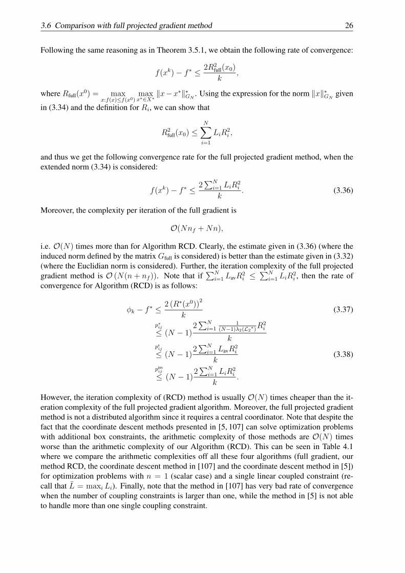
Following the same reasoning as in Theorem 3.5.1, we obtain the following rate of convergence:
f(xk)− f ∗ ≤ 2R2full(x0)
k,
where Rfull(x0) = max
x:f(x)≤f(x0)maxx∗∈X∗
∥x−x∗∥∗GN. Using the expression for the norm ∥x∥∗GN
given
in (3.34) and the definition for Ri, we can show that
R2full(x0) ≤
N∑i=1
LiR2i ,
and thus we get the following convergence rate for the full projected gradient method, when theextended norm (3.34) is considered:
f(xk)− f ∗ ≤ 2∑N
i=1 LiR2i
k. (3.36)
Moreover, the complexity per iteration of the full gradient is
O(Nnf +Nn),
i.e. O(N) times more than for Algorithm RCD. Clearly, the estimate given in (3.36) (where theinduced norm defined by the matrix Gfull is considered) is better than the estimate given in (3.32)(where the Euclidian norm is considered). Further, the iteration complexity of the full projectedgradient method is O (N(n+ nf )). Note that if
∑Ni=1 LavR
2i ≤
∑Ni=1 LiR
2i , then the rate of
convergence for Algorithm (RCD) is as follows:
ϕk − f ∗ ≤ 2 (R∗(x0))2
k(3.37)
p∗ij≤ (N − 1)
2∑N
i=11
(N−1)λ2(L2∗)R2
i
kpsij
≤ (N − 1)2∑N
i=1 LavR2i
k(3.38)
pinvij
≤ (N − 1)2∑N
i=1 LiR2i
k.
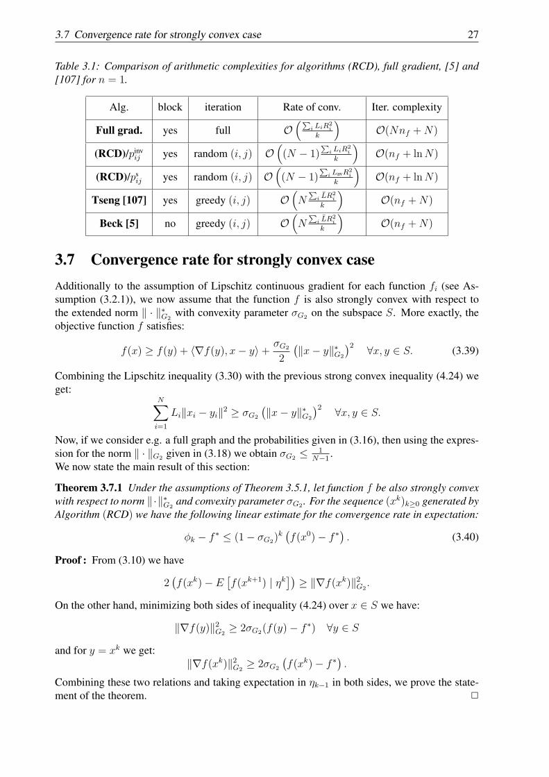
However, the iteration complexity of (RCD) method is usually O(N) times cheaper than the it-eration complexity of the full projected gradient algorithm. Moreover, the full projected gradientmethod is not a distributed algorithm since it requires a central coordinator. Note that despite thefact that the coordinate descent methods presented in [5, 107] can solve optimization problemswith additional box constraints, the arithmetic complexity of those methods are O(N) timesworse than the arithmetic complexity of our Algorithm (RCD). This can be seen in Table 4.1where we compare the arithmetic complexities off all these four algorithms (full gradient, ourmethod RCD, the coordinate descent method in [107] and the coordinate descent method in [5])for optimization problems with n = 1 (scalar case) and a single linear coupled constraint (re-call that L = maxi Li). Finally, note that the method in [107] has very bad rate of convergencewhen the number of coupling constraints is larger than one, while the method in [5] is not ableto handle more than one single coupling constraint.
3.7 Convergence rate for strongly convex case 27
Table 3.1: Comparison of arithmetic complexities for algorithms (RCD), full gradient, [5] and[107] for n = 1.
Alg. block iteration Rate of conv. Iter. complexity
Full grad. yes full O(∑
i LiR2i
k
)O(Nnf +N)
(RCD)/pinvij yes random (i, j) O
((N − 1)
∑i LiR
2i
k
)O(nf + lnN)
(RCD)/psij yes random (i, j) O
((N − 1)
∑i LavR2
i
k
)O(nf + lnN)
Tseng [107] yes greedy (i, j) O(N
∑i LR
2i
k
)O(nf +N)
Beck [5] no greedy (i, j) O(N
∑i LR
2i
k
)O(nf +N)
3.7 Convergence rate for strongly convex caseAdditionally to the assumption of Lipschitz continuous gradient for each function fi (see As-sumption (3.2.1)), we now assume that the function f is also strongly convex with respect tothe extended norm ∥ · ∥∗G2
with convexity parameter σG2 on the subspace S. More exactly, theobjective function f satisfies:
f(x) ≥ f(y) + ⟨∇f(y), x− y⟩+ σG2
2
(∥x− y∥∗G2
)2 ∀x, y ∈ S. (3.39)
Combining the Lipschitz inequality (3.30) with the previous strong convex inequality (4.24) weget:
N∑i=1
Li∥xi − yi∥2 ≥ σG2
(∥x− y∥∗G2
)2 ∀x, y ∈ S.
Now, if we consider e.g. a full graph and the probabilities given in (3.16), then using the expres-sion for the norm ∥ · ∥G2 given in (3.18) we obtain σG2 ≤ 1
N−1.
We now state the main result of this section:
Theorem 3.7.1 Under the assumptions of Theorem 3.5.1, let function f be also strongly convexwith respect to norm ∥·∥∗G2
and convexity parameter σG2 . For the sequence (xk)k≥0 generated byAlgorithm (RCD) we have the following linear estimate for the convergence rate in expectation:
ϕk − f ∗ ≤ (1− σG2)k(f(x0)− f ∗) . (3.40)
Proof : From (3.10) we have
2(f(xk)− E
[f(xk+1) | ηk
])≥ ∥∇f(xk)∥2G2
.
On the other hand, minimizing both sides of inequality (4.24) over x ∈ S we have:
∥∇f(y)∥2G2≥ 2σG2(f(y)− f ∗) ∀y ∈ S
and for y = xk we get:∥∇f(xk)∥2G2
≥ 2σG2
(f(xk)− f ∗) .
Combining these two relations and taking expectation in ηk−1 in both sides, we prove the state-ment of the theorem. 2
3.8 Convergence rate in probability 28
We notice that if fi’s are strongly convex functions with respect to the Euclidian norm, withconvexity parameter σi, i.e.
fi(xi) ≥ fi(yi) + ⟨∇fi(yi), xi − yi⟩+σi2∥xi − yi∥2 ∀xi, yi ∈ Rn, i ∈ V,
then the whole function f =∑
i fi is also strongly convex w.r.t. the extended norm induced bythe positive definite matrix diag(σ), where σ = [σ1 · · ·σN ]T , i.e.
f(x) ≥ f(y) + ⟨∇f(y), x− y⟩+ 1
2∥x− y∥2diag(σ)⊗In ∀x, y ∈ RnN .
Note that in this extended norm ∥ · ∥diag(σ)⊗In the strongly convex parameter of the function f isequal to 1. It follows immediately that the function f is also strongly convex with respect to thenorm ∥ · ∥∗G2
with the strongly convex parameter σG2 satisfying:
σG2diag(σ)−1 ≼ L2 + ζeeT ,
for some ζ ≥ 0. In conclusion we get the following LMI:
σG2IN ≼ diag(σ)1/2(L2 + ζeeT )diag(σ)1/2.
From Theorem 3.7.1 it follows that in order to get a better convergence rate we need to searchfor σG as large as possible. Therefore, for strongly convex functions the optimal probabilities arechosen as the solution of the following SDP problem:
p∗ij = arg maxζ≥0,σG2
,L∈MσG2 (3.41)
σG2IN ≼ diag(σ)1/2(L2 + ζeeT )diag(σ)1/2.
3.8 Convergence rate in probabilityIn this section we estimate the quality of random point xk, quantifying the confidence of reachingthe accuracy ϵ for the optimal value. We denote by ρ a confidence level. Then, we have thefollowing lemma:
Lemma 3.8.1 Let ξkk≥0 be a nonnegative, nonincreasing sequence of discrete random vari-ables with one of the properties:
(i) E [ξk+1|ξk] ≤ ξk −ξ2kr
for k ≥ 0 and constant r > ϵ.
(ii) E [ξk+1|ξk] ≤(1− 1
r
)ξk for k ≥ 0 and constant r > 1.
If the first part of the lemma holds and choose K such that
K ≥ r
ϵ
(1 + ln
1
ρ
)+r
ξ0+ 2
or if the second part holds and choose K satisfying
K ≥ r lnξ0ϵρ,
then we have the following probability Prob(ξK ≤ ϵ) ≥ 1− ρ.
3.8 Convergence rate in probability 29
Proof : The proof uses a similar reasoning as in Theorem 1 in [93] and is derived from theMarkov inequality. For completeness, we give the proof below. We introduce the sequence ofrandom variables ξk,ϵk:
ξk,ϵ =
ξk if ξk ≥ ϵ
0 otherwise,
and observe that ξk,ϵ ≤ ϵ if and only if ξk ≤ ϵ. Applying Markov inequality, we have:
Pr(ξk ≥ ϵ) = Pr(ξk,ϵ ≥ ϵ) ≤ E[ξk,ϵ]
ϵ.
Let us define βk = E[ξk,ϵ]. Then, the lemma is proved provided that there exists some index Ksuch that βK ≤ ϵρ. From property (i) and the definition of ξk,ϵ we have:
E[ξk+1,ϵ|ξk,ϵ
]≤ ξk,ϵ − (ξk,ϵ)2
r≤ (1− ϵ
r)ξk,ϵ ∀k ≥ 0.
Taking now the expectation we obtain:
βk+1 ≤ βk − (βk)2
r, βk+1 ≤
(1− ϵ
r
)βk ∀k ≥ 0. (3.42)
Based on the first inequality in (3.42) we get:
1
βk+1− 1
βk=βk − βk+1
βk+1βk≥ βk − βk+1
(βk)2≥ 1
r∀k ≥ 0,
and using it repeatedly we obtain 1βk ≥ 1
β0 + kr. Therefore, by choosing the index k1 ≥ r
ϵ− r
ξ0
we have βk1 ≤ ϵ. Let us now choose the index k2 ≥ rϵlog 1
ρ, then by taking K ≥ k1 + k2, the
following holds:
βK ≤ βk1+k2 ≤(1− ϵ
r
)k2βk1 ≤
((1− ϵ
r
) 1ϵ
)r log 1ρ
ϵ
≤ (exp− 1r )r log
1ρ ϵ ≤ ϵρ.
If inequality (ii) holds, using the same reasoning as before and taking K ≥ r log ξ0
ϵρwe have:
βK ≤(1− 1
r
)K
β0 ≤((
1− 1
r
)r)log ξ0
ϵρ
ξ0 ≤ ϵρ.
2
Considering now the sequence of random variable ξk = f(xk) − f ∗ in the previous lemma, wereach the following result:
Theorem 3.8.2 Under the assumptions of Theorem 3.5.1, let us choose
k ≥ R2(x0)
ϵ
(1 + ln
1
ρ− ϵ
f(x0)− f ∗
)+ 2,
3.9 Random pairs sampling 30
then the random sequence (xk)k≥0 generated by Algorithm (RCD) for solving (3.1) satisfies:
Prob(f(xk)− f ∗ ≤ ϵ) ≥ 1− ρ.
If additionally, the function f is also strongly convex with respect to norm ∥ · ∥∗G2and convexity
parameter σG2 , choosing k to satisfy:
k ≥ 1
σG2
lnf(x0)− f ∗
ϵρ
it is ensured that:Prob
(f(xk)− f ∗ ≤ ϵ
)≥ 1− ρ.
Proof : From inequality (3.20) we note that random variable ξk = f(xk)− f ∗ has the property:ξk+1 ≤ ξk −
ξ2kr
, where we assume r = R2(x0) > ϵ. Note that ξk satisfies the first conditions ofLemma 3.8.1, thus we get the first statement of the theorem.
For the second part, from Markov inequality and relation (4.26) we have:
Prob(f(xk)− f ∗ ≥ ϵ) ≤ ϕk − f ∗
ϵ≤ 1
ϵ(1− σG2)
k(f(x0)− f ∗).
Choosing k as in the statement of the theorem we have that Prob(f(xk) − f ∗ ≥ ϵ) ≤ ρ, so thatthe second statement of the theorem is now proved. 2
3.9 Random pairs samplingSince the (RCD) method is intended for problems of huge dimensions and is based on choosingat each iteration a pair of coordinates, we need a fast procedure to generate random pairs that aredistributed according to a given probability distribution. In this section we present a procedurefor generating random coordinate pairs for a given discrete probability distribution (pij)(i,j)∈E ona graph G = (V,E) with np edges:
Pr[(i, j) = (i0, j0)] = pi0j0 .
Given the discrete probability distribution with a finite number np of indices at which the prob-ability mass function takes non-zero values, i.e. pij > 0 for all (i, j) ∈ E, we propose thefollowing sampling pair algorithm. First, we construct a sequence of sorted numbers as follows:we divide the interval [0, 1) into np subintervals
[0, pi1j1), [pi1j1 , pi1j1 + pi2j2), · · · , [np−1∑ℓ=1
piℓjℓ , 1),
where we used that∑np
ℓ=1 piℓjℓ = 1. Clearly, the width of interval ℓ equals the probability piℓjℓ .Note that the preliminary computations for the subintervals consist of np − 2 additions.Let us now describe our random pair generator:
1. input: a uniformly distributed random number u
2. use the binary search algorithm to determine the index ℓu for which∑ℓu−1
ℓ=1 piℓjℓ ≤ u <∑ℓuℓ=1 piℓjℓ
3.10 Generalizations 31
3. output: the sampling pair (iℓu , jℓu).
This scheme implements correctly the random pair generator. Since the sampling algorithm de-scribed above is based on binary search [41], which halves the search interval at each iteration, ithas complexityO(ln(np)) ≤ 2 ln(N) and requires generating only one uniform random number.There also exist sampling algorithms with constant computational time, based on some precom-puted sequences, but the time required for the initialization of these sequences is O(np) (seee.g. [113]). The sampling algorithm from [76] can also be adapted to generate random pairs fora given probability distribution.
3.10 GeneralizationsIn this section we extend the main results of the previous sections to a more general randomizedblock coordinate descent algorithm and to problems with more general equality constraints.
3.10.1 Parallel coordinate descent algorithmParallel implementations of Algorithm (RCD) are possible, i.e. we can choose in parallel dif-ferent block coordinates and update x in all these components. Usually, Algorithm (RCD) canbe accelerated by parallelization, i.e. by using more than one pair per iteration usually corre-sponding to the number of available processors. In this section we extend the main results ofthe previous sections to general randomized block coordinate descent algorithm that chooses anM -tuple of indices. The (RCD)(i,j) algorithm can be extended to update more than two pairs(i, j) at each iteration. For example, taking a positive integer M ≤ N , we denote with N anysubset of V having cardinality M . Here, we do not assume explicitly additional structure suchas those imposed by a graph, i.e. we consider all to all communication. Then, we can derivea randomized M block coordinate descent algorithm where we update at each iteration only Mblocks in the vector x. Let us define N = (i1, · · · iM) with il ∈ V , sN = [si1 · · · siM ]T ∈ RMn
and LN = [Li1 · · ·LiM ]T ∈ RM . Under assumption (3.2) the following inequality holds:
f(x+∑i∈N
Uisi) ≤ f(x) + ⟨∇fN (x), sN ⟩+1
2∥sN∥2diag(LN ). (3.43)
Based on the inequality (4.29) we can define a general randomized M block coordinate descentalgorithm, let us call it (RCD)M . Given an x in the feasible set S, we choose the coordinateM -tuple N with probability pN . Let the next iterate be chosen as follows:
x+ = x+∑i∈N
Uidi,
i.e. we update M components in the vector x, where the direction dN is determined by requiringthat the next iterate x+ to be also feasible and minimizing the right hand side in (4.29), i.e.:
dN = arg minsN :
∑i∈N si=0
f(x) + ⟨∇fN (x), sN ⟩+1
2∥sN∥2diag(LN )
or explicitly
di =1
Li
∑j∈N
1Lj
(∇fj(xj)−∇fi(xi))∑j∈N
1Lj
∀i ∈ N .
In conclusion, we obtain the following randomized M -block coordinate descent method:
3.10 Generalizations 32
Algorithm (RCD)M : Random M -Block Coordinate Descent Method
1. choose the M -tuple Nk = (i1k, · · · iMk ) with probability pN2. set xk+1
i = xki ∀i /∈ Nk and xk+1i = xki + dki ∀i ∈ Nk.
Based on the inequality (4.29) the following decrease in objective function can be derived:
f(x+) ≤ f(x)−∑i∈N
1
2Li
∥∑
j∈N1Lj
(∇fj(xj)−∇fi(xi)) ∥2
(∑
j∈N1Lj)2
= f(x)− 1
2∇f(x)TGN∇f(x),
where GN is defined as
GN =
[diag(L−1
N )− 1∑i∈N 1/Li
L−1N (L−1
N )T]⊗ In,
where we redefine LN ∈ RN as the vector with components zero outside the index set N andcomponents Li for i ∈ N . Therefore, taking the expectation over the random M -tuple N ⊂ V ,we obtain the following inequality:
E[f(x+) | η] ≤ f(x)− 1
2∇f(x)TGM∇f(x). (3.44)
The corresponding matrix GM =∑
N pNGN = LM ⊗ In is still positive semidefinite andhas an eigenvalue λ1(GM) = 0. Based on the decrease in expectation (4.30), a similar rate ofconvergence will be obtained for this general algorithm (RCD)M as in the previous sections, butdepending on M . For example, we can consider probabilities of the form:
pinvN =
∑i∈N 1/Li∑
N∑
i∈N 1/Li
.
We can see that:
Σ−1M =
∑N
∑i∈N
1/Li =
(MN)∑j=1
∑i∈Nj
1/Li =
(MN)∑j=1
N∑i=1
1i,Nj1/Li
=N∑i=1
1/Li
(MN)∑j=1
1i,Nj
=N∑i=1
1/Li
(M − 1
N − 1
).

3.10 Generalizations 33
Using a similar reasoning we can derive that:
LM =1
Σ−1M
∑N
[(∑i∈N
1/Li)diag(L−1N )− L−1
N (L−1N )T
]
=1
Σ−1M
(MN)∑j=1
(∑i∈Nj
1/Li)diag(L−1Nj)− L−1
Nj(L−1
Nj)T
=
1
Σ−1M
(M − 2
N − 2
)[(
N∑i=1
1/Li)diag(L−1)− L−1(L−1)T
]
=M − 1
N − 1
[diag(L−1)− 1∑N
i=1 1/Li
L−1(L−1)T
].
In conclusion, for this choice of the probabilities we get the following convergence rate forAlgorithm (RCD)M in the expected values of the objective function:
ϕk − f ∗ ≤ N − 1
M − 1· 2∑
i LiR2i
k.
Note that for M = 2 we obtain the convergence rate in (3.22) for 2-block coordinate descentalgorithm (RCD) based on probabilities pinv
ij , while for M = N we recover the convergence rateof full gradient. We clearly see that the theoretical speedup, as compared to the 2-block case, isa simple expression depending linearly on the number M of parallel processors.
3.10.2 Optimization problems with general equality constraintsWe now consider optimization problems with general linear equality constraints:
f ∗ = minx∈Rnf(x) : s.t. Ax = 0, (3.45)
where A ∈ Rm×n. We show in this section that the random coordinate descent algorithm (RCD)can be generalized to solve problem (3.45). Using a similar reasoning as in previous sections, fora given feasible x for problem (3.45) we derive our next feasible iterate x+ = x + Uidi + Ujdjby solving an optimization subproblem with the constraints Aisi+Ajsj = 0, whose solution canbe computed explicitly:
[dTi dTj ]T =− 1
Lij
(∇ijf(x)− Aij(A
TijAij)
−1ATij∇ijf(x)
),
provided that the matrix ATij = [Ai Aj] ∈ Rm×ni+nj has full row rank. We also use the compact
notation ∇ijf = [∇fTi ∇fT
j ]T . In case that AT
ij is zero then, [di dj]T = − 1Lij∇ijf(x). In
conclusion, in the following we assume that:The matrix AT
ij is either full row rank or zero for any (i, j) ∈ E, each row in the matrix A is non-zero and m < n and we have available a probability distribution (pij)(i,j)∈E over the connectedgraph G.
We can prove a similar decrease in the objective function as before and we can define thematrixGij ∈ Rn×n containing the block matrix Ini+nj
−Aij(ATijAij)
−1ATij in the entries given by
the indexes i and j and zero in the rest of the blocks. It is straightforward to see that GijAT = 0,
3.11 Applications 34
i.e. each row in the matrix A is an eigenvector of Gij associated to the zero eigenvalue. We cansimilarly define the matrix G =
∑(i,j)∈E
pijLi+Lj
Gij that will have the rows of A as eigenvectorsassociated to the zero eigenvalue, since GAT = 0. The same rate of convergence can be provedin this general linear constraint case as in the previous sections. Note that in this general linearconstraints case we need to invert at each iteration of the randomized block coordinate descentalgorithm a matrix AT
ijAij ∈ Rm×m. As long as m is small or these matrices are easy to invertwe can still use the algorithm to solve distributively the general linear constraint problem (3.45).For example, if all the matrices Ai are diagonal, then each iteration of the algorithm can beimplemented efficiently.
3.11 ApplicationsProblem (3.1) arises in many real applications, e.g. resource allocation in economic systems [34]or distributed computer systems [45], in distributed control [65], in traffic equilibrium problemsor network flow [8] and other areas. For example, we can interpret it as N agents exchangingn goods to minimize a total cost, where the constraint
∑i xi = 0 is the equilibrium or market
clearing constraint. In this context [xi]j ≥ 0 means that agent i receives [xi]j of good j fromexchange and [xi]j < 0 means that agent i contributes |(xi)j| of good j to exchange.Problem (3.1) can also be seen as the dual problem corresponding to an optimization of a sumof convex functions. Consider the following convex optimization problem that arises in manyengineering applications such as signal processing, distributed control and network flow [8, 21,24, 30, 65, 74, 110]:
g∗ = minv∈∩N
i=1Qi
g1(v) + · · ·+ gN(v), (3.46)
where gi are all convex functions and Qi are convex sets. This problem can be reformulated as:
minui∈Qi,ui=v ∀i∈V
g1(u1) + · · ·+ gN(uN).
Let us define u = [uT1 · · ·uTN ]T and g(u) = g1(u1)+· · ·+gN(uN). By duality, using the Lagrangemultipliers xi for the constraints ui = v, we obtain the separable convex problem (3.1), wherefi(xi) = g∗i (xi) and g∗i is the convex conjugate of the function gi = gi + 1Qi
, i.e.
fi(xi) = maxui∈Qi
⟨xi, ui⟩ − gi(ui) ∀i. (3.47)
Further we have f ∗ + g∗ = 0. Note that if gi is strongly convex, then the convex conjugate fi iswell-defined and has Lipschitz continuous gradient, so that Assumption 3.2.1 holds. A particularapplication is the problem of finding the projection of a point v0 in the intersection of the convexsets ∩N
i=1Qi. This problem can be written as an optimization problem in the form:
minv∈∩N
i=1Qi
p1∥v − v0∥2 + · · ·+ pN∥v − v0∥2,
where pi > 0 such that∑
i pi = 1. This is a particular case of the separable problem (3.46).Note that since the functions gi(v) = pi∥v − v0∥2 are strongly convex, then fi have Lipschitzcontinuous gradient with Lipsctiz constants Li = 1/pi for all i. We can also consider the problemof finding a point in the intersection of some convex sets:
minv∈∩N
i=1Qi
cT1 v + · · ·+ cTNv, (3.48)
3.11 Applications 35
which again applying duality as above, it will lead to the separable convex problem (3.1). Sincein this case the objective functions gi(v) = cTi v are linear, it follows that the functions fi arenot smooth anymore (i.e. Assumption 3.2.1 will not hold in this case) and smoothing techniquesneed to be applied. In this scenario we can consider smoothing (3.48) as follows:
minv∈∩N
i=1Qi
(cT1 v + pi∥v∥2) + · · ·+ (cTNv + pN∥v∥2).
3.11.1 Recovering approximate primal solutions from full dual gradientFrom Section 3.6 we have obtain the following convergence rate for the full projected gradientmethod:
f(xk)− f ∗ ≤ 2∑
i LiR2i
k∀k > 0.
Let us define the primal iterates:
uki = arg minui∈Qi
gi(ui)− ⟨xki , ui⟩ ∀i ∈ V.
It follows immediately from (3.47) that ∇fi(xki ) = uki and fi(xki ) + gi(uki ) = ⟨xki , uki ⟩ for all
i ∈ V and k ≥ 0. Then, we also get: ⟨∇f(xk), xk⟩ = ⟨uk, xk⟩ = f(xk) + g(uk) for all k ≥ 0.We also want to provide estimates on the convergence rate of the primal sequence ukk≥0. Letus apply 2k iterations of the full projected gradient method. From the previous discussion wehave that the following inequality holds (see (3.33)):
f(xl+1) ≤ f(xl)− 1
2∥∇f(xl)∥2GN
∀l = k, · · · , 2k − 1.
Adding these inequalities for l = k, · · · , 2k − 1 we obtain:
f(xk)− f(x2k) ≥ 1
2
2k−1∑l=k
∥∇f(xl)∥2GN≥ k
2∥∇f(xk∗)∥2GN
,
wherek∗ = arg min
l=k,··· ,2k−1∥∇f(xl)∥2GN
.
Taking into account that after k steps we have sublinear convergence in the form O(2∑
i LiR2i
k),
we get:
∥∇f(xk∗)∥2GN≤ 2(f(xk)− f(x2k))
k≤ 2(f(xk)− f ∗)
k≤ 4
∑i LiR
2i
k2
f(xk∗)− f ∗ ≤ f(xk)− f ∗ −
k∗−1∑l=k
1
2∥∇f(xl)∥2GN
≤ 2∑
i LiR2i
k.
Further, since ∇fi(xki ) = uki we have that:
∥∇f(xk∗)∥2GN
(3.33)=
N∑i=1
1
2Li
∥∥∥∥∥∇fi(xk∗i )−∑N
j=11Lj∇fj(xk
∗j )∑N
j=11Lj
∥∥∥∥∥2
=N∑i=1
1
2Li
∥∥∥∥∥uk∗i −∑N
j=11Ljuk
∗j∑N
j=11Lj
∥∥∥∥∥2
.
3.11 Applications 36
Now, if we define vk∗ =
∑Nj=1
1Lj
uk∗j∑N
j=11Lj
, then the full projected gradient method produces after 2k
iterations the dual variables xk∗ with∑
i xk∗i = 0 and primal variables uk∗i ∈ Qi for all i ∈ V
such that with their convex combination vk∗ satisfies the following dual suboptimality:
f(xk∗)− f ∗ ≤ 2
∑Ni=1 LiR
2i
k. (3.49)
and primal feasibility violation:
uk∗
j ∈ Qj and ∥uk∗j − vk∗∥2 ≤ 8Lj(
∑Ni=1 LiR
2i )
k2∀j ∈ V, (3.50)
i.e. dist(vk∗ , Qj) ≤ O(1/k) for all j ∈ V . We further require that the collection of sets Qj , withj = 1, . . . , N , possesses a linear regularity property [4, Definition 5.6, page 40], i.e. there existsa positive scalar θ such that
∥v − Π∩jQj(v)∥ ≤ θmax
j∥v − ΠQj
(v)∥ ∀v.
This property is automatically satisfied when Qj are polyhedral sets. The discussions in [25]identify several other situations where the linear regularity condition holds, and indicates thatthis condition is a mild restriction in practice. Under this requirement we also have that:
dist(vk∗,∩jQj) ≤ γmax
jdist(vk
∗, Qj)
for some constant γ > 0. Therefore, under the notion of linear regularity we also get thatdist(vk∗ ,∩jQj) ≤ O(1/k).
Chapter 4
Random coordinate descent methods forsingly linearly constrained smoothoptimization
In this chapter we develop randomized block-coordinate descent methods for minimizing multi-agent convex optimization problems with a single linear coupled constraint over networks andprove that they obtain in expectation an ϵ accurate solution in at mostO( 1
λ2(Q)ϵ) iterations, where
λ2(Q) is the second smallest eigenvalue of a matrix Q that is defined in terms of the probabilitiesand the number of blocks. Due to the coupling in the constraints we introduce a 2-block variantof random coordinate descent method, that involves at each iteration the closed form solutionof an optimization problem only with respect to two block variables while keeping all the othervariables fixed. However, the computational complexity per iteration of our methods is muchsimpler than the one of a method based on full gradient information and each iteration can becomputed in a completely distributed way. We focus on how to choose the probabilities to makethese randomized algorithms to converge as fast as possible and we arrive at solving a sparseSDP. Analysis for rate of convergence in probability is also provided. For strongly convex func-tions our distributed algorithms converge linearly. We also extend the main algorithm to a moregeneral random coordinate descent method and to problems with more general linearly coupledconstraints. Preliminary numerical tests confirm that on very large optimization problems ourmethod is much more numerically efficient than methods based on full gradient. This chapter isbased on paper [58, 59, 69].
4.1 IntroductionMany of today’s problems can be addressed within the framework of networked systems, that arecomplex and large in dimension, whose structure may be hierarchical, multistage or dynamicaland they have multiple decision-makers. Systems that are very large can be broken down intosmaller, more malleable subsystems called decompositions and these mathematical models mayrepresent the viewpoints of different decision-makers or may display emphasis on any one ormore of the various aspects of the system. How to think about relationships between thesevarious decompositions has led to much of the recent work within the general subject of thestudy of large-scale networked systems.The goal of this chapter is to develop efficient (block) coordinate descent type algorithmsfor solving coupled linear constrained optimization problems that appear in the context of
37
4.1 Introduction 38
networked systems (e.g. distributed control, network utility maximization, resource alloca-tion, DSL dynamic spectrum management and multistage stochastic convex programming)[110, 117, 121, 126]. With each subsystem in the network is associated a local variable so thattogether they are coupled via a set of linear equalities and we need to minimize a smooth convexobjective function.For a centralized setup and problems of moderate size there exist many iterative algorithms suchas Newton, quasi-Newton or projected gradient methods. The design of decentralized algorithmsfor such problems was investigated for the first time in [31, 34]. But the methods proposed inthese papers are not fully distributed since they usually require a central coordinator. In [32,121] distributed weighted gradient methods were proposed to solve resource allocation problems(called center-free algorithms since they do not require a central coordinating entity). However,the problems that we consider in this chapter have dimension of the optimization variables verylarge so that usual methods based on whole gradient computations are prohibitive. A recentdevelopment in the area of large-scale optimization is the coordinate descent framework. Thesemethods were among the first optimization methods studied in literature [8] but until recently theyhaven’t received much attention. For recent application we name just few of them: support vectormachine [17, 109, 124], compressed sensing [47], protein loop closure [15] and optimization[53, 89, 108, 120, 125].In this chapter we develop random coordinate descent methods suited for large scale problemswhere the information cannot be gathered centrally, but rather the information is distributed overall the nodes of the network, which may not be equally responsive, so that at a given time it isnecessary to work with whatever data is available then. Moreover, we focus on coupled linearconstrained optimization problems (i.e. the constraint set is coupled). Due to the coupling in theconstraints we introduce a 2-block variant of random coordinate descent method, that involves ateach iteration the closed form solution of an optimization problem only with respect to two blockvariables while keeping all the other variables fixed. We prove for our main distributed algorithma convergence rate in expectation of order O( 1
λ2(Q)k), where λ2(Q) is the second smallest eigen-
value of a matrix Q that depends on the the choice of the probabilities and the number of blocks.We focus on how to design the probabilities to make this distributed algorithm converge as fastas possible and we prove that this problem can be recast as a sparse SDP.We show that for functions with cheap coordinate derivatives the proposed algorithms are muchfaster, either in worst case complexity analysis or numerical implementation, than schemes basedon full gradient information. But our methods also offers other important advantages, e.g. dueto the randomization our algorithms are easier to analyze, they lead to more robust output andare adequate for modern computational architectures (e.g distributed and parallel architectures).Analysis for rate of convergence in probability is also provided. For strongly convex functionswe prove that they converge linearly. Note that the algorithms presented in this chapter are ageneralization of the algorithm from previous chapter to more general optimization models andalso the convergence rate analysis derived here is based on different tools than the ones fromChapter 3.The chapter is organized as follows. In Section 4.2 the problem formulation, assumptions andnotations used in the chapter are presented. In Section 4.3, we derive a randomized block coor-dinate descent method and analyze the rate of convergence in expectation. Then, we deal withthe design of the optimal probabilities that makes the new algorithm converge as fast as possible.We also show that the problems we consider in this chapter can be solved with an arbitrarilyhigh confidence level in Section 4.6. In Section 4.7 we prove linear convergence for the stronglyconvex case. In Section 4.8 we extend the main results of the previous sections to a more generalrandom coordinate descent algorithm and to problems with more general local norms. Finally,
4.2 Problem formulation 39
in Section 4.9 we present preliminary numerical results that show the efficiency of our algorithmon very large optimization problems.
4.2 Problem formulationWe work in the space Rn composed by column vectors. For x, y ∈ Rn denote the standard Eu-clidean inner product ⟨x, y⟩ =
∑ni=1 xiyi and the Euclidean norm ∥x∥ = (
∑ni=1 x
2i )
1/2. We usethe same notation ⟨·, ·⟩ and ∥ · ∥ for spaces of different dimension. For convenience, sometimeswe also use xTy =
∑ni=1 xiyi (especially when we work with matrices). In this chapter we
develop a random coordinate descent method for singly linear constrained convex minimizationproblems of the following form:
f ∗ = minx∈Rnf(x) : s.t. ⟨a, x⟩ = 0, (4.1)
where the objective function f is smooth and convex, and a ∈ Rn. For our problem (4.1) weassociate a network composed of several nodes V = 1, · · · , N (e.g. subsystems, sensors,web sites, etc) that can exchange information according to a communication graph G = (V,E),where E denotes the set of edges, i.e. (i, j) ∈ E ⊆ V × V models that node j sends informationto node i. We assume that graph G is undirected and connected. The local information structureimposed by graph G should be considered as part of the problem formulation.We denote the feasible set of problem (4.1) by:
S = x ∈ Rn| ⟨a, x⟩ = 0.
Let us consider a decomposition of the dimension of the variables: n =∑N
i=1 ni. We divide theidentity matrix into:
In =[U1 · · · UN
], Ui ∈ Rn×ni , i ∈ V
and use the following notation for the partial gradient: ∇if(x) = UTi ∇f(x). Moreover, for any
x =[xT1 · · · xTN
]T ∈ Rn we can write: x =∑N
i=1 Uixi, where xi ∈ Rni for all i ∈ V and we
also use xij ∈ Rni+nj to denote the vector xij =
[xi
xj
]for any pair (i, j) ∈ E. For a symmetric
matrix Q ∈ Rn×n we consider the following order of its eigenvalues: λ1 ≤ λ2 ≤ · · · ≤ λn.We also denote the set of optimal solutions of (4.1) with X∗. We notice that the KKT conditionsof problem (1) are given by the following: x∗ =
[(x∗1)
T · · · (x∗N)T]T is an optimal point for
convex problem (1) if and only if
⟨a, x∗⟩ = 0, ∇f(x∗) = λ∗a, for some scalar λ∗ ∈ R. (4.2)
Singly linear constrained optimization problems (4.1) arise in many areas such as resource al-location in economic systems [34] or distributed computer systems [45], network utility max-imization [117], DSL dynamic spectrum management [110] and multistage stochastic convexprogramming [126]. Control theory on one hand, and economics, management and computerscience on the other, have paid considerable attention to mathematical models of resource al-location within the context of a hierarchical decentralized organization. There are two mainclasses of decentralized mechanisms for resource allocation: price directed [34] and resource-directed [31]. However, most of the methods are not fully distributed because they either require

4.3 Random block coordinate descent method 40
a central price coordinator or a central resource dispatcher. In [32,121] distributed weighted gra-dient methods were proposed and studied to solve a similar problem as in (4.1). In particular, theauthors in [121] consider a strongly convex function f with a positive definite Hessian. Note thatthese papers propose a class of center-free algorithms (the term center-free refers to the absenceof a supervisor) with the following iteration: for all i ∈ V and k ≥ 0 update
xk+1i = xki −
∑j∈Ni
wij
(∇jf(x
k)−∇if(xk)), (4.3)
where Ni denotes the set of neighbors of node i in the graph G and the full gradient needs to becomputed. Throughout the chapter the superscript k denotes the iteration counter of an algorithmand the subscript i denotes the ith (block) component of a vector. Under the strong convexityassumption of f and provided that the weights wij are designed using local information or bysolving an SDP, but satisfying certain relations, a linear rate of convergence is obtained.We now state the main assumption of this chapter:
Assumption 4.2.1 We assume that function f has component-wise Lipschitz continuous gradientwith constants Li, i.e. there exist scalars Li > 0 such that:
∥∇if(x+ Uisi)−∇if(x)∥ ≤ Li∥si∥ ∀x∈Rn, si∈Rni , i∈V.
By standard reasoning, it can be proved that [75]:
f(x+ Uisi) ≤ f(x) + ⟨∇if(x), si⟩+Li
2∥si∥2 (4.4)
for all x ∈ Rn, si ∈ Rni and i ∈ V .
4.3 Random block coordinate descent methodIn this section we present a randomized coordinate descent algorithm for solving problem (4.1),with very cheap numerical complexity per iteration and where only neighboring agents are re-quired to communicate with each other. At a certain iteration, having a feasible estimate x of theoptimizer, we choose randomly a pair (i, j) ∈ E with probability pij > 0 (if (i, j) ∈ E, thenpij = 0). Since we assume an undirected graph, we consider pij = pji (the generalization of thescheme to directed graphs is straightforward, provided that we consider the symmetric versionof the matrices that will be defined in the sequel). We define the random variable comprising thewhole history of previous events as:
ωk = (i0, j0), . . . , (ik, jk).
We first show that if the function f has component-wise Lipschitz continuous gradient, then fhas Lipschitz continuous gradient in each pair (i, j).
Lemma 4.3.1 Let f : Rn → R be a smooth convex function satisfying Assumption 5.4. Then,for each pair (i, j) with i = j, denoting Lij = Li + Lj , we have:∥∥∥∥∥
[∇if(x+ Uisi + Ujsj)−∇if(x)
∇jf(x+ Uisi + Ujsj)−∇jf(x)
]∥∥∥∥∥ ≤ Lij
∥∥∥∥∥[si
sj
]∥∥∥∥∥for all x ∈ Rn, si ∈ Rni and sj ∈ Rnj .
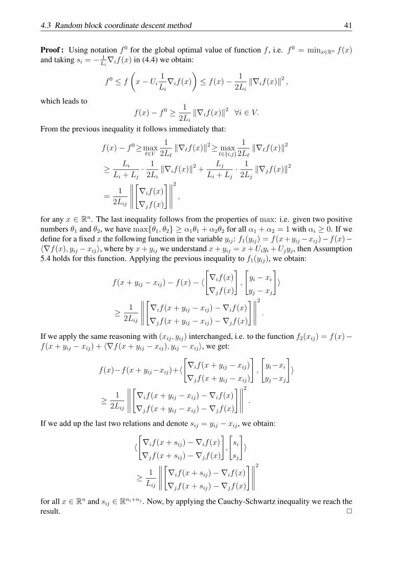
4.3 Random block coordinate descent method 41
Proof : Using notation f 0 for the global optimal value of function f , i.e. f 0 = minx∈Rn f(x)and taking si = − 1
Li∇if(x) in (4.4) we obtain:
f 0 ≤ f
(x− Ui
1
Li
∇if(x)
)≤ f(x)− 1
2Li
∥∇if(x)∥2 ,
which leads tof(x)− f 0 ≥ 1
2Li
∥∇if(x)∥2 ∀i ∈ V.
From the previous inequality it follows immediately that:
f(x)− f 0≥maxℓ∈V
1
2Lℓ
∥∇ℓf(x)∥2≥ maxℓ∈i,j
1
2Lℓ
∥∇ℓf(x)∥2
≥ Li
Li + Lj
· 1
2Li
∥∇if(x)∥2 +Lj
Li + Lj
· 1
2Lj
∥∇jf(x)∥2
=1
2Lij
∥∥∥∥∥[∇if(x)
∇jf(x)
]∥∥∥∥∥2
,
for any x ∈ Rn. The last inequality follows from the properties of max: i.e. given two positivenumbers θ1 and θ2, we have maxθ1, θ2 ≥ α1θ1 + α2θ2 for all α1 + α2 = 1 with αi ≥ 0. If wedefine for a fixed x the following function in the variable yij: f1(yij) = f(x+yij−xij)−f(x)−⟨∇f(x), yij − xij⟩, where by x+ yij we understand x+ yij = x+Uiyi +Ujyj , then Assumption5.4 holds for this function. Applying the previous inequality to f1(yij), we obtain:
f(x+ yij − xij)− f(x)− ⟨
[∇if(x)
∇jf(x)
],
[yi − xiyj − xj
]⟩
≥ 1
2Lij
∥∥∥∥∥[∇if(x+ yij − xij)−∇if(x)
∇jf(x+ yij − xij)−∇jf(x)
]∥∥∥∥∥2
.
If we apply the same reasoning with (xij, yij) interchanged, i.e. to the function f2(xij) = f(x)−f(x+ yij − xij) + ⟨∇f(x+ yij − xij), yij − xij⟩, we get:
f(x)−f(x+ yij−xij)+⟨
[∇if(x+ yij − xij)∇jf(x+ yij − xij)
],
[yi−xiyj−xj
]⟩
≥ 1
2Lij
∥∥∥∥∥[∇if(x+ yij − xij)−∇if(x)
∇jf(x+ yij − xij)−∇jf(x)
]∥∥∥∥∥2
.
If we add up the last two relations and denote sij = yij − xij , we obtain:
⟨
[∇if(x+ sij)−∇if(x)
∇jf(x+ sij)−∇jf(x)
],
[si
sj
]⟩
≥ 1
Lij
∥∥∥∥∥[∇if(x+ sij)−∇if(x)
∇jf(x+ sij)−∇jf(x)
]∥∥∥∥∥2
for all x ∈ Rn and sij ∈ Rni+nj . Now, by applying the Cauchy-Schwartz inequality we reach theresult. 2
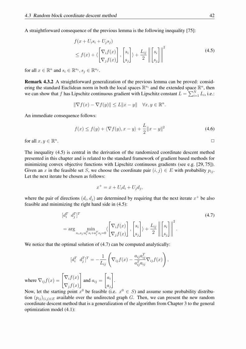
4.3 Random block coordinate descent method 42
A straightforward consequence of the previous lemma is the following inequality [75]:
f(x+ Uisi + Ujsj)
≤ f(x) + ⟨
[∇if(x)
∇jf(x)
],
[si
sj
]⟩+ Lij
2
∥∥∥∥∥[si
sj
]∥∥∥∥∥2
(4.5)
for all x ∈ Rn and si ∈ Rni , sj ∈ Rnj .
Remark 4.3.2 A straightforward generalization of the previous lemma can be proved: consid-ering the standard Euclidean norm in both the local spaces Rni and the extended space Rn, thenwe can show that f has Lipschitz continuous gradient with Lipschitz constant L =
∑Ni=1 Li, i.e.:
∥∇f(x)−∇f(y)∥ ≤ L∥x− y∥ ∀x, y ∈ Rn.
An immediate consequence follows:
f(x) ≤ f(y) + ⟨∇f(y), x− y⟩+ L
2∥x− y∥2 (4.6)
for all x, y ∈ Rn. 2
The inequality (4.5) is central in the derivation of the randomized coordinate descent methodpresented in this chapter and is related to the standard framework of gradient based methods forminimizing convex objective functions with Lipschitz continuous gradients (see e.g. [29, 75]).Given an x in the feasible set S, we choose the coordinate pair (i, j) ∈ E with probability pij .Let the next iterate be chosen as follows:
x+ = x+ Uidi + Ujdj,
where the pair of directions (di, dj) are determined by requiring that the next iterate x+ be alsofeasible and minimizing the right hand side in (4.5):
[dTi dTj ]T (4.7)
= arg minsi,sj :aTi si+aTj sj=0
⟨
[∇if(x)
∇jf(x)
],
[si
sj
]⟩+ Lij
2
∥∥∥∥∥[si
sj
]∥∥∥∥∥2
.
We notice that the optimal solution of (4.7) can be computed analytically:
[dTi dTj ]T = − 1
Lij
(∇ijf(x)−
aijaTij
aTijaij∇ijf(x)
),
where∇ijf(x) =
[∇if(x)
∇jf(x)
]and aij =
[ai
aj
].
Now, let the starting point x0 be feasible (i.e. x0 ∈ S) and assume some probability distribu-tion (pij)(i,j)∈E available over the undirected graph G. Then, we can present the new randomcoordinate descent method that is a generalization of the algorithm from Chapter 3 to the generaloptimization model (4.1):
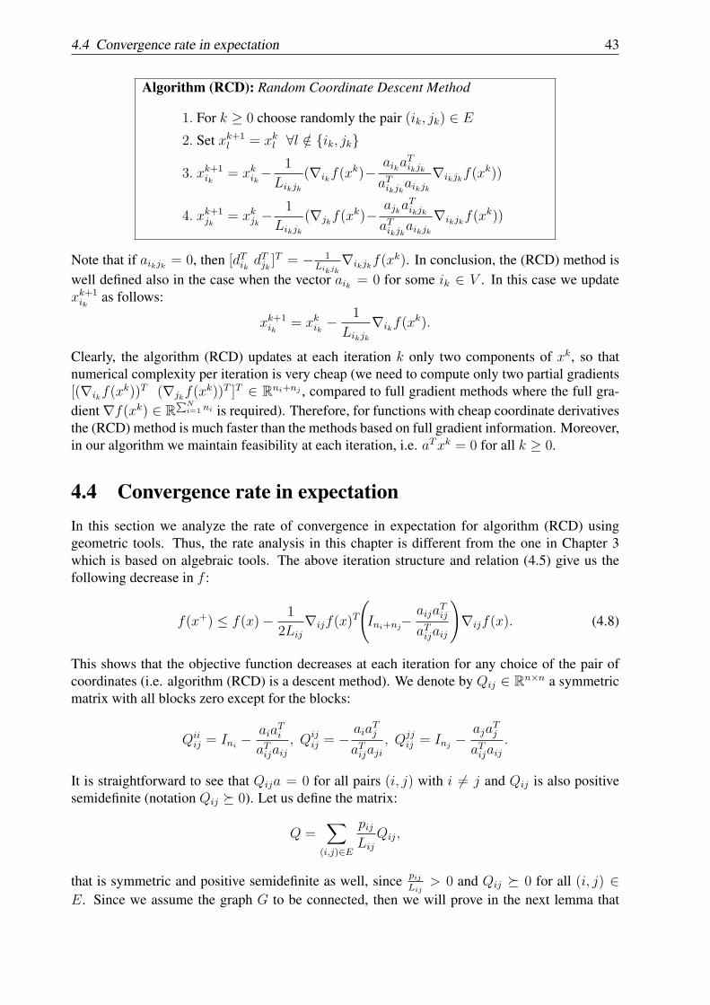
4.4 Convergence rate in expectation 43
Algorithm (RCD): Random Coordinate Descent Method
1. For k ≥ 0 choose randomly the pair (ik, jk) ∈ E2. Set xk+1
l = xkl ∀l /∈ ik, jk
3. xk+1ik
= xkik−1
Likjk
(∇ikf(xk)−
aikaTikjk
aTikjkaikjk∇ikjkf(x
k))
4. xk+1jk
= xkjk−1
Likjk
(∇jkf(xk)−
ajkaTikjk
aTikjkaikjk∇ikjkf(x
k))
Note that if aikjk = 0, then [dTik dTjk]T = − 1
Likjk∇ikjkf(x
k). In conclusion, the (RCD) method iswell defined also in the case when the vector aik = 0 for some ik ∈ V . In this case we updatexk+1ik
as follows:
xk+1ik
= xkik −1
Likjk
∇ikf(xk).
Clearly, the algorithm (RCD) updates at each iteration k only two components of xk, so thatnumerical complexity per iteration is very cheap (we need to compute only two partial gradients[(∇ikf(x
k))T (∇jkf(xk))T ]T ∈ Rni+nj , compared to full gradient methods where the full gra-
dient∇f(xk) ∈ R∑N
i=1 ni is required). Therefore, for functions with cheap coordinate derivativesthe (RCD) method is much faster than the methods based on full gradient information. Moreover,in our algorithm we maintain feasibility at each iteration, i.e. aTxk = 0 for all k ≥ 0.
4.4 Convergence rate in expectationIn this section we analyze the rate of convergence in expectation for algorithm (RCD) usinggeometric tools. Thus, the rate analysis in this chapter is different from the one in Chapter 3which is based on algebraic tools. The above iteration structure and relation (4.5) give us thefollowing decrease in f :
f(x+) ≤ f(x)− 1
2Lij
∇ijf(x)T
(Ini+nj
−aija
Tij
aTijaij
)∇ijf(x). (4.8)
This shows that the objective function decreases at each iteration for any choice of the pair ofcoordinates (i.e. algorithm (RCD) is a descent method). We denote by Qij ∈ Rn×n a symmetricmatrix with all blocks zero except for the blocks:
Qiiij = Ini
− aiaTi
aTijaij, Qij
ij = −aia
Tj
aTijaji, Qjj
ij = Inj−aja
Tj
aTijaij.
It is straightforward to see that Qija = 0 for all pairs (i, j) with i = j and Qij is also positivesemidefinite (notation Qij ≽ 0). Let us define the matrix:
Q =∑
(i,j)∈E
pijLij
Qij,
that is symmetric and positive semidefinite as well, since pijLij
> 0 and Qij ≽ 0 for all (i, j) ∈E. Since we assume the graph G to be connected, then we will prove in the next lemma that
4.4 Convergence rate in expectation 44
the matrix Q has an eigenvalue λ1(Q) = 0 (which is a simple eigenvalue) with the associatedeigenvector a. It follows that λ2(Q) > 0. This lemma is a generalization of the classical resulton Laplacian matrices to the block case with general block matrix weights. A similar result, butwith a different proof and for the scalar case can be found in [28].
Lemma 4.4.1 The multiplicity of the eigenvalue λ1(Q) = 0 is equal to the number of connectedcomponents of the graph G provided that the block entries in the vector a corresponding to eachconnected component is nonzero. In particular, if the graph G is connected, then λ2(Q) > 0.
Proof : Since Qija = 0 for all (i, j) ∈ E, then from the definition of Q we also get that Qa = 0,i.e. the matrix Q has an eigenvalue λ1(Q) = 0 with an associated eigenvector a. Since thematrix Q is symmetric, then the algebraic multiplicity of the eigenvalue λ1(Q) = 0 coincideswith the geometric multiplicity. Therefore, if λ1(Q) has multiplicity d, then there exist d linearindependent eigenvectors associated to this eigenvalue. Let v be an eigenvector corresponding toλ1(Q) = 0. Then, after some straightforward computations we derive the following sequence ofequalities:
0 = vTQv =∑
(i,j)∈E
pijLij
vTQijv
=∑
(i,j)∈E
pijLij∥aij∥2
[(aTi ai + aTj aj)(vTi vi + vTj vj)
− (vTi aiaTi vi + 2vTi aia
Tj vj + vTj aja
Tj vj)]
=∑
(i,j)∈E
pijLij∥aij∥2
[∥aij∥2∥vij∥2 − (⟨aij, vij⟩)2
],
where we recall that vij =
[vi
vj
]. Based on the Cauchy-Schwartz inequality, i.e. |⟨aij, vij⟩)| ≤
∥aij∥∥vij∥, we conclude that each term in the sum above is nonnegative and since the sum iszero, then each term must also be zero, i.e.:
|⟨aij, vij⟩)| = ∥aij∥∥vij∥ ∀(i, j) ∈ E.
However, the Cauchy-Schwartz inequality holds with equality if and only if there exist someconstants αij ∈ R such that:
vij = αijaij ∀(i, j) ∈ E.
Now, starting with any node i and applying vij = αijaij repeatedly (i.e. vi = αijai andvj = αijaj), one can see that any node l reachable from i also satisfies vl = αijal. In otherwords, there exists some scalar α = 0, such that the eigenvector v is αa on each connectedcomponent of G and is nonzero according to the hypothesis of the lemma. If there are exactly dconnected components, there are exactly d independent eigenvectors, since choosing d nonzeroconstants α1, · · · , αd (one for each connected component) determines each eigenvector uniquely.In particular, if the graph is connected, then λ1(Q) = 0 is simple and thus λ2(Q) > 0. 2
Taking the expectation in (4.8) over the random pair (i, j) we get the following decrease:
Eij[f(x+)] ≤ f(x)− 1
2∇f(x)TQ∇f(x). (4.9)
4.4 Convergence rate in expectation 45
We now introduce the following distance:
R(x0) = maxx:f(x)≤f(x0)
maxx∗∈X∗
∥x− x∗∥,
which measures the size of the level set of f given by x0. We assume that this distance is finitefor the initial iterate x0. From (4.8) it follows that algorithm (RCD) is a descent method, thusf(xk) ≤ f(x0) for all k ≥ 0. Then, the following bound holds:
∥xk − x∗∥ ≤ R(x0) ∀k ≥ 0, x∗ ∈ X∗. (4.10)
Moreover, for a given vector z ∈ Rn, we denote with z⊥ the projection of the vector z onto thesubspace S that is orthogonal to the vector a. It follows immediately that z⊥ can be computedexplicitly in our case:
z⊥ = (In −aaT
aTa)z.
Using the notation ϕk = Eωk [f(xk)], we can derive the convergence rate of the method (RCD):
Theorem 4.4.2 Let f satisfy Assumption 1. Then, the random coordinate descent algorithm(RCD) generates a sequence xk satisfying the following convergence rate for the expected valuesof the objective function:
ϕk − f ∗ ≤ 2∑N
i=1 LiR2(x0)(
λ2(Q)∑N
i=1 Li
)k + 4
. (4.11)
Proof : From (4.9) we have that:
Eikjk [f(xk+1)] ≤ f(xk)− 1
2∇f(xk)TQ∇f(xk).
Note that∇f(xk) can be written as∇f(xk) = αa+(∇f(xk)
)⊥, for some scalar α. Since Qa =
0, we have that the previous inequality does not change if we replace ∇f(xk) with(∇f(xk)
)⊥:
Eikjk [f(xk+1)] ≤ f(xk)− 1
2
(∇f(xk)
)T⊥Q
(∇f(xk)
)⊥ .
The previous inequality restricted to the orthogonal complement of the span of vector a can bebounded using the second smallest eigenvalue λ2(Q) > 0 which is defined as:
λ2(Q) = infz∈Rn: z⊥a
zTQz
zT z.
Therefore, we obtain the following decrease in the expected value of the objective function:
Eikjk [f(xk+1)] ≤ f(xk)− 1
2λ2(Q)∥
(∇f(xk)
)⊥ ∥
2. (4.12)
If(∇f(xk)
)⊥ = 0, which is equivalent to ∇f(xk) = βa for some scalar β, then the KKT
conditions (4.2) hold at xk, i.e. xk is optimal for optimization problem (4.1). We conclude thatEikjk [f(x
k+1)] < f(xk), i.e. we have a strict decrease in the expected values of the objectivefunction provided that
(∇f(xk)
)⊥ = 0 (we recall that λ2(Q) > 0 for a connected graph).
4.4 Convergence rate in expectation 46
Since xk and x∗ are feasible, i.e. aTxk = 0 and aTx∗ = 0, we have that
⟨∇f(xk), x∗ − xk⟩ = ⟨∇f(xk)− aT∇f(xk)aTa
a, x∗ − xk⟩.
Using that(∇f(xk)
)⊥ = ∇f(xk) − aaT
aT a∇f(xk), then from the convexity of f we have the
following relations:
f ∗ ≥ f(xk) +⟨∇f(xk), x∗ − xk
⟩= f(xk) +
⟨∇f(xk)− aT∇f(xk)
aTaa, x∗ − xk
⟩= f(xk) +
⟨(∇f(xk)
)⊥ , x
∗ − xk⟩
and by using the Cauchy-Schwartz inequality and (4.10) we arrive at the following inequalities:
f(xk)− f ∗ ≤⟨(∇f(xk)
)⊥ , x
k − x∗⟩
≤ ∥(∇f(xk)
)⊥ ∥∥x
k − x∗∥≤ R(x0)∥
(∇f(xk)
)⊥ ∥.
From (4.12) and the above inequality, we get:
Eikjk [f(xk+1)− f ∗]≤f(xk)− f ∗ − λ2(Q)
2R2(x0)
(f(xk)−f ∗)2 . (4.13)
Taking expectation in both sides of this inequality in ωk−1 and by denoting ∆k = ϕk − f ∗ weobtain the following inequality:
∆k+1 ≤ ∆k − λ2(Q)
2R(x0)2(∆k)2.
Since ∆k+1 ≤ ∆k we have:
1
∆k+1≥ 1
∆k+
λ2(Q)
2R(x0)2∆k
∆k+1≥ 1
∆k+
λ2(Q)
2R(x0)2.
Summing up these inequalities from 0 to k − 1, we get:
1
∆k≥ 1
∆0+ k
λ2(Q)
2R(x0)2.
Using now (6.13), we obtain the following bound 1∆0 ≥ 2∑N
i=1 LiR(x0)2, that replaced in the previ-
ous inequality gives us the result. 2
4.4.1 Choices for probabilitiesWe have several choices for the probabilities pij , which our randomized block coordinate descentalgorithm (RCD) depends on. For example, we can choose uniform probabilities in order todetermine the selection of the pair (i, j) ∈ E at each iteration of algorithm (RCD), i.e.
p0ij =1
2|E|, (4.14)
4.4 Convergence rate in expectation 47
where |E| denotes the cardinality of the set of edges E in G. Another interesting choice is thatthe probabilities be dependent on the Lipschitz constants Lij (see also [76]):
pαij =Lαij
Lα, (4.15)
where Lα =∑
(i,j)∈E Lαij and α ≥ 0. Note that for α = 0 we recover the uniform probabilities.
A third choice will be to take the probabilities to be dependent on both, the Lipschitz constantsLij and the norms ∥aij∥ of the vector a:
pα,aij =Lαij∥aij∥2α
Lα,a, (4.16)
where Lα,a =∑
(i,j)∈E Lαij∥aij∥2α and α ≥ 0. Finally, from the convergence rate of the (RCD)
method (see Theorem 4.4.2), it follows that:
ϕk − f ∗ ≤ 2R2(x0)
λ2(Q)k. (4.17)
We can choose the matrix Q such that λ2(Q) is as large as possible. Since Q is dependent on theprobabilities pij we can formulate the following optimization problem in order to get the optimalprobabilities:
maxQ∈M
λ2(Q), (4.18)
where the setM is described as follows:
M = Q ∈ Rn×n : Q =∑
(i,j)∈E
pijLij
Qij, pij = pji,
pij = 0 if (i, j) ∈ E,∑
(i,j)∈E
pij = 1.
We will show in the sequel that optimization problem (4.18) can be recast as an SDP.
Theorem 4.4.3 Under the assumptions of Theorem 4.4.2 the optimal probabilities [p∗ij](i,j)∈E forachieving the best convergence rate in (4.11) is obtained by solving the following SDP:
[p∗ij](i,j)∈E =argmaxt, Q
t (4.19)
s.t.: Q+ taaT
aTa≽ tIn, Q ∈M.
Proof : First, we note that the following equivalence holds:
Q+ taaT
aTa≽ tIn if and only if t ≤ λ2(Q), (4.20)
since the eigenvalues of the matrix Q + ζaaT are ζaTa, λ2(Q), · · · , λn(Q). Then, the opti-mization problem (4.18) can be written as:
maxt, Q∈M, t≤λ2(Q)
t,
and combining with the LMI (4.20) we arrive at the SDP (4.19). Since this matrix Q dependslinearly on the probabilities pij , we can solve the optimization problem (4.19) as an SDP in thevariables pij and obtain the optimal solution p∗ij for all (i, j) ∈ E. 2

4.4 Convergence rate in expectation 48
The LMI Q + taaT
aT a≽ tIn has a sparse structure, according to the structure of the graph G,
so that a sparse algorithm should be used to solve the SDP (4.19). However, for large-scaleproblems (n very large) it is extremely difficult to solve the SDP (4.19). In the sequel, we showthat the maximization of λ2(Q) is equivalent to solving a much smaller SDP described in termsof a weighted Laplacian associated to the graph G, i.e. the corresponding LMI has dimensionN ≪ n. Let us define the block diagonal matrix U ∈ RN×n:
U = diag(
a1∥a1∥
· · · aN∥aN∥
).
Clearly this matrix satisfies UTU = IN , i.e. its columns are pairwise orthogonal. Let us alsodefine the vector a = [∥a1∥ · · · ∥aN∥]T ∈ RN and the diagonal matrix D = diag(a) ∈ RN×N .We introduce two matrices LN , LN ∈ RN×N defined as:
LN = UTQU, LN = DUTQUD.
Note that the entries of the matrix LN are given by:
(LN)ii =∑j
pij∥aj∥2
∥aij∥2, (LN)ij = −pij
∥ai∥∥aj∥∥aij∥2
,
and LN = DLND is a weighted Laplacian associated to the graph G with the entries
(LN)ii =∑j
pij∥ai∥2∥aj∥2
∥aij∥2, (LN)ij = −pij
∥ai∥2∥aj∥2
∥aij∥2.
Moreover, simple calculations show that UTQ = LNUT . Firstly, we notice that LN a = 0, i.e.
λ1(LN) = 0 with the associated eigenvector a. Secondly, let λ = 0 be in the spectrum of Q,notation λ ∈ Λ(Q), and v = 0 the associated eigenvector. Then, LNU
Tv = UTQv = λUTv. Wethus distinguish two cases:Case 1: if UTv = 0, then λ is also in the spectrum of LN , i.e. λ ∈ Λ(LN).Case 2: ifUTv = 0, then from the definition ofQ andLN and after some long but straightforwardcalculations we conclude that λv = Qv = diag(m1In1 · · ·mNInN
)v and thus there must exist anode i ∈ V such that λ = mi (where mi denotes the degree of node i in the graph G).Therefore, we obtain the following inclusion:
Λ(Q) ⊆ Λ(LN) ∪ m1, · · · ,mN.
From this inclusion and the fact that λ1(LN) = λ1(Q) = 0 we conclude that maximizing λ2(Q)is equivalent with maximizing λ2(LN), provided that λ2(Q) = mi for all i ∈ V . Now, let usassume that there exists some node i0 such that λ2(Q) = mi0 and let v be its correspondingeigenvector. From the discussion of Case 2 above, it follows that any block component j of vsatisfies vj = 0 for all j = i0 and vi0 = 0, aTi0 vi0 = 0. Since Qv = λ2(Q)v = mi0 v, then takinginto account the expression for matrix Q and aTi0 vi0 = 0, we get:∑
j∈Ni0
pi0jLi0j
= mi0 , (4.21)
where we recall thatNi0 denotes the set of neighbors of node i0. Note that mi0 and Li0j are fixedfor optimization model (4.1) and the probabilities pi0j are variables in our model for all j ∈ Ni0 ,
4.5 Worst case analysis between (RCD) and full projected gradient 49
so that the equality (4.21) cannot hold in the SDP (4.18) in the variables pij , since we do notimpose any constraint of the form
∑j∈Ni
pijLij
= mi in this SDP.In conclusion, λ2(Q) = λ2(LN) and thus the large SDP (4.18) of dimension n can be equivalentlywritten as a much smaller SDP of dimension N (number of nodes in the graph):
maxLN∈MN
λ2(LN),
where the setMN is defined as
MN = LN ∈ RN×N : LN = UTQU, Q ∈M.
Note that the matrix LN depends also linearly on the probabilities pij . Using the same reasoningas in Theorem 4.4.3, we arrive at solving the following SDP in terms of pij:
[p∗ij](i,j)∈E =arg maxt, LN∈MN
t (4.22)
s.t.: LN + taaT
aT a≽ tIN ,
or in terms of the weighted Laplacian LN we need to solve the SDP:
[p∗ij](i,j)∈E =arg maxt, LN∈MN
t (4.23)
s.t.: LN ≽ tD(IN −aaT
aT a)D, LN = DLND.
4.5 Worst case analysis between (RCD) and full projectedgradient
In this section we show that for a complete graph we can estimate λ2(Q) exactly and subse-quently the convergence rate of method (RCD). Furthermore, we compare the convergence ratesof algorithm (RCD) and the classical projected gradient method [75].Let us consider the scalar case (i.e. ni = 1) and a complete graph associated to problem (4.1).Moreover, for simplicity of the exposition we take a = e, where e denotes the vector with allentries equal to 1, and we choose Lipschitz dependent probabilities, i.e. p1ij =
Lij
L1 . After somelong but straightforward computations we can show that in this case the matrix Q takes thefollowing simple form:
Q =1∑n
i=1 Li
(In −
1
neeT).
Since In − 1neeT is a projection matrix it follows that:
λ2(Q) =1∑n
i=1 Li
.
From Theorem 4.4.2 we have the following convergence rate for the (RCD) method (see eq.(4.11)):
ϕk − f ∗ ≤ (∑n
i=1 Li)R2(x0)
k.
4.6 Convergence rate in probability 50
Furthermore, the convergence rate of the standard projected gradient method can be estimatedas [75]:
f(xGM,k)− f ∗ ≤ L ·R2(x0)
k,
where xGM,k is the sequence generated by this full gradient method and the Lipschitz constant Lneeds to satisfy the condition:
∇2f(x) ≤ L · In ∀x ∈ Rn.
Based on Lemma 1 in [76] we can argue that the maximal eigenvalue of a symmetric matrix canreach its trace. Thus, in some worst cases the rate of convergence of (RCD) method is the sameas the rate of the full projected gradient method. However, for the (RCD) method the iteration ismuch cheaper and has more chances to accelerate. Note that this conclusion is in concordancewith the results obtained by Nesterov in [76] for random coordinate descent method on smoothconvex problems but with separable constraints.
4.6 Convergence rate in probabilityIn this section we estimate the quality of the random point xk, quantifying the confidence ofreaching the accuracy ϵ for the optimal value. We denote by ρ a confidence level and we useLemma 3.8.1 from Chapter 3. Considering now the sequence of discrete random variables ξk =f(xk)− f ∗ in Lemma 3.8.1 we reach the following result:
Theorem 4.6.1 Under the assumptions of Theorem 4.4.2, let us choose
k ≥ 1
ϵ
2R2(x0)
λ2(Q)
(1 + log
1
ρ− ϵ
f(x0)− f ∗
)+ 2.
If the random point xk is generated by the method (RCD), then:
Pr(f(xk)− f ∗ ≤ ϵ) ≥ 1− ρ.
Proof : From inequality (4.13) we deduce that the random variable ξk = f(xk)− f ∗ satisfies theinequality ξk+1 ≤ ξk − (ξk)2
r, where r = 2R2(x0)
λ2(Q). In conclusion, ξk satisfies inequality (i) from
Lemma 3.8.1 and thus we get the above result. 2
4.7 Convergence rate for strongly convex caseBesides Assumption 5.4, we assume now that function f is also strongly convex on the subspaceS, with convexity parameter σ . More precisely, the objective function in problem (4.1) satisfies:
f(x) ≥ f(y) + ⟨∇f(y), x− y⟩+ σ
2∥x− y∥2 ∀x, y ∈ S. (4.24)
Since aTx = 0 and aTy = 0 for all x, y ∈ S, we have:
⟨∇f(y), x− y⟩ = ⟨∇f(y)− aT∇f(y)aTa
a, x− y⟩ ∀x, y ∈ S,
4.7 Convergence rate for strongly convex case 51
and using the fact that (∇f(y))⊥ = ∇f(y) − aaT
aT a∇f(y), then the previous inequality can be
written equivalently as:
f(x) ≥ f(y) + ⟨(∇f(y))⊥ , x− y⟩+σ
2∥x− y∥2 ∀x, y ∈ S. (4.25)
We now state the central result for this section:
Theorem 4.7.1 Under the assumptions of Theorem 4.4.2, let function f be also strongly convexon S with convexity parameter σ. For the sequence xk generated by algorithm (RCD) we have:
ϕk − f ∗ ≤ (1− λ2(Q)σ)k(f(x0)− f ∗) , (4.26)
and by choosing k to satisfy
k ≥ 1
λ2(Q)σlog
f(x0)− f ∗
ϵρ, (4.27)
it is ensured thatPr(f(xk)− f ∗ ≤ ϵ
)≥ 1− ρ.
Proof : From (4.12) we have
f(xk)− Eikjk
[f(xk+1)
]≥ λ2(Q)
2∥(∇f(xk)
)⊥ ∥
2. (4.28)
On the other hand, by minimizing both sides of inequality (4.25) over x ∈ S we obtain:
f ∗ ≥ minx∈S
[f(y) + ⟨(∇f(y))⊥ , x− y⟩+
σ
2∥x− y∥2
]= f(y)− 1
2σ∥ (∇f(y))⊥ ∥
2 ∀y ∈ S,
where the optimal solution in the previous optimization problem is x∗(y) = y − 1σ(∇f(y))⊥.
Taking y = xk we obtain:
1
2∥(∇f(xk)
)⊥ ∥
2 ≥ σ(f(xk)− f ∗) .
By combining the last inequality with inequality (4.28) we get:
f(xk)− Eikjk
[f(xk+1)
]λ2(Q)
≥ σ(f(xk)− f ∗) ∀k ≥ 0.
Taking now the expectation in ωk−1 in both sides, we prove the first part of the theorem. Notethat from the last inequality we also get σλ2(Q) < 1 (provided that there exists an iteration ksuch that Eikjk
[f(xk+1)
]> f ∗).
For the second part, from the Markov inequality and relation (4.26) we have:
Pr(f(xk)− f ∗ ≥ ϵ) ≤ E[f(xk)− f ∗]
ϵ≤ ϕk − f ∗
ϵ
≤ 1
ϵ(1− λ2(Q)σ)k
(f(x0)− f ∗) ≤ ρ,
provided that k is taken as in (4.27), thus proving the second part of the theorem. 2
4.8 Extensions 52
From Theorem 4.7.1 it follows that the best convergence rate is obtained for λ2(Q) as large aspossible. Therefore, in order to obtain the optimal probabilities, it is again necessary to solve thesame SDP (4.19) or (4.23). We state this observation in the following theorem:
Theorem 4.7.2 Under the assumptions of Theorem 4.7.1, the optimal probabilities for achievingthe best convergence rate in (4.26) are obtained by solving SDP (4.19) or equivalently (4.23).
Note that we do not need to know σ and λ2(Q) in order to apply the algorithm (RCD), but theyare required in calculating the guaranteed convergence rate (4.26) and (4.27).In [32,121] distributed weighted gradient methods were proposed to solve an optimization prob-lem similar to (4.1), where at each iteration the full gradient needs to be computed. The authorsin [121] treat only the strongly convex case and under the strong convexity assumption on f alinear rate of convergence is also obtained. Note, however, that the numerical complexity periteration of our method (RCD) is O(N) cheaper than that of the distributed gradient methodproposed in [121] (see also Section 4.9 for more details).
4.8 ExtensionsIn this section we extend the main results of the previous sections to a more general randomizedblock coordinate descent algorithm and to problems with different local norms.
4.8.1 Generalization of algorithm (RCD) to more than 2 blocksThe algorithm (RCD) can be extended to update more than two pairs (i, j) at each iteration. Forexample, taking a positive integerM ≪ N , we denote withN any subset of V having cardinalityM . Here, we do not assume explicitly an additional structure such as those imposed by a graph,although this is also possible. Then, we can derive a randomized M block coordinate descentalgorithm where we update at each iteration only M blocks in the vector x. If Assumption5.4 holds, then using a similar reasoning as in Lemma 4.3.1, we can show that there exists theLipschitz constant LN =
∑i∈N Li such that:
∥∇Nf(x+∑i∈N
Uisi)−∇Nf(x)∥ ≤ LN∥sN∥
for all x ∈ Rn and sN ∈ R∑
i∈N ni , where N = (i1, · · · iM), with il ∈ V , and sN =[(si1)
T · · · (siM )T ]T ∈ R∑
i∈N ni . Consequently, the following inequality can be easily proved:
f(x+∑i∈N
Uisi) ≤ f(x) + ⟨∇Nf(x), sN ⟩+LN
2∥sN∥2. (4.29)
Based on inequality (4.29) we can define a general randomized M block coordinate descentalgorithm, let us call it (RCD)M . Given an x in the feasible set S, we choose the coordinateM -tuple N with probability pN . Let the next iterate be chosen as:
x+ = x+∑i∈N
Uidi,
i.e. we update M components in the vector x, where the set of directions dN are determined byrequiring that the next iterate x+ to be also feasible and minimizing the right hand side in (4.29).In conclusion, we obtain the following randomized M block coordinate descent method:

4.8 Extensions 53
Algorithm (RCD)M : Random M Block Coordinate Descent Method
1. For k ≥ 0 choose randomly M -tuple Nk = (i1k, · · · iMk )
2. set xk+1l = xkl ∀l /∈ Nk
3. xk+1ilk
= xkilk− 1
LNk
(∇ilk
f(xk)−ailka
TNk
aTNkaNk
∇Nkf(xk)
)∀l ∈ Nk.
Based on inequality (4.29), a similar decrease in objective function can be derived as in (4.8):
f(x+)≤f(x)− 1
2LN∇Nf(x)
T
(I∑
i∈Nni− aNa
TN
aTNaN
)∇Nf(x).
Therefore, if we define the matrix QN ∈ Rn×n containing the block matrix I∑i∈N ni
− aN aTNaTN aN
inthe entries given by index set N and the rest of the blocks are zero and taking the expectationover the random M -tuple N ⊂ V , we obtain the following inequality:
EN [f(x+)] ≤ f(x)− 1
2∇f(x)T Q∇f(x), (4.30)
where Q =∑
N⊂VpNLNQN . Note that since QNa = 0, then the corresponding matrix Q will
have again an eigenvalue λ1(Q) = 0 with the associated eigenvector a. Based on the decreasein expectation (4.30), the same rate of convergence will be obtained for this general algorithm(RCD)M , both for functions with Lipschitz continuous gradient and for strongly convex func-tions as in the previous sections, in terms of the second smallest eigenvalue of the matrix Q, i.e.λ2(Q) > 0.
4.8.2 Extension to different local normsThe results derived in the previous sections can be generalized to more general Euclidean normsin the local and extended space. We can equip Rni with a pair of conjugate Euclidean norms:
∥xi∥i = ⟨Bixi, xi⟩1/2, ∥yi∥∗i = ⟨B−1i yi, yi⟩1/2, (4.31)
where Bi ∈ Rni×ni is a positive definite matrix. For fixed positive scalars α1, · · · , αN , we alsodefine a pair of extended conjugate norms in Rn as:
∥x∥α = [N∑i=1
αi∥xi∥2i ]1/2, ∥y∥∗α = [N∑i=1
α−1i ∥yi∥∗2i ]1/2. (4.32)
Clearly, the Cauchy-Schwartz inequality holds with these norms. Then, Assumption 5.4 takesthe following form:
∥∇if(x+ Uisi)−∇if(x)∥∗i ≤ Li∥si∥i ∀x∈Rn, si∈Rni , i∈V.
We can prove again that [75]:
f(x+ Uisi) ≤ f(x) + ⟨∇if(x), si⟩+Li
2∥si∥2i (4.33)
for all x ∈ Rn, si ∈ Rni and i ∈ V . A similar analysis of the (RCD) method can also bedone in this framework, although the equations are more cumbersome in this case. Usually, withthese general norms the estimates for the convergence rate are better than those corresponding tostandard Euclidean norms (we refer to the reader for a similar analysis in [76, 93]).

4.9 Numerical experiments 54
4.9 Numerical experimentsWe consider the following test problem (sometimes called Google problem) [76]: let A ∈ Rn×n
be the incidence matrix of a graphG. DefineA = A diag(AT e)−1, where we recall that e denotesthe vector with all entries equal to 1. Since AT e = e (i.e. the matrix A is column stochastic), thegoal is to determine a vector x∗ such that:
x∗ ≥ 0 : Ax∗ = x∗, eTx∗ = 1.
This problem can be written directly in optimization form:
minx∈Rn: eT x=1
f(x)
(:=
1
2∥Ax− x∥2
). (4.34)
We consider ni = 1 for all i, i.e. N = n. The stopping criterion used in simulations was∥Ax−x∥
∥x∥ ≤ ϵ, with accuracy ϵ = 0.01. In all simulations we display the equivalent numberof full iterations (i.e. the number of iterations x0, xn/2, xn, · · · xkn/2, · · · ). In order to obtain astrongly convex function we add a regularization term
∑ni=1 µix
2i to the function f . We choose
µi uniformly random of order O(ϵ).
Figure 4.1: Evolution of ∥Axk−xk∥∥xk∥ along full iterations k for Lipschitz continuous function
(up)/strongly convex function (bottom) and different choices for the probability (n = 30).
5 10 15 20 25 3010
−2
100
k (number of full iterations)
||A*x
k −xk ||/
||xk ||
RCD pij=Lij/L1
RCD pij uniformRCD pij optim
2 4 6 8 10 12 14 1610
−2
100
k (number of full iterations)
||A*x
k −xk ||/
||xk ||
RCD pij=Lij/L1
RCD pij uniformRCD pij optim
Table 4.1: Values of λ2(Q) for convergence rate in case of Lipschitz gradient and strongly convex func-tion.
Method optimal p∗ij p1ij =Lij
L1 p0ij =1♯E
λ2(Q) - Lipschitz 0.0162 0.0112 0.0118
λ2(Q) - strongly convex 0.0203 0.0133 0.0141
In Fig. 4.1 and Table 4.1, for a complete graph of dimension n = 30, we tested the (RCD) al-gorithm on Lipschitz gradient/strongly convex function for the three choices of the probabilities:uniform probability p0ij , probabilities depending on Lipschitz constants p1ij =
Lij
L1 and optimal
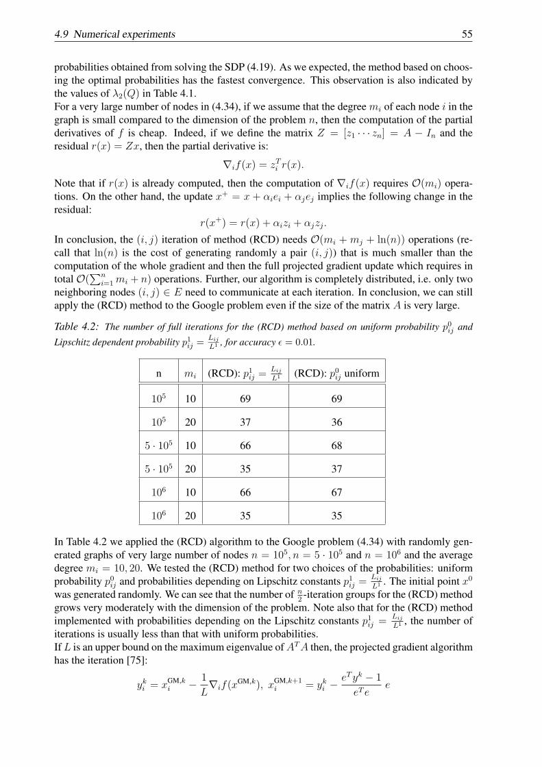
4.9 Numerical experiments 55
probabilities obtained from solving the SDP (4.19). As we expected, the method based on choos-ing the optimal probabilities has the fastest convergence. This observation is also indicated bythe values of λ2(Q) in Table 4.1.For a very large number of nodes in (4.34), if we assume that the degree mi of each node i in thegraph is small compared to the dimension of the problem n, then the computation of the partialderivatives of f is cheap. Indeed, if we define the matrix Z = [z1 · · · zn] = A − In and theresidual r(x) = Zx, then the partial derivative is:
∇if(x) = zTi r(x).
Note that if r(x) is already computed, then the computation of ∇if(x) requires O(mi) opera-tions. On the other hand, the update x+ = x + αiei + αjej implies the following change in theresidual:
r(x+) = r(x) + αizi + αjzj.
In conclusion, the (i, j) iteration of method (RCD) needs O(mi + mj + ln(n)) operations (re-call that ln(n) is the cost of generating randomly a pair (i, j)) that is much smaller than thecomputation of the whole gradient and then the full projected gradient update which requires intotal O(
∑ni=1mi + n) operations. Further, our algorithm is completely distributed, i.e. only two
neighboring nodes (i, j) ∈ E need to communicate at each iteration. In conclusion, we can stillapply the (RCD) method to the Google problem even if the size of the matrix A is very large.
Table 4.2: The number of full iterations for the (RCD) method based on uniform probability p0ij and
Lipschitz dependent probability p1ij =Lij
L1 , for accuracy ϵ = 0.01.
n mi (RCD): p1ij =Lij
L1 (RCD): p0ij uniform
105 10 69 69
105 20 37 36
5 · 105 10 66 68
5 · 105 20 35 37
106 10 66 67
106 20 35 35
In Table 4.2 we applied the (RCD) algorithm to the Google problem (4.34) with randomly gen-erated graphs of very large number of nodes n = 105, n = 5 · 105 and n = 106 and the averagedegree mi = 10, 20. We tested the (RCD) method for two choices of the probabilities: uniformprobability p0ij and probabilities depending on Lipschitz constants p1ij =
Lij
L1 . The initial point x0
was generated randomly. We can see that the number of n2-iteration groups for the (RCD) method
grows very moderately with the dimension of the problem. Note also that for the (RCD) methodimplemented with probabilities depending on the Lipschitz constants p1ij =
Lij
L1 , the number ofiterations is usually less than that with uniform probabilities.IfL is an upper bound on the maximum eigenvalue ofATA then, the projected gradient algorithmhas the iteration [75]:
yki = xGM,ki − 1
L∇if(x
GM,k), xGM,k+1i = yki −
eTyk − 1
eT ee

4.9 Numerical experiments 56
Figure 4.2: Evolution of ∥Axk−xk∥∥xk∥ along full iterations k for the methods: projected gradient,
center-free [23] with Metropolis weights and (RCD) with uniform and Lipschitz dependent prob-abilities (n = 5000 and mi = 10).
0 100 200 300 400 500 600 700 80010
−2
100
k (number of full iterations)
||A*x
k −xk ||/
||xk ||
Gradient method[23] Metropolis
RCD pij=Lij/L1
RCD pij uniform
for all i = 1, · · · , n, so that in order to update the iteration we need to compute the scalarproducts zTi r(x) for all i = 1, · · · , n and update each component of r(x) ∈ Rn, which require intotalO(
∑ni=1mi + n) operations. Furthermore, the computations of the local Lipschitz constant
Li required by algorithm (RCD) can be done locally and very efficiently Li = ∥zi∥2, whilecomputing the global Lipschitz constant L for projected gradient method on problems of verylarge dimension is extremely difficult.From Table 4.2 (for accuracy ϵ = 0.01) we see that for the same number of full iterations theusual projected gradient method would give worse accuracy, e.g. ∥AxGM,35−xGM,35∥
∥xGM,35∥ = 0.463 for
n = 105 and mi = 20. In Fig. 4.2 we plot the evolution of ∥Axk−xk∥∥xk∥ along full iterations k
for the following methods: the distributed algorithm from [121] with the Metropolis weights, thefull projected gradient algorithm and the (RCD) algorithm with uniform and Lipschitz dependentprobabilities for a random generated graph with n = 5000 nodes and the average degree mi =10. We clearly see that the best accuracy is achieved by the (RCD) algorithm with Lipschitzdependent probabilities.
Chapter 5
Random coordinate descent method forlinearly constrained compositeoptimization
In this chapter we propose a variant of the random coordinate descent method for solving linearlyconstrained convex optimization problems with composite objective functions. If the smoothpart of the objective function has Lipschitz continuous gradient, then we prove that our methodobtains an ϵ-optimal solution in O(n2/ϵ) iterations, where n is the number of blocks. For theclass of problems with cheap coordinate derivatives we show that the new method is faster thanmethods based on full-gradient information. Analysis for the rate of convergence in probability isalso provided. For strongly convex functions our method converges linearly. Extensive numericaltests confirm that on very large problems, our method is much more numerically efficient thanmethods based on full gradient information. This chapter is based on paper [70].
5.1 IntroductionLinearly constrained optimization problems with composite objective function arise in manyapplications such as compressive sensing [14], image processing [19], truss topology design [80],distributed control [65], support vector machines [109], traffic equilibrium and network flowproblems [9] and many other areas.In this chapter we present a random coordinate descent method suited for large scale problemswith composite objective function. Moreover, we focus on linearly coupled constrained opti-mization problems (i.e., the constraint set is coupled through linear equalities). Note that themodel considered in this chapter is more general than the one from Chapters 3 and 4, since weallow composite objective functions. We prove for our method an expected convergence rateof order O(n2
k), where n is number of blocks and k is the iteration counter. We show that for
functions with cheap coordinate derivatives the new method is much faster, either in worst casecomplexity analysis, or numerical implementation, than schemes based on full gradient infor-mation (e.g., coordinate gradient descent method developed in [107, 108]). But our method alsooffers other important advantages, e.g., due to the randomization, our algorithm is easier to an-alyze and implement, it leads to more robust output and is adequate for modern computationalarchitectures (e.g, parallel or distributed architectures). Analysis for rate of convergence in prob-ability is also provided. For strongly convex functions we prove that the new method convergeslinearly. We also provide extensive numerical simulations and compare our algorithm against
57

5.2 Problem formulation 58
state-of-the-art methods from the literature on three large-scale applications: support vector ma-chine, the Chebyshev center of a set of points and random generated optimization problems withan ℓ1-regularization term.The chapter is organized as follows. In order to present our main results, we introduce somenotations and assumptions for our optimization model in Section 5.2. In Section 5.4 we presentthe new random coordinate descent (RCD) algorithm. The main results of the chapter can befound in Sections 5.5–5.7, where we derive the rate of convergence in expectation, probabilityand for the strongly convex case. In Section 5.8 we generalize the algorithm and extend theprevious results to a more general model. We also analyze its complexity and compare it withother methods from the literature, in particular the coordinate descent method of Tseng [107,108] in Section 5.9. Finally, we test the practical efficiency of our algorithm through extensivenumerical experiments in Section 5.10.
5.2 Problem formulationWe work in the space RN composed of column vectors. For x, y ∈ RN we denote:
⟨x, y⟩ =n∑
i=1
x(i)y(i).
We use the same notation ⟨·, ·⟩ for spaces of different dimensions. If we fix a norm ∥·∥ in RN ,then its dual norm is defined by:
∥y∥∗ = max∥x∥=1
⟨y, x⟩.
We assume that the entire space dimension is decomposable into n blocks:
N =n∑
i=1
ni.
We denote by Ui the blocks of the identity matrix:
IN = [U1 . . . Un] ,
where Ui ∈ RN×ni . For some vector x ∈ RN , we use the notation x(i) ∈ Rni for the ith blockof the vector x, i.e. x(i) = UT
i x, and xi ∈ R for the ith coordinate of vector x. Moreover, weintroduce a two-blocks nonzero vector xij ∈ RN associated to x, defined as: xij = Uix(i) +Ujx(j). We also define ∇if(x) = UT
i ∇f(x) as the ith block in the gradient of the function f atx. Similarly,∇ijf(x) = Ui∇if(x)+Uj∇jf(x) ∈ RN . We denote by supp(x) the set of indexescorresponding to nonzero coordinates in x. Given a matrix A ∈ Rm×n, we denote its nullspaceby Null(A). In the rest of the chapter we consider local Euclidean norms in all spaces Rni , i.e.,∥∥x(i)∥∥ =
√(x(i))Tx(i) for all x(i) ∈ Rni and i = 1, . . . , n.
The basic problem of interest in this chapter is the following convex minimization problem withcomposite objective function:
minx∈RN
F (x) (:= f(x) + h(x))
s.t.: aTx = 0,(5.1)
where f : RN → R is a smooth convex function defined by a black-box oracle, h : RN →R is a general closed convex function and a ∈ RN . Further, we assume that function h is
5.2 Problem formulation 59
coordinatewise separable and simple (by simple we mean that we can find a closed-form solutionfor the minimization of h with some simple auxiliary function). Special cases of this modelinclude linearly constrained smooth optimization (where h ≡ 0) which was analyzed in [59,68, 121], support vector machines (where h is the indicator function of some box constraintset) [35, 50] and composite optimization (where a = 0) [52, 77, 93, 106–109].For model (6.1) we make the following assumptions:
Assumption 5.2.1 The smooth and nonsmooth parts of the objective function in optimizationmodel (6.1) satisfy the following properties:
(i) Function f is convex and has block-coordinate Lipschitz continuous gradient:∥∥∇if(x+ Uis(i))−∇if(x)∥∥∗ ≤ Li
∥∥s(i)∥∥ ∀x ∈ RN , s(i) ∈ Rni , i = 1, . . . , n.
(ii) The nonsmooth function h is convex and coordinatewise separable, i.e. h(x) =N∑i=1
hi(xi),
where hi : R → R for all i = 1, . . . , N .
Assumption 5.2.1 (i) is typical for composite optimization, see e.g., [59,76,78,108]. Assumption5.2.1 (ii) covers many applications as we further exemplify. A special case of coordinatewiseseparable function that has attracted a lot of attention in the area of signal processing and datamining is the ℓ1-regularization [14]:
h(x) = λ ∥x∥1 , (5.2)
where λ > 0. Often, a large λ factor induces sparsity in the solution of optimization problem(6.1). Note that the function h in (5.2) belongs to the general class of coordinatewise separablepiecewise linear/quadratic functions with O(1) pieces. Another special case is the box indicatorfunction, i.e.:
h(x) = 1[l,u] =
0, l ≤ x ≤ u
∞, otherwise.(5.3)
Adding box constraints to a quadratic objective function f in (6.1) leads e.g., to support vectormachine (SVM) problems [16,109]. The reader can easily find many other examples of functionh satisfying Assumption 5.2.1 (ii).Based on Assumption 1 (i), the following inequality can be derived [75]:
f(x+ Uis(i)) ≤ f(x) + ⟨∇if(x), s(i)⟩+Li
2
∥∥s(i)∥∥2 ∀x ∈ RN , s(i) ∈ Rni . (5.4)
In the sequel, we use the notation:L = max
1≤i≤nLi.
For α ∈ [0, 1] we introduce the following extended norm on RN :
∥x∥α =
(n∑
i=1
Lαi
∥∥x(i)∥∥2)12
and its dual norm
∥y∥∗α =
(n∑
i=1
1
Lαi
(∥∥y(i)∥∥∗)2)12
.
5.2 Problem formulation 60
Note that these norms satisfy the Cauchy-Schwartz inequality:
∥x∥α ∥y∥∗α ≥ ⟨x, y⟩ ∀x, y ∈ RN .
Recall that for a vector x ∈ RN such that x =∑n
i=1 Uix(i), we define an extended two-blocksnonzero vector on the components (i, j) as follows: xij = Uix(i)+Ujx(j). Based on Assumption5.2.1 (ii) we can derive from (5.4) the following result:
Lemma 5.2.2 Let the function f be convex and satisfy Assumption 5.2.1. Then, f has compo-nentwise Lipschitz continuous gradient w.r.t. every pair (i, j) with i = j, i.e.:
∥∇ijf(x+ sij)−∇ijf(x)∥∗α ≤ Lαij ∥sij∥α ∀x ∈ RN , s(i) ∈ Rni , s(j) ∈ Rnj ,
where we define Lαij = L1−α
i + L1−αj > 0 and sij = Uis(i) + Ujs(j) ∈ RN .
Proof : Let f ∗ = minx∈RN
f(x). Based on (5.4) we have for any pair (i, j):
f(x)− f ∗ ≥ maxl∈1,...N
1
2Ll
(∥∇lf(x)∥∗)2 ≥ maxl∈i,j
1
2Ll
(∥∇lf(x)∥∗)2
≥ 1
2(L1−αi + L1−α
j
) ( 1
Lαi
(∥∇if(x)∥∗)2 +1
Lαj
(∥∇jf(x)∥∗)2)
=1
2Lαij
(∥∇ijf(x)∥∗α
)2,
where in the third inequality we used that αa + (1 − α)b ≤ maxa, b for all α ∈ [0, 1]. Now,note that for any vector with two nonzero blocks of the form yij = Uiy(i) + Ujy(j), the functiong1(yij) = f(x+ yij − xij)− f(x)− ⟨∇f(x), yij − xij⟩ satisfies the Assumption 5.2.1 (i). If weapply the above inequality to g1(yij) we get the following relation:
f(x+ yij − xij) ≥ f(x) + ⟨∇f(x), yij − xij⟩+1
2Lαij
(∥∇ijf(x+ yij − xij)−∇ijf(x)∥∗α
)2.
On the other hand, applying the same inequality to g2(xij) = f(x)− f(x+ yij−xij)+ ⟨∇f(x+yij − xij), yij − xij⟩, which also satisfies Assumption 5.2.1 (i), we have:
f(x) ≥ f(x+ yij − xij) + ⟨∇f(x+yij − xij), yij − xij⟩+1
2Lαij
(∥∇ijf(x+ yij − xij)−∇ijf(x)∥∗α
)2.
Further, denoting sij = yij − xij ∈ RN , with only two nonzero blocks s(i) ∈ Rni and s(j) ∈ Rnj ,and adding up the resulting inequalities we get:
1
Lαij
(∥∇ijf(x+ sij)−∇ijf(x)∥∗α
)2 ≤ ⟨∇f(x+ sij)−∇f(x), sij⟩
= ⟨
[∇if(x+ sij)−∇if(x)
∇jf(x+ sij)−∇if(x)
],
[s(i)
s(j)
]⟩
≤ ∥∇ijf(x+ sij)−∇ijf(x)∥∗α ∥sij∥α ,
for all x ∈ RN . This relation proves the statement of this lemma. 2
5.3 Previous work 61
It is straightforward to see that we can obtain from Lemma 5.2.2 the following inequality [75]:
f(x+ sij) ≤ f(x) + ⟨∇ijf(x), sij⟩+Lα
ij
2∥sij∥2α , (5.5)
for all α ∈ [0, 1], x ∈ RN , sij ∈ RN , where only blocks s(i) ∈ Rni , s(j) ∈ Rnj of the vector sijare nonzeros, i.e. sij = Uis(i) + Ujs(j).
5.3 Previous workWe briefly review some well-known methods from the literature for solving the optimizationmodel (6.1). In [53, 108, 109] Tseng studied optimization problems in the form (6.1) and devel-oped a (block) coordinate gradient descent(CGD) method based on the Gauss-Southwell choicerule. The main requirement for the (CGD) iteration is the solution of the following problem:given a feasible x and a working set of indexes J , the update direction is defined by
dH(x;J ) = arg mins∈RN
f(x) + ⟨∇f(x), s⟩+ 1
2⟨Hs, s⟩+ h(x+ s)
s.t.: aT s = 0, s(j) = 0 ∀j /∈ J ,(5.6)
where H ∈ RN×N is a symmetric matrix chosen at the initial step of the algorithm.
Algorithm (CGD):1. Choose a nonempty set of indices J k ⊂ 1, . . . , n with respect to the
Gauss-Southwell rule
2. Solve (5.6) with x = xk, J = J k, H = Hk to obtain dk = dHk(xk;J k)
3. Choose stepsize αk > 0 and set xk+1 = xk + αkdk.
In [108], the authors proved for the particular case when function h is piece-wise linear/quadraticwith O(1) pieces that an ϵ-optimal solution is attained in O(NLR2
0
ϵ) iterations, where R0 denotes
the Euclidean distance from the initial point to some optimal solution. Also, in [108] the authorsderive estimates of orderO(N) on the computational complexity of each iteration for this choiceof h.Furthermore, for a quadratic function f and a box indicator function h (e.g., support vectormachine (SVM) applications) one of the first decomposition approaches developed similar to(RCD) is Sequential Minimal Optimization (SMO) [86]. SMO consists of choosing at eachiteration two scalar coordinates with respect to some heuristic rule based on KKT conditions andsolving the small QP subproblem obtained through the decomposition process. However, the rateof convergence is not provided for the SMO algorithm. But the numerical experiments show thatthe method is very efficient in practice due to the closed form solution of the QP subproblem. Listand Simon [50] proposed a variant of block coordinate descent method for which an arithmeticcomplexity of order O(N
2LR20
ϵ) is proved on a quadratic model with a box indicator function and
generalized linear constraints. Later, Hush et al. [35] presented a more practical decompositionmethod which attains the same complexity as the previous methods.A random coordinate descent algorithm for model (6.1) with a = 0 and h being the indicatorfunction for a Cartesian product of sets was analyzed by Nesterov in [76]. The generalization ofthis algorithm to more general composite objective functions has been studied in [93]. However,
5.4 Random coordinate descent algorithm 62
none of these papers studied the application of coordinate descent algorithms to linearly coupledconstrained optimization models. Similar random coordinate descent algorithms as the (RCD)method described in the present chapter, for optimization problems with smooth objective andlinearly coupled constraints, has been developed and analyzed in Chapters 3 and 4. We furtherextend these results to linearly constrained composite objective function optimization and pro-vide in the sequel the convergence rate analysis for the previously presented variant of the (RCD)method (see Algorithm 1 (RCD) below).
5.4 Random coordinate descent algorithmIn this section we introduce a variant of Random Coordinate Descent (RCD) method for solvingproblem (6.1) that performs a minimization step with respect to two block variables at eachiteration. The coupling constraint (that is, the weighted sum constraint aTx = 0) prevents thedevelopment of an algorithm that performs a minimization with respect to only one variable ateach iteration. We will therefore be interested in the restriction of the objective function f onfeasible directions consisting of at least two nonzero (block) components.Let (i, j) be a two dimensional random variable, where i, j ∈ 1, . . . , n with i = j and pikjk =Pr((i, j) = (ik, jk)) be its probability distribution. We denote with I the set of all such possiblepairs, i.e. I = (i, j) : i, j = 1, . . . , n, i = j. Given a feasible x, two blocks are chosenrandomly with respect to a given probability distribution pij and a quadratic model derived fromthe composite objective function is minimized with respect to these coordinates. Our method hasthe following iteration: given a feasible initial point x0, that is aTx0 = 0, then for all k ≥ 0
Algorithm 1 (RCD)1. Choose randomly two coordinates (ik, jk) ∈ I with probability pikjk2. Set xk+1 = xk + Uikd(ik) + Ujkd(jk),
where the directions d(ik) and d(jk) are chosen as follows: if we use for simplicity the notation(i, j) instead of (ik, jk), the direction dij = Uid(i) + Ujd(j) is given by
dij = arg minsij=Uis(i)+Ujs(j)
f(xk) + ⟨∇ijf(xk), sij⟩+
Lαij
2∥sij∥2α + h(xk + sij)
s.t.: aT(i)s(i) + aT(j)s(j) = 0,
(5.7)
where a(i) ∈ Rni and a(j) ∈ Rnj are the ith and jth blocks of vector a, respectively. Clearly, inour algorithm we maintain feasibility at each iteration, i.e. aTxk = 0 for all k ≥ 0.
Remark 5.4.1
(i) Note that for the scalar case (i.e., N = n) and h given by (5.2) or (5.3), the directiondij in (6.4) can be computed in closed form. For the block case (i.e., ni > 1 for alli) and if h is a coordinatewise separable, strictly convex and piece-wise linear/quadraticfunction with O(1) pieces (e.g., h given by (5.2)), there are algorithms for solving theabove subproblem in linear-time (i.e., O(ni + nj) operations) [108]. Also for h given by(5.3), there exist in the literature algorithms for solving the subproblem (6.4) with overallcomplexity O(ni + nj) [7, 40].
5.5 Convergence rate in expectation 63
(ii) In algorithm (RCD) we consider (i, j) = (j, i) and i = j. Moreover, we know that thecomplexity of choosing randomly a pair (i, j) with a uniform probability distribution re-quires O(1) operations. 2
We assume that random variables (ik, jk)k≥0 are i.i.d. In the sequel, we use notation ηk for theentire history of random pair choices and ϕk for the expected value of the objective function w.r.t.ηk, i.e.:
ηk = (i0, j0), . . . , (ik−1, jk−1) and ϕk = E[F (xk)
].
In the following sections we derive the convergence rate of Algorithm 1 (RCD) for compositeoptimization model (6.1) in expectation, probability and for strongly convex functions.
5.5 Convergence rate in expectationIn this section we study the rate of convergence in expectation of algorithm (RCD). We consideruniform probability distribution, i.e., the event of choosing a pair (i, j) can occur with probabil-ity:
pij =2
n(n− 1),
since we assume that (i, j) = (j, i) and i = j ∈ 1, . . . , n (see Remark 5.4.1 (ii)). In order toprovide the convergence rate of our algorithm, first we have to define the conformal realizationof a vector introduced in [98].
Definition 5.5.1 Let d, d′ ∈ RN , then the vector d′ is conformal to d if:
supp(d′) ⊆ supp(d) and d′jdj ≥ 0 ∀j = 1, . . . , N.
For a given matrix A ∈ Rm×N , with m ≤ N , we introduce the notion of elementary vectorsdefined as:
Definition 5.5.2 An elementary vector of Null(A) is a vector d ∈ Null(A) for which there isno nonzero vector d′ ∈ Null(A) conformal to d and supp(d′) = supp(d).
Based on Exercise 10.6 in [98] we state the following lemma:
Lemma 5.5.3 [98] Given d ∈ Null(A), if d is an elementary vector, then |supp(d)| ≤rank(A) + 1 ≤ m+ 1. Otherwise, d has a conformal realization:
d = d1 + · · ·+ dq,
where q ≥ 1 and dt ∈ Null(A) are elementary vectors conformal to d for all t = 1, . . . , q.
For the scalar case, i.e., N = n and m = 1, the method provided in [108] finds a conformal real-ization with dimension q ≤ |supp(d)| − 1 within O(N) operations. We observe that elementaryvectors dt in Lemma 5.5.3 for the case m = 1 (i.e., A = aT ) have at most 2 nonzero components.Our convergence analysis is based on the following lemma, whose proof can be found in [108,Lemma 6.1]:
5.5 Convergence rate in expectation 64
Lemma 5.5.4 Let h be coordinatewise separable and convex. For any y, y + d ∈ dom h, let dbe expressed as d = d1 + · · ·+ dq for some q ≥ 1 and some nonzero dt ∈ RN conformal to d fort = 1, . . . , q. Then, we have:
h(y + d)− h(y) ≥q∑
t=1
(h(y + dt)− h(y)
).
For the simplicity of the analysis we introduce the following linear subspaces:
Sij =d ∈ RN : d = Uid(i) + Ujd(j), a
Tijd = 0
and S =
d ∈ RN : aTd = 0
.
We denote by F ∗ and X∗ the optimal value and the optimal solution set for problem (6.1),respectively. We also introduce the maximal residual defined in terms of the norm ∥ · ∥α:
Rα = maxx
maxx∗∈X∗
∥x− x∗∥α : F (x) ≤ F (x0)
,
which measures the size of the level set of F given by x0. We assume that this distance is finitefor the initial iterate x0.Now, we prove the main result of this section:
Theorem 5.5.5 Let F satisfy Assumption 5.2.1. Then, the random coordinate descent algorithm(RCD) based on the uniform distribution generates a sequence xk satisfying the following con-vergence rate for the expected values of the objective function:
ϕk − F ∗ ≤ n2L1−αR2α
k + n2L1−αR2α
F (x0)−F ∗
,
where we recall that ϕk = E[F (xk)
].
Proof : For simplicity of the exposition we use the following notation: given the current iteratex, denote x+ = x+Uid(i)+Ujd(j) the next iterate, where directions (d(i), d(j)) are given by (6.4)for some random chosen pair (i, j) w.r.t. uniform distribution. For brevity, we also adapt thenotation of expectation upon the entire history, i.e. (ϕ, ϕ+, η) instead of (ϕk, ϕk+1, ηk). Based on(5.5) we derive:
F (x+) ≤ f(x) + ⟨∇ijf(x), dij⟩+Lαij
2∥dij∥2α + h(x+ dij)
(6.4)= min
sij∈Sij
f(x) + ⟨∇ijf(x), sij⟩+Lαij
2∥sij∥2α + h(x+ sij).
We now take expectation in both sides conditioned on η and note that (i, j) is independent on thepast η, while x is fully determined by η, according to our convention. Recalling that pij = 2
n(n−1),
we get:
E[F (x+)
∣∣η] ≤ E
[min
sij∈Sij
f(x) +⟨∇ijf(x), sij⟩+Lαij
2∥sij∥2α + h(x+ sij)
∣∣∣η]≤ E
[f(x) + ⟨∇ijf(x), sij⟩+
Lαij
2∥sij∥2α + h(x+ sij)
∣∣∣η]=
2
N(N−1)∑
(i,j)∈I
(f(x)+⟨∇ijf(x), sij⟩+
Lαij
2∥sij∥2α+h(x+ sij)
)
=f(x)+2
N(N−1)
⟨∇f(x), ∑(i,j)∈I
sij⟩+∑
(i,j)∈I
Lαij
2∥sij∥2α+
∑(i,j)∈I
h(x+sij)
,(5.8)

5.5 Convergence rate in expectation 65
for all possible sij ∈ Sij , with (i, j) ∈ I.Based on Lemma 5.5.3 for m = 1, it follows that any d ∈ S has a conformal realization defined
by d =q∑
t=1
dt, where the vectors dt ∈ S are conformal to d and have only two nonzero com-
ponents. Thus, for any t = 1, . . . , q there is a pair (i, j) such that dt ∈ Sij . Therefore, for anyd ∈ S we can choose an appropriate set of pairs (i, j) and vectors sdij ∈ Sij conformal to d suchthat d =
∑(i,j)∈I
sdij . As we have seen, the above chain of relations in (5.8) holds for all the pairs
(i, j) ∈ I and vectors sij ∈ Sij . Therefore, it also holds for the set of pairs (i, j) and vectors sdijsuch that d =
∑(i,j)∈I
sdij . In conclusion, we have from (5.8) that:
E[F (x+)
∣∣η]≤f(x) + 2
n(n− 1)
⟨∇f(x),∑(i,j)∈I
sdij⟩+∑
(i,j)∈I
Lαij
2
∥∥sdij∥∥2α +∑
(i,j)∈I
h(x+ sdij)
,for all d ∈ S, where we set sdij = 0 for those pair components (i, j) ∈ I that are not in theconformal realization of the vector d. Moreover, observing that Lα
ij ≤ 2L1−α and applyingLemma ?? in the previous inequality for coordinatewise separable functions ∥·∥2α, with y = 0,and for h(·), with y = x respectively, we obtain:
E[F (x+)
∣∣η]≤f(x)+ 2
n(n− 1)
(⟨∇f(x),
∑(i,j)∈I
sdij⟩+∑
(i,j)∈I
Lαij
2
∥∥sdij∥∥2α +∑
(i.j)∈I
h(x+ sdij)),
Lemma 3
≤ f(x) +2
n(n− 1)
(⟨∇f(x),
∑(i,j)∈I
sdij⟩+ L1−α∥∑
(i,j)∈I
sdij∥2α+
h(x+∑
(i,j)∈I
sdij)+(n(n− 1)
2− 1)h(x)
)d=
∑(i,j)∈I
sdij
=(1− 2
n(n− 1)
)F (x) +
2
n(n− 1)
(f(x) + ⟨∇f(x), d⟩+
L1−α ∥d∥2α+h(x+ d)),
(5.9)
for any d ∈ S. Note that (5.9) holds for every d ∈ S since (5.8) holds for any sij ∈ Sij .Therefore, as (5.9) holds for every vector from the subspace S, it also holds for the followingparticular vector d ∈ S defined as:
d = argmins∈S
f(x) + ⟨∇f(x), s⟩+ L1−α ∥s∥2α + h(x+ s).
Based on this choice and using a similar reasoning as in [78] for proving the convergence rate of
5.5 Convergence rate in expectation 66
gradient type methods for composite objective functions, we derive the following:
f(x) + ⟨∇f(x), d⟩+ L1−α∥∥∥d∥∥∥2
α+ h(x+ d)
= miny∈S
f(x) + ⟨∇f(x), y − x⟩+ L1−α ∥y − x∥2α + h(y)
≤ miny∈S
F (y) + L1−α ∥y − x∥2α
≤ minβ∈[0,1]
F (βx∗ + (1− β)x) + β2L1−α ∥x− x∗∥2α
≤ minβ∈[0,1]
F (x)− β(F (x)− F ∗) + β2L1−αR2α
= F (x)− (F (x)− F ∗)2
L1−αR2α
,
where in the first inequality we used the convexity of f while in the second and third inequalitieswe used basic optimization arguments. Therefore, at each iteration k the following inequalityholds:
E[F (xk+1)
∣∣ηk] ≤(1− 2
n(n− 1))F (xk)+
2
n(n− 1)
[F (xk)− (F (xk)− F ∗)2
L1−αR2α
].
Taking expectation with respect to ηk and using convexity properties we get:
ϕk+1 − F ∗ ≤(1− 2
n(n− 1))(ϕk − F ∗)+
2
n(n− 1)
[(ϕk − F ∗)− (ϕk − F ∗)2
L1−αR2α
]≤(ϕk − F ∗)− 2
n(n− 1)
[(ϕk − F ∗)2
L1−αR2α
].
(5.10)
Further, if we denote ∆k = ϕk − F ∗ and γ = n(n− 1)L1−αR2α we get:
∆k+1 ≤ ∆k − (∆k)2
γ.
Dividing both sides with ∆k∆k+1 > 0 and using the fact that ∆k+1 ≤ ∆k we get:
1
∆k+1≥ 1
∆k+
1
γ∀k ≥ 0.
Finally, summing up from 0, . . . , k we easily get the above convergence rate. 2
Let us analyze the convergence rate of our method for the two most common cases of the ex-tended norm on RN introduced in this section: w.r.t. extended Euclidean norm ∥·∥0 = ∥·∥ (i.e.,α = 0) and norm ∥·∥1 (i.e., α = 1). Recall that the norm ∥·∥1 is defined by:
∥x∥21 =n∑
i=1
Li
∥∥x(i)∥∥2 .

5.6 Convergence rate for strongly convex functions 67
Lemma 5.5.6 Under the same assumptions of Theorem 5.5.5, the algorithm (RCD) generates asequence xk such that the expected values of the objective function satisfy the following conver-gence rates for α = 0 and α = 1:
α = 0 : ϕk − F ∗ ≤ n2LR20
k +n2LR2
0
F (x0)−F ∗
,
α = 1 : ϕk − F ∗ ≤ n2R21
k +n2R2
1
F (x0)−F ∗
.
Remark 5.5.7 We usually have R21 ≤ LR2
0 and this shows the advantages that the general norm
∥·∥α has over the Euclidean norm. Indeed, if we denote by r2i = maxx
maxx∗∈X∗
∥∥∥x(i) − x∗(i)∥∥∥2 :
F (x) ≤ F (x0)
, then we can provide upper bounds on R21 ≤
∑ni=1 Lir
2i and R2
0 ≤∑n
i=1 r2i .
Clearly, the following inequality is valid:
n∑i=1
Lir2i ≤
n∑i=1
Lr2i ,
and the inequality holds with equality only for Li = L for all i = 1, . . . , n. We recall thatL = maxi Li. Therefore, in the majority of cases the estimate for the rate of convergence basedon norm ∥·∥1 is much better than that based on the Euclidean norm ∥·∥0. 2
5.6 Convergence rate for strongly convex functionsNow, we assume that the objective function in (6.1) is σα-strongly convex with respect to norm∥·∥α, i.e.:
F (x) ≥ F (y) + ⟨F ′(y), x− y⟩+ σα2∥x− y∥2α ∀x, y ∈ RN , (5.11)
where F ′(y) denotes some subgradient of F at y. Note that if the function f is σ-strongly convexw.r.t. extended Euclidean norm, then we can remark that it is also σα-strongly convex functionw.r.t. norm ∥·∥α and the following relation between the strong convexity constants holds:
σ
Lα
n∑i=1
Lα∥∥x(i) − y(i)∥∥2 ≥ σ
Lα
n∑i=1
Lαi
∥∥x(i) − y(i)∥∥2≥ σα ∥x− y∥2α ,
which leads toσα ≤
σ
Lα.
Taking y = x∗ in (5.11) and from optimality conditions ⟨F ′(x∗), x − x∗⟩ ≥ 0 for all x ∈ S weobtain:
F (x)− F ∗ ≥ σα2∥x− x∗∥2α . (5.12)
Next, we state the convergence result of our algorithm (RCD) for solving the problem (6.1) withσα-strongly convex objective w.r.t. norm ∥·∥α.
5.6 Convergence rate for strongly convex functions 68
Theorem 5.6.1 Under the assumptions of Theorem 5.5.5, let F be also σα-strongly convex w.r.t.∥·∥α. For the sequence xk generated by algorithm (RCD) we have the following rate of conver-gence of the expected values of the objective function:
ϕk − F ∗ ≤(1− 2(1− γ)
n2
)k
(F (x0)− F ∗),
where γ is defined by:
γ =
1− σα
8L1−α , if σα ≤ 4L1−α
2L1−α
σα, otherwise.
Proof : Based on relation (5.9) it follows that:
E[F (xk+1)∣∣ηk] ≤(1− 2
n(n− 1))F (xk)+
2
n(n− 1)mind∈S
(f(xk)+⟨∇f(xk), d⟩+ L1−α ∥d∥2α+h(x
k + d)).
Then, using similar derivation as in Theorem 1 we have:
mind∈S
f(xk) + ⟨∇f(xk), d⟩+ L1−α ∥d∥2α + h(xk + d)
≤ miny∈S
F (y) + L1−α∥∥y − xk∥∥2
α
≤ minβ∈[0,1]
F (βx∗ + (1− β)xk) + β2L1−α∥∥xk − x∗∥∥2
α
≤ minβ∈[0,1]
F (xk)− β(F (xk)− F ∗) + β2L1−α∥∥xk − x∗∥∥2
α
≤ minβ∈[0,1]
F (xk) + β
(2βL1−α
σα− 1
)(F (xk)− F ∗) ,
where the last inequality results from (5.12). The statement of the theorem is obtained by notingthat β∗ = min1, σα
4L1−α and the following subcases:
1. If β∗ = σα
4L1−α and we take the expectation w.r.t. ηk we get:
ϕk+1 − F ∗ ≤(1− σα
4L1−αn2
)(ϕk − F ∗), (5.13)
2. if β∗ = 1 and we take the expectation w.r.t. ηk we get:
ϕk+1 − F ∗ ≤
[1−
2(1− 2L1−α
σα)
n2
](ϕk − F ∗). (5.14)
2

5.7 Convergence rate in probability 69
5.7 Convergence rate in probabilityFurther, we establish some bounds on the required number of iterations for which the generatedsequence xk attains ϵ-accuracy with prespecified probability. In order to prove this result weuse Lemma 3.8.1 from Chapter 3. Based on this lemma we can state the following rate ofconvergence in probability:
Theorem 5.7.1 Let F be a σα-strongly convex function satisfying Assumption 5.2.1 and ρ > 0be the confidence level. Then, the sequence xk generated by algorithm (RCD) using uniformdistribution satisfies the following rate of convergence in probability of the expected values ofthe objective function:
Pr(ϕK − F ∗ ≤ ϵ) ≥ 1− ρ,with K satisfying
K ≥
2n2L1−αR2
α
ϵ
(1 + log 1
ρ
)+ 2− 2n2L1−αR2
α
F (x0)−F ∗ , σα = 0
n2
2(1−γ)log F (x0)−F ∗
ϵρ, σα > 0,
where γ =
1− σα
8L1−α , if σα ≤ 4L1−α
2L1−α
σα, otherwise.
Proof : Based on relation (5.10), we note that taking ξk as ξk = ϕk − F ∗, the properties ofLemma 3.8.1 holds and thus we get the first part of our result. Relations (5.13) and (5.14) in thestrongly convex case are similar instances of Lemma 3.8.1 from which we get the second part ofthe result. 2
5.8 GeneralizationsIn this section we study the optimization problem (6.1), but with general linearly coupling con-straints:
minx∈RN
F (x) (:= f(x) + h(x))
s.t.: Ax = 0,(5.15)
where the functions f and h satisfy Assumption 5.2.1 and A ∈ Rm×N is a matrix with 1 < m ≤N . There are very few attempts to solve this problem through coordinate descent strategies andup to our knowledge the only complexity result can be found in [108].For the simplicity of the exposition, we work in this section with the standard Euclidean norm,denoted by ∥·∥0, on the extended space RN . We consider the set of all (m+1)-tuples of the formN = (i1, . . . , im+1), where ij ∈ 1, . . . , n for all j = 1, . . . ,m + 1. Also, we define pN asthe probability distribution associated with (m+1)-tuples of the formN . Given this probabilitydistribution pN , for this general optimization problem (5.15) we propose the following randomcoordinate descent algorithm:
Algorithm 2 (RCD)N
1. Choose randomly a set of (m+ 1)-tuple Nk = (i1k, . . . , im+1k )
with probability pNk
2. Set xk+1 = xk + dNk,
5.9 Complexity analysis and comparison with other approaches 70
where the direction dNkis chosen as follows:
dNk= arg min
s∈RNf(xk) + ⟨∇f(xk), s⟩+ LNk
2∥s∥20 + h(xk + s)
s.t.: As = 0, s(i) = 0 ∀i /∈ Nk.
We can easily see that the linearly coupling constraints Ax = 0 prevent the development ofan algorithm that performs at each iteration a minimization with respect to less than m + 1coordinates. Therefore we are interested in the class of iteration updates which restricts theobjective function on feasible directions that consist of at least m+ 1 (block) components.Further, we redefine the subspace S as S = s ∈ RN : As = 0 and additionally we denote thelocal subspace SN = s ∈ RN : As = 0, s(i) = 0 ∀i ∈ N. Note that we still consider anordered (m + 1)-tuple Nk = (i1k, . . . , i
m+1k ) such that ipk = ilk for all p = l. We observe that for
a general matrix A, the previous subproblem does not necessarily have a closed form solution.However, when h is coordinatewise separable, strictly convex and piece-wise linear/quadraticwith O(1) pieces (e.g., h given by (5.2)) there are efficient algorithms for solving the previoussubproblem in linear-time [108]. Moreover, when h is the box indicator function (i.e., h givenby (5.3)) we have the following: in the scalar case (i.e., N = n) the subproblem has a closedform solution; for the block case (i.e., n < N ) there exist linear-time algorithms for solving thesubproblem within O(
∑i∈Nk
ni) operations [7]. Through a similar reasoning as in Lemma 5.2.2we can derive that given a set of indices N = (i1, . . . , iq), with q ≥ 2, the following relationholds:
f(x+ dN ) ≤ f(x) + ⟨∇f(x), dN ⟩+LN
2∥dN∥20 , (5.16)
for all x ∈ RN and dN ∈ RN with nonzero entries only on the blocks i1, . . . , iq. Here, LN =Li1 + · · · + Liq . Moreover, based on Lemma 5.5.3 it follows that any d ∈ S has a conformalrealization defined by d =
∑qt=1 d
t, where the elementary vectors dt ∈ S are conformal to d andhave at most m + 1 nonzeros. Therefore, any vector d ∈ S can be generated by d =
∑N sN ,
where the vectors sN ∈ SN have at most m+ 1 nonzero blocks and are conformal to d. We nowpresent the main convergence result for this method.
Theorem 5.8.1 Let F satisfy Assumption 5.2.1. Then, the random coordinate descent algorithm(RCD)N that chooses uniformly at each iterationm+1 blocks generates a sequence xk satisfyingthe following rate of convergence for the expected values of the objective function:
ϕk − F ∗ ≤ nm+1LR20
k +nm+1LR2
0
F (x0)−F ∗
.
Proof : The proof is similar to that of Theorem 5.5.5 and we omit it here for brevity. 2
5.9 Complexity analysis and comparison with other ap-proaches
In this section we analyze the total complexity (arithmetic complexity [75]) of algorithm (RCD)based on extended Euclidean norm for optimization problem (6.1) and compare it with othercomplexity estimates. Tseng presented in [108] the first complexity bounds for the (CGD)method applied to our optimization problem (6.1). Up to our knowledge there are no othercomplexity results for coordinate descent methods on the general optimization model (6.1).
5.9 Complexity analysis and comparison with other approaches 71
Note that the algorithm (RCD) has an overall complexity w.r.t. extended Euclidean norm givenby:
O(n2LR2
0
ϵ
)O(iRCD),
whereO(iRCD) is the complexity per iteration of algorithm (RCD). On the other hand, algorithm(CGD) has the following complexity estimate:
O(NLR2
0
ϵ
)O(iCGD),
where O(iCGD) is the iteration complexity of algorithm (CGD). Based on the particularities andcomputational effort of each method, we will show in the sequel that for some optimizationmodels arising in real-world applications the arithmetic complexity of (RCD) method is lowerthan that of (CGD) method. For certain instances of problem (6.1) we have that the computa-tion of the coordinate directional derivative of the smooth component of the objective functionis much more simpler than the function evaluation or directional derivative along an arbitrarydirection. Note that the iteration of algorithm (RCD) uses only a small number of coordinatedirectional derivatives of the smooth part of the objective, in contrast with the (CGD) iterationwhich requires the full gradient. Thus, we estimate the arithmetic complexity of these two meth-ods applied to a class of optimization problems containing instances for which the directionalderivative of objective function can be computed cheaply. We recall that the process of choosinga uniformly random pair (i, j) in our method requires O(1) operations.Let us structure a general coordinate descent iteration in two phases:Phase 1: Gather first-order information to form a quadratic approximation of the original opti-mization problem.Phase 2: Solve a quadratic optimization problem using data acquired at Phase 1 and update thecurrent vector.Both algorithms (RCD) and (CGD) share this structure but, as we will see, there is a gap betweencomputational complexities. We analyze the following example:
f(x) =1
2xTZTZx+ qTx, (5.17)
where Z =[z1 . . . zN
]∈ Rm×N has sparse columns, with an average p << N nonzero entries
on each column zi for all i = 1, . . . , N . A particular case of this class of functions is f(x) =12∥Zx− q∥2, which has been considered for numerical experiments in [59,76,93]. The problem
(6.1), with the aforementioned structure (5.17) of the smooth part of the objective function, arisesin many applications: e.g., linear SVM [109], truss topology [80], internet (Google problem)[59, 76], Chebyshev center problems [122], etc. The reader can easily find many other examplesof optimization problems with cheap coordinate directional derivatives.Further, we estimate the iteration complexity of the algorithms (RCD) and (CGD). Given a fea-sible x, from the expression
∇if(x) = ⟨zi, Zx⟩+ qi,
we note that if the residual r(x) = Zx is already known, then the computation of∇if(x) requiresO(p) operations. We consider that the dimension ni of each block is of order O(N
n). Thus,
the (RCD) method updates the current point x on O(Nn) coordinates and summing up with the
computation of the new residual r(x+) = Zx+, which in this case requiresO(pNn) operations, we
conclude that up to this stage, the iteration of (RCD) method has numerical complexity O(pNn).
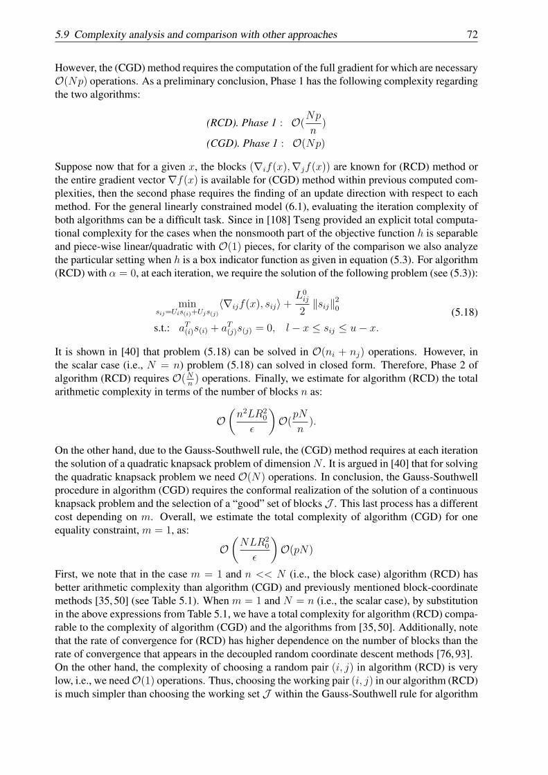
5.9 Complexity analysis and comparison with other approaches 72
However, the (CGD) method requires the computation of the full gradient for which are necessaryO(Np) operations. As a preliminary conclusion, Phase 1 has the following complexity regardingthe two algorithms:
(RCD). Phase 1 : O(Npn
)
(CGD). Phase 1 : O(Np)
Suppose now that for a given x, the blocks (∇if(x),∇jf(x)) are known for (RCD) method orthe entire gradient vector ∇f(x) is available for (CGD) method within previous computed com-plexities, then the second phase requires the finding of an update direction with respect to eachmethod. For the general linearly constrained model (6.1), evaluating the iteration complexity ofboth algorithms can be a difficult task. Since in [108] Tseng provided an explicit total computa-tional complexity for the cases when the nonsmooth part of the objective function h is separableand piece-wise linear/quadratic with O(1) pieces, for clarity of the comparison we also analyzethe particular setting when h is a box indicator function as given in equation (5.3). For algorithm(RCD) with α = 0, at each iteration, we require the solution of the following problem (see (5.3)):
minsij=Uis(i)+Ujs(j)
⟨∇ijf(x), sij⟩+L0
ij
2∥sij∥20
s.t.: aT(i)s(i) + aT(j)s(j) = 0, l − x ≤ sij ≤ u− x.(5.18)
It is shown in [40] that problem (5.18) can be solved in O(ni + nj) operations. However, inthe scalar case (i.e., N = n) problem (5.18) can solved in closed form. Therefore, Phase 2 ofalgorithm (RCD) requires O(N
n) operations. Finally, we estimate for algorithm (RCD) the total
arithmetic complexity in terms of the number of blocks n as:
O(n2LR2
0
ϵ
)O(pN
n).
On the other hand, due to the Gauss-Southwell rule, the (CGD) method requires at each iterationthe solution of a quadratic knapsack problem of dimensionN . It is argued in [40] that for solvingthe quadratic knapsack problem we need O(N) operations. In conclusion, the Gauss-Southwellprocedure in algorithm (CGD) requires the conformal realization of the solution of a continuousknapsack problem and the selection of a “good” set of blocks J . This last process has a differentcost depending on m. Overall, we estimate the total complexity of algorithm (CGD) for oneequality constraint, m = 1, as:
O(NLR2
0
ϵ
)O(pN)
First, we note that in the case m = 1 and n << N (i.e., the block case) algorithm (RCD) hasbetter arithmetic complexity than algorithm (CGD) and previously mentioned block-coordinatemethods [35, 50] (see Table 5.1). When m = 1 and N = n (i.e., the scalar case), by substitutionin the above expressions from Table 5.1, we have a total complexity for algorithm (RCD) compa-rable to the complexity of algorithm (CGD) and the algorithms from [35, 50]. Additionally, notethat the rate of convergence for (RCD) has higher dependence on the number of blocks than therate of convergence that appears in the decoupled random coordinate descent methods [76, 93].On the other hand, the complexity of choosing a random pair (i, j) in algorithm (RCD) is verylow, i.e., we needO(1) operations. Thus, choosing the working pair (i, j) in our algorithm (RCD)is much simpler than choosing the working set J within the Gauss-Southwell rule for algorithm
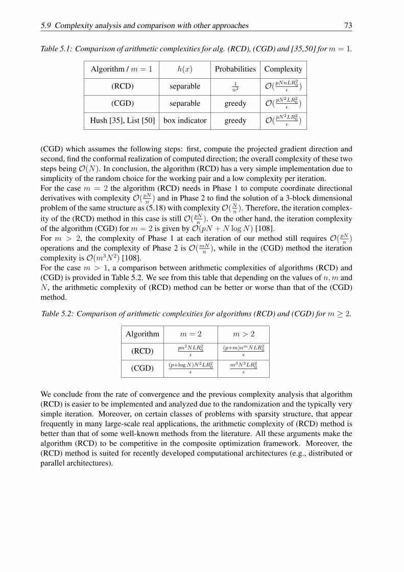
5.9 Complexity analysis and comparison with other approaches 73
Table 5.1: Comparison of arithmetic complexities for alg. (RCD), (CGD) and [35,50] form = 1.
Algorithm / m = 1 h(x) Probabilities Complexity
(RCD) separable 1n2 O(pNnLR2
0
ϵ)
(CGD) separable greedy O(pN2LR2
0
ϵ)
Hush [35], List [50] box indicator greedy O(pN2LR2
0
ϵ)
(CGD) which assumes the following steps: first, compute the projected gradient direction andsecond, find the conformal realization of computed direction; the overall complexity of these twosteps being O(N). In conclusion, the algorithm (RCD) has a very simple implementation due tosimplicity of the random choice for the working pair and a low complexity per iteration.For the case m = 2 the algorithm (RCD) needs in Phase 1 to compute coordinate directionalderivatives with complexity O(pN
n) and in Phase 2 to find the solution of a 3-block dimensional
problem of the same structure as (5.18) with complexityO(Nn). Therefore, the iteration complex-
ity of the (RCD) method in this case is still O(pNn). On the other hand, the iteration complexity
of the algorithm (CGD) for m = 2 is given by O(pN +N logN) [108].For m > 2, the complexity of Phase 1 at each iteration of our method still requires O(pN
n)
operations and the complexity of Phase 2 is O(mNn), while in the (CGD) method the iteration
complexity is O(m3N2) [108].For the case m > 1, a comparison between arithmetic complexities of algorithms (RCD) and(CGD) is provided in Table 5.2. We see from this table that depending on the values of n,m andN , the arithmetic complexity of (RCD) method can be better or worse than that of the (CGD)method.
Table 5.2: Comparison of arithmetic complexities for algorithms (RCD) and (CGD) for m ≥ 2.
Algorithm m = 2 m > 2
(RCD) pn2NLR20
ϵ
(p+m)nmNLR20
ϵ
(CGD) (p+logN)N2LR20
ϵ
m3N3LR20
ϵ
We conclude from the rate of convergence and the previous complexity analysis that algorithm(RCD) is easier to be implemented and analyzed due to the randomization and the typically verysimple iteration. Moreover, on certain classes of problems with sparsity structure, that appearfrequently in many large-scale real applications, the arithmetic complexity of (RCD) method isbetter than that of some well-known methods from the literature. All these arguments make thealgorithm (RCD) to be competitive in the composite optimization framework. Moreover, the(RCD) method is suited for recently developed computational architectures (e.g., distributed orparallel architectures).
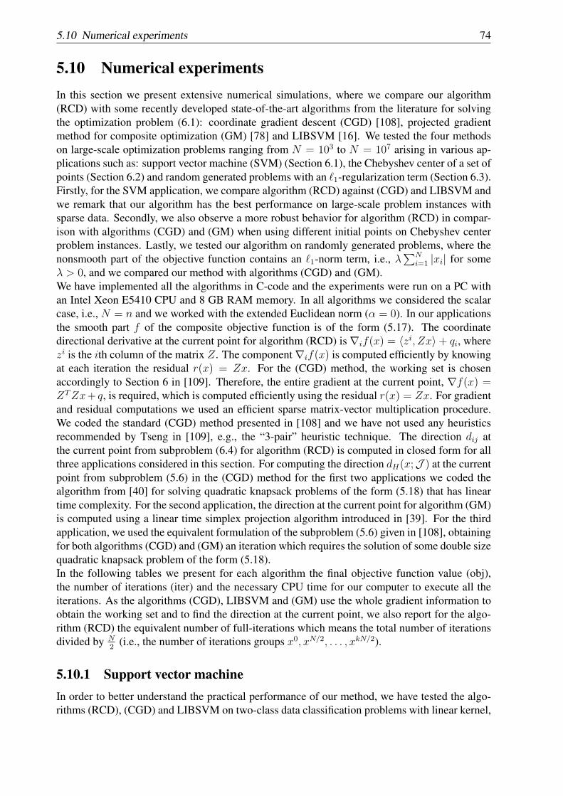
5.10 Numerical experiments 74
5.10 Numerical experimentsIn this section we present extensive numerical simulations, where we compare our algorithm(RCD) with some recently developed state-of-the-art algorithms from the literature for solvingthe optimization problem (6.1): coordinate gradient descent (CGD) [108], projected gradientmethod for composite optimization (GM) [78] and LIBSVM [16]. We tested the four methodson large-scale optimization problems ranging from N = 103 to N = 107 arising in various ap-plications such as: support vector machine (SVM) (Section 6.1), the Chebyshev center of a set ofpoints (Section 6.2) and random generated problems with an ℓ1-regularization term (Section 6.3).Firstly, for the SVM application, we compare algorithm (RCD) against (CGD) and LIBSVM andwe remark that our algorithm has the best performance on large-scale problem instances withsparse data. Secondly, we also observe a more robust behavior for algorithm (RCD) in compar-ison with algorithms (CGD) and (GM) when using different initial points on Chebyshev centerproblem instances. Lastly, we tested our algorithm on randomly generated problems, where thenonsmooth part of the objective function contains an ℓ1-norm term, i.e., λ
∑Ni=1 |xi| for some
λ > 0, and we compared our method with algorithms (CGD) and (GM).We have implemented all the algorithms in C-code and the experiments were run on a PC withan Intel Xeon E5410 CPU and 8 GB RAM memory. In all algorithms we considered the scalarcase, i.e., N = n and we worked with the extended Euclidean norm (α = 0). In our applicationsthe smooth part f of the composite objective function is of the form (5.17). The coordinatedirectional derivative at the current point for algorithm (RCD) is∇if(x) = ⟨zi, Zx⟩+ qi, wherezi is the ith column of the matrix Z. The component∇if(x) is computed efficiently by knowingat each iteration the residual r(x) = Zx. For the (CGD) method, the working set is chosenaccordingly to Section 6 in [109]. Therefore, the entire gradient at the current point, ∇f(x) =ZTZx+ q, is required, which is computed efficiently using the residual r(x) = Zx. For gradientand residual computations we used an efficient sparse matrix-vector multiplication procedure.We coded the standard (CGD) method presented in [108] and we have not used any heuristicsrecommended by Tseng in [109], e.g., the “3-pair” heuristic technique. The direction dij atthe current point from subproblem (6.4) for algorithm (RCD) is computed in closed form for allthree applications considered in this section. For computing the direction dH(x;J ) at the currentpoint from subproblem (5.6) in the (CGD) method for the first two applications we coded thealgorithm from [40] for solving quadratic knapsack problems of the form (5.18) that has lineartime complexity. For the second application, the direction at the current point for algorithm (GM)is computed using a linear time simplex projection algorithm introduced in [39]. For the thirdapplication, we used the equivalent formulation of the subproblem (5.6) given in [108], obtainingfor both algorithms (CGD) and (GM) an iteration which requires the solution of some double sizequadratic knapsack problem of the form (5.18).In the following tables we present for each algorithm the final objective function value (obj),the number of iterations (iter) and the necessary CPU time for our computer to execute all theiterations. As the algorithms (CGD), LIBSVM and (GM) use the whole gradient information toobtain the working set and to find the direction at the current point, we also report for the algo-rithm (RCD) the equivalent number of full-iterations which means the total number of iterationsdivided by N
2(i.e., the number of iterations groups x0, xN/2, . . . , xkN/2).
5.10.1 Support vector machineIn order to better understand the practical performance of our method, we have tested the algo-rithms (RCD), (CGD) and LIBSVM on two-class data classification problems with linear kernel,
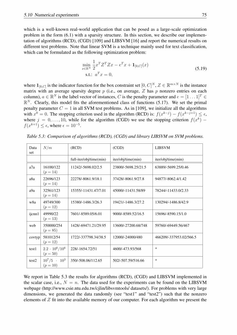
5.10 Numerical experiments 75
which is a well-known real-world application that can be posed as a large-scale optimizationproblem in the form (6.1) with a sparsity structure. In this section, we describe our implemen-tation of algorithms (RCD), (CGD) [109] and LIBSVM [16] and report the numerical results ondifferent test problems. Note that linear SVM is a technique mainly used for text classification,which can be formulated as the following optimization problem:
minx∈RN
1
2xTZTZx− eTx+ 1[0,C](x)
s.t.: aTx = 0,(5.19)
where 1[0,C] is the indicator function for the box constraint set [0, C]N , Z ∈ Rm×N is the instancematrix with an average sparsity degree p (i.e., on average, Z has p nonzero entries on eachcolumn), a ∈ RN is the label vector of instances, C is the penalty parameter and e = [1 . . . 1]T ∈RN . Clearly, this model fits the aforementioned class of functions (5.17). We set the primalpenalty parameter C = 1 in all SVM test problems. As in [109], we initialize all the algorithmswith x0 = 0. The stopping criterion used in the algorithm (RCD) is: f(xk−j) − f(xk−j+1) ≤ ϵ,where j = 0, . . . , 10, while for the algorithm (CGD) we use the stopping criterion f(xk) −f(xk+1) ≤ ϵ, where ϵ = 10−5.
Table 5.3: Comparison of algorithms (RCD), (CGD) and library LIBSVM on SVM problems.
Dataset
N/m (RCD) (CGD) LIBSVM
full-iter/obj/time(min) iter/obj/time(min) iter/obj/time(min)
a7a 16100/122(p = 14)
11242/-5698.02/2.5 23800/-5698.25/21.5 63889/-5699.25/0.46
a8a 22696/123(p = 14)
22278/-8061.9/18.1 37428/-8061.9/27.8 94877/-8062.4/1.42
a9a 32561/123(p = 14)
15355/-11431.47/7.01 45000/-11431.58/89 78244/-11433.0/2.33
w8a 49749/300(p = 12)
15380/-1486.3/26.3 19421/-1486.3/27.2 130294/-1486.8/42.9
ijcnn1 49990/22(p = 13)
7601/-8589.05/6.01 9000/-8589.52/16.5 15696/-8590.15/1.0
web 350000/254(p = 85)
1428/-69471.21/29.95 13600/-27200.68/748 59760/-69449.56/467
covtyp 581012/54(p = 12)
1722/-337798.34/38.5 12000/-24000/480 466209/-337953.02/566.5
test1 2.2 · 106/106(p = 50)
228/-1654.72/51 4600/-473.93/568 *
test2 107/5 · 103
(p = 10)350/-508.06/112.65 502/-507.59/516.66 *
We report in Table 5.3 the results for algorithms (RCD), (CGD) and LIBSVM implemented inthe scalar case, i.e., N = n. The data used for the experiments can be found on the LIBSVMwebpage (http://www.csie.ntu.edu.tw/cjlin/libsvmtools/ datasets/). For problems with very largedimensions, we generated the data randomly (see “test1” and “test2”) such that the nonzeroelements of Z fit into the available memory of our computer. For each algorithm we present the
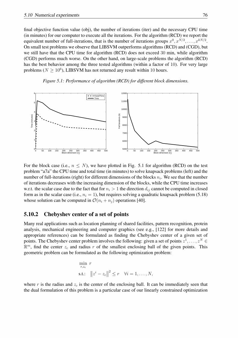
5.10 Numerical experiments 76
final objective function value (obj), the number of iterations (iter) and the necessary CPU time(in minutes) for our computer to execute all the iterations. For the algorithm (RCD) we report theequivalent number of full-iterations, that is the number of iterations groups x0, xN/2, . . . , xkN/2.On small test problems we observe that LIBSVM outperforms algorithms (RCD) and (CGD), butwe still have that the CPU time for algorithm (RCD) does not exceed 30 min, while algorithm(CGD) performs much worse. On the other hand, on large-scale problems the algorithm (RCD)has the best behavior among the three tested algorithms (within a factor of 10). For very largeproblems (N ≥ 106), LIBSVM has not returned any result within 10 hours.
Figure 5.1: Performance of algorithm (RCD) for different block dimensions.
0 50 100 150 200 250 300 350 400 450 5000
1
2
3
4
5
6
Block dimension (ni)
Tim
e (m
inut
es)
KiwielTimeTime
0 50 100 150 200 250 300 350 400 450 5005000
6000
7000
8000
9000
10000
11000
12000
Block dimension (ni)
Ful
l Ite
ratio
ns (
k)
For the block case (i.e., n ≤ N ), we have plotted in Fig. 5.1 for algorithm (RCD) on the testproblem “a7a” the CPU time and total time (in minutes) to solve knapsack problems (left) and thenumber of full-iterations (right) for different dimensions of the blocks ni. We see that the numberof iterations decreases with the increasing dimension of the blocks, while the CPU time increasesw.r.t. the scalar case due to the fact that for ni > 1 the direction dij cannot be computed in closedform as in the scalar case (i.e., ni = 1), but requires solving a quadratic knapsack problem (5.18)whose solution can be computed in O(ni + nj) operations [40].
5.10.2 Chebyshev center of a set of pointsMany real applications such as location planning of shared facilities, pattern recognition, proteinanalysis, mechanical engineering and computer graphics (see e.g., [122] for more details andappropriate references) can be formulated as finding the Chebyshev center of a given set ofpoints. The Chebyshev center problem involves the following: given a set of points z1, . . . , zN ∈Rm, find the center zc and radius r of the smallest enclosing ball of the given points. Thisgeometric problem can be formulated as the following optimization problem:
minr,zc
r
s.t.:∥∥zi − zc∥∥2 ≤ r ∀i = 1, . . . , N,
where r is the radius and zc is the center of the enclosing ball. It can be immediately seen thatthe dual formulation of this problem is a particular case of our linearly constrained optimization
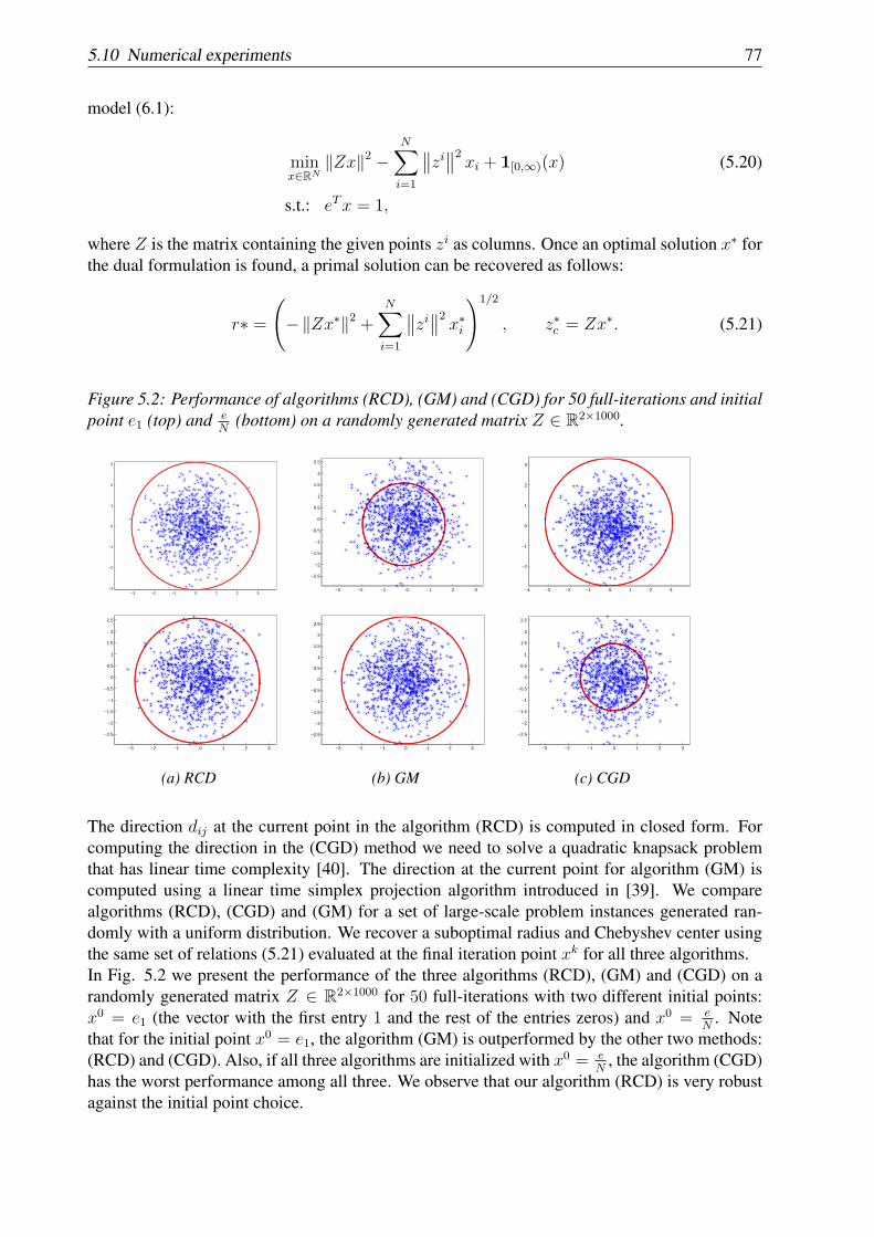
5.10 Numerical experiments 77
model (6.1):
minx∈RN
∥Zx∥2 −N∑i=1
∥∥zi∥∥2 xi + 1[0,∞)(x) (5.20)
s.t.: eTx = 1,
where Z is the matrix containing the given points zi as columns. Once an optimal solution x∗ forthe dual formulation is found, a primal solution can be recovered as follows:
r∗ =
(−∥Zx∗∥2 +
N∑i=1
∥∥zi∥∥2 x∗i)1/2
, z∗c = Zx∗. (5.21)
Figure 5.2: Performance of algorithms (RCD), (GM) and (CGD) for 50 full-iterations and initialpoint e1 (top) and e
N(bottom) on a randomly generated matrix Z ∈ R2×1000.
−3 −2 −1 0 1 2 3−3
−2
−1
0
1
2
3
−3 −2 −1 0 1 2 3
−2.5
−2
−1.5
−1
−0.5
0
0.5
1
1.5
2
2.5
(a) RCD
−3 −2 −1 0 1 2 3
−2.5
−2
−1.5
−1
−0.5
0
0.5
1
1.5
2
2.5
−3 −2 −1 0 1 2 3
−2.5
−2
−1.5
−1
−0.5
0
0.5
1
1.5
2
2.5
(b) GM
−4 −3 −2 −1 0 1 2 3
−2
−1
0
1
2
3
−3 −2 −1 0 1 2 3
−2.5
−2
−1.5
−1
−0.5
0
0.5
1
1.5
2
2.5
(c) CGD
The direction dij at the current point in the algorithm (RCD) is computed in closed form. Forcomputing the direction in the (CGD) method we need to solve a quadratic knapsack problemthat has linear time complexity [40]. The direction at the current point for algorithm (GM) iscomputed using a linear time simplex projection algorithm introduced in [39]. We comparealgorithms (RCD), (CGD) and (GM) for a set of large-scale problem instances generated ran-domly with a uniform distribution. We recover a suboptimal radius and Chebyshev center usingthe same set of relations (5.21) evaluated at the final iteration point xk for all three algorithms.In Fig. 5.2 we present the performance of the three algorithms (RCD), (GM) and (CGD) on arandomly generated matrix Z ∈ R2×1000 for 50 full-iterations with two different initial points:x0 = e1 (the vector with the first entry 1 and the rest of the entries zeros) and x0 = e
N. Note
that for the initial point x0 = e1, the algorithm (GM) is outperformed by the other two methods:(RCD) and (CGD). Also, if all three algorithms are initialized with x0 = e
N, the algorithm (CGD)
has the worst performance among all three. We observe that our algorithm (RCD) is very robustagainst the initial point choice.
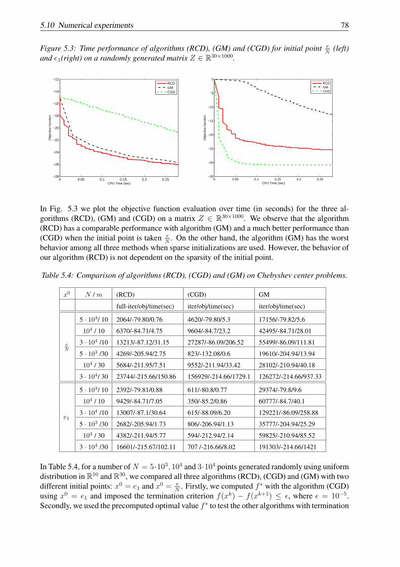
5.10 Numerical experiments 78
Figure 5.3: Time performance of algorithms (RCD), (GM) and (CGD) for initial point eN
(left)and e1(right) on a randomly generated matrix Z ∈ R30×1000.
0 0.05 0.1 0.15 0.2 0.25−28
−26
−24
−22
−20
−18
−16
−14
−12
CPU Time (sec)
Obj
ectiv
e fu
nctio
n
RCDGMCGD
0 0.05 0.1 0.15 0.2 0.25−35
−30
−25
−20
−15
−10
−5
0
CPU Time (sec)
Obj
ectiv
e fu
nctio
n
RCDGMCGD
In Fig. 5.3 we plot the objective function evaluation over time (in seconds) for the three al-gorithms (RCD), (GM) and (CGD) on a matrix Z ∈ R30×1000. We observe that the algorithm(RCD) has a comparable performance with algorithm (GM) and a much better performance than(CGD) when the initial point is taken e
N. On the other hand, the algorithm (GM) has the worst
behavior among all three methods when sparse initializations are used. However, the behavior ofour algorithm (RCD) is not dependent on the sparsity of the initial point.
Table 5.4: Comparison of algorithms (RCD), (CGD) and (GM) on Chebyshev center problems.
x0 N / m (RCD) (CGD) GM
full-iter/obj/time(sec) iter/obj/time(sec) iter/obj/time(sec)
eN
5 · 103/ 10 2064/-79.80/0.76 4620/-79.80/5.3 17156/-79.82/5.6
104 / 10 6370/-84.71/4.75 9604/-84.7/23.2 42495/-84.71/28.01
3 · 104 /10 13213/-87.12/31.15 27287/-86.09/206.52 55499/-86.09/111.81
5 · 103 /30 4269/-205.94/2.75 823/-132.08/0.6 19610/-204.94/13.94
104 / 30 5684/-211.95/7.51 9552/-211.94/33.42 28102/-210.94/40.18
3 · 104/ 30 23744/-215.66/150.86 156929/-214.66/1729.1 126272/-214.66/937.33
e1
5 · 103/ 10 2392/-79.81/0.88 611/-80.8/0.77 29374/-79.8/9.6
104 / 10 9429/-84.71/7.05 350/-85.2/0.86 60777/-84.7/40.1
3 · 104 /10 13007/-87.1/30.64 615/-88.09/6.20 129221/-86.09/258.88
5 · 103 /30 2682/-205.94/1.73 806/-206.94/1.13 35777/-204.94/25.29
104 / 30 4382/-211.94/5.77 594/-212.94/2.14 59825/-210.94/85.52
3 · 104 /30 16601/-215.67/102.11 707 /-216.66/8.02 191303/-214.66/1421
In Table 5.4, for a number ofN = 5·103, 104 and 3·104 points generated randomly using uniformdistribution in R10 and R30, we compared all three algorithms (RCD), (CGD) and (GM) with twodifferent initial points: x0 = e1 and x0 = e
N. Firstly, we computed f ∗ with the algorithm (CGD)
using x0 = e1 and imposed the termination criterion f(xk) − f(xk+1) ≤ ϵ, where ϵ = 10−5.Secondly, we used the precomputed optimal value f ∗ to test the other algorithms with termination
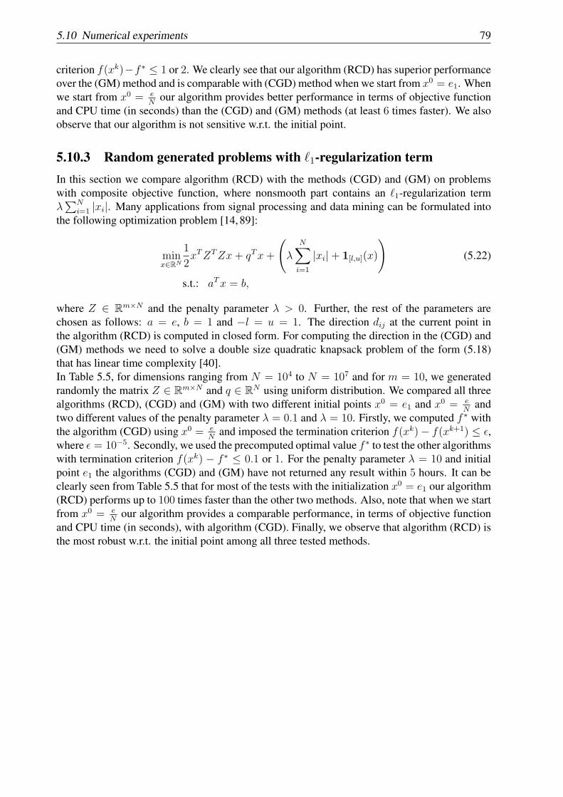
5.10 Numerical experiments 79
criterion f(xk)−f ∗ ≤ 1 or 2. We clearly see that our algorithm (RCD) has superior performanceover the (GM) method and is comparable with (CGD) method when we start from x0 = e1. Whenwe start from x0 = e
Nour algorithm provides better performance in terms of objective function
and CPU time (in seconds) than the (CGD) and (GM) methods (at least 6 times faster). We alsoobserve that our algorithm is not sensitive w.r.t. the initial point.
5.10.3 Random generated problems with ℓ1-regularization termIn this section we compare algorithm (RCD) with the methods (CGD) and (GM) on problemswith composite objective function, where nonsmooth part contains an ℓ1-regularization termλ∑N
i=1 |xi|. Many applications from signal processing and data mining can be formulated intothe following optimization problem [14, 89]:
minx∈RN
1
2xTZTZx+ qTx+
(λ
N∑i=1
|xi|+ 1[l,u](x)
)(5.22)
s.t.: aTx = b,
where Z ∈ Rm×N and the penalty parameter λ > 0. Further, the rest of the parameters arechosen as follows: a = e, b = 1 and −l = u = 1. The direction dij at the current point inthe algorithm (RCD) is computed in closed form. For computing the direction in the (CGD) and(GM) methods we need to solve a double size quadratic knapsack problem of the form (5.18)that has linear time complexity [40].In Table 5.5, for dimensions ranging from N = 104 to N = 107 and for m = 10, we generatedrandomly the matrix Z ∈ Rm×N and q ∈ RN using uniform distribution. We compared all threealgorithms (RCD), (CGD) and (GM) with two different initial points x0 = e1 and x0 = e
Nand
two different values of the penalty parameter λ = 0.1 and λ = 10. Firstly, we computed f ∗ withthe algorithm (CGD) using x0 = e
Nand imposed the termination criterion f(xk)− f(xk+1) ≤ ϵ,
where ϵ = 10−5. Secondly, we used the precomputed optimal value f ∗ to test the other algorithmswith termination criterion f(xk) − f ∗ ≤ 0.1 or 1. For the penalty parameter λ = 10 and initialpoint e1 the algorithms (CGD) and (GM) have not returned any result within 5 hours. It can beclearly seen from Table 5.5 that for most of the tests with the initialization x0 = e1 our algorithm(RCD) performs up to 100 times faster than the other two methods. Also, note that when we startfrom x0 = e
Nour algorithm provides a comparable performance, in terms of objective function
and CPU time (in seconds), with algorithm (CGD). Finally, we observe that algorithm (RCD) isthe most robust w.r.t. the initial point among all three tested methods.
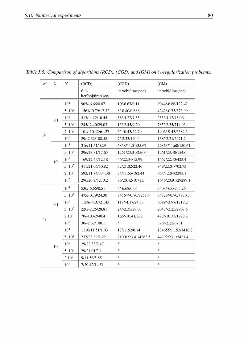
5.10 Numerical experiments 80
Table 5.5: Comparison of algorithms (RCD), (CGD) and (GM) on ℓ1-regularization problems.
x0 λ N (RCD) (CGD) (GM)
full-iter/obj/time(sec)
iter/obj/time(sec) iter/obj/time(sec)
eN
0.1
104 905/-6.66/0.87 10/-6.67/0.11 9044/-6.66/122.42
5 ·104 1561/-0.79/12.32 8/-0.80/0.686 4242/-0.75/373.99
105 513/-4.12/10.45 58/-4.22/7.55 253/-4.12/45.06
5 ·105 245/-2.40/29.03 13/-2.45/9.20 785/-2.35/714.93
2 ·106 101/-10.42/61.27 6/-10.43/22.79 1906/-9.43/6582.5
107 29/-2.32/108.58 7/-2.33/140.4 138/-2.21/2471.2
10
104 316/11.51/0.29 5858/11.51/35.67 22863/11.60/150.61
5 ·104 296/23.31/17.65 1261/23.31/256.6 1261/23.40/154.6
105 169/22.43/12.18 46/22.34/15.99 1467/22.43/423.4
5 ·105 411/21.06/50.82 37/21.02/22.46 849/22.01/702.73
2 ·106 592/11.84/334.30 74/11.55/182.44 664/12.04/2293.1
107 296/20.9/5270.2 76/20.42/1071.5 1646/20.91/29289.1
e1
0.1
104 536/-6.66/0.51 4/-6.68/0.05 3408/-6.66/35.26
5 ·104 475/-0.79/24.30 84564/-0.70/7251.4 54325/-0.70/4970.7
105 1158/-4.07/21.43 118/-4.17/24.83 6699/-3.97/1718.2
5 ·105 226/-2.25/28.81 24/-2.35/29.03 2047/-2.25/2907.5
2·106 70/-10.42/40.4 166/-10.41/632 428/-10.33/1728.3
107 30/-2.32/100.1 * 376/-2.22/6731
10
104 1110/11.51/1.03 17/11.52/0.14 184655/11.52/1416.8
5 ·104 237/23.39/1.22 21001/23.41/4263.5 44392/23.1/5421.4
105 29/22.33/2.47 * *
5 ·105 29/21.01/3.1 * *
2·106 9/11.56/5.85 * *
107 7/20.42/14.51 * *
Chapter 6
Random coordinate descent methods fornonconvex composite optimization
In this chapter we analyze several new methods for solving nonconvex optimization problemswith the objective function formed as a sum of two terms: one is nonconvex and smooth, andanother is convex but simple and its structure is known. Further, we consider both cases: un-constrained and linearly constrained nonconvex problems. For optimization problems of theabove structure, we propose random coordinate descent algorithms and analyze their conver-gence properties. For the general case, when the objective function is nonconvex and compositewe prove asymptotic convergence for the sequences generated by our algorithms to stationarypoints and sublinear rate of convergence in expectation for some optimality measure. Addi-tionally, if the objective function satisfies an error bound condition we derive a local linearrate of convergence for the expected values of the objective function. We also present extensivenumerical experiments for evaluating the performance of our algorithms in comparison withstate-of-the-art methods. This chapter is based on paper [84, 85].
6.1 IntroductionCoordinate descent methods are among the first algorithms used for solving general minimiza-tion problems and one of the most successful in the large-scale optimization field [8]. Roughlyspeaking, coordinate descent methods are based on the strategy of updating one (block) coordi-nate of the vector of variables per iteration using some index selection procedure (e.g. cyclic,greedy, random). For example, the nonlinear Gauss-Seidel method consists in the exact min-imization of the objective function over one coordinate of the decision variable, chosen in acyclic fashion, while the others remain fixed at the current point. These strategies often reducesdrastically the iteration complexity and memory requirements, making these methods simpleand scalable. There exist numerous papers dealing with the convergence analysis of this typeof methods [2, 5, 49, 88, 108], which confirm the difficulties encountered in proving the con-vergence for nonconvex and nonsmooth objective functions. For instance, regarding coordinateminimization of nonconvex functions, Powell [88] provided some examples of differentiablefunctions whose properties lead the algorithm to a closed loop. Also, proving convergence ofcoordinate descent for minimization of nondifferentiable objective functions is challenging [2].However, for nonconvex and nonsmooth objective functions with certain structure (e.g. compos-ite objective functions) there are available convergence results for coordinate descent methodsbased on greedy index selection [5, 49, 108]. Recently, Nesterov [76] derived complexity results
81
6.1 Introduction 82
for random coordinate gradient descent methods for solving smooth and convex minimizationproblems. In [93] the authors generalized Nesterov’ results to convex problems with compositeobjective functions. Extensive complexity analysis of coordinate gradient descent methods forsolving linearly constrained optimization problems with convex (composite) objective functioncan be found in previous chapters, but also in a recent paper [5].In this chapter we also consider large-scale nonconvex optimization problems with the objectivefunction formed as a sum of two terms: one is nonconvex, smooth and given by a black-boxoracle, and another is convex but simple and its structure is known. Further, we analyze un-constrained but also singly linearly constrained nonconvex problems. We also suppose that thedimension of the problem is so large that traditional optimization methods cannot be directlyemployed since basic operations, such as the updating of the gradient, are too computationallyexpensive. These type of problems arise in many fields such as data analysis (speech denois-ing, classification, text mining) [11, 18], systems and control theory (optimal control, stabilityof positive bilinear and linear switched systems, simultaneous stabilization of linear systems,pole assignment by static output feedback) [3, 26, 39, 61, 83, 104], machine learning [18, 111],traffic equilibrium and network flow problems [23], truss topology design [42]. The goal of thischapter is to analyze several new random coordinate gradient descent methods suited for large-scale nonconvex problems with composite objective function. Up to our knowledge, there isno convergence analysis of random coordinate descent algorithms for solving nonconvex nons-mooth optimization problems. For the coordinate descent algorithm designed to minimize un-constrained composite nonconvex objective functions we prove asymptotic convergence of thegenerated sequence to stationary points and sublinear rate of convergence in expectation for someoptimality measure. Additionally, if the objective function satisfies an error bound condition, alocal linear rate of convergence for expected values of the objective function is obtained. Wealso provide convergence analysis for a coordinate descent method designed for solving singlylinearly constrained nonconvex problems and obtain similar results as in the unconstrained case.Note that our analysis is very different from the convex case given in the previous chapters(see also [68,70,76,93]) and is based on the notion of optimality measure and a supermartingaleconvergence theorem. On the other hand, compared to other coordinate descent methods for non-convex problems our algorithms offer some important advantages, e.g. due to the randomizationour algorithms are simpler, are adequate for modern computational architectures and they leadto more robust output. We also present the results of preliminary computational experiments,which confirm the superiority of our methods compared with other algorithms for large-scalenonconvex optimization.The contribution of the chapter can be summarized as follows: For unconstrained problems wepropose an 1-coordinate descent method (1-CD), that involves at each iteration the solution anoptimization subproblem only with respect to one (block) variable while keeping all others fixed.We show that usually this solution can be computed in closed form; For linearly constrainedcase we propose a 2-coordinate descent method (2-CD), that involves at each iteration the solu-tion of a subproblem depending on two (block) variables while keeping all other variables fixed.We show that in most of the cases this solution can be found in linear time; For each of thealgorithms we introduce some optimality measure and devise a convergence analysis using thisframework. In particular, for both algorithms, (1-CD) and (2-CD), we establish asymptotic con-vergence of the generated sequences to stationary points and sublinear rate of convergence forthe expected values of the corresponding optimality measures; If the objective function satisfiesan error bound condition a local linear rate of convergence for expected values of the objectivefunction is proved.The structure of the chapter is as follows. In Section 6.2 we introduce an 1-random coordinate
6.2 Unconstrained minimization of composite objective functions 83
descent algorithm for unconstrained minimization of nonconvex composite functions. Further weanalyze the convergence properties of the algorithm under standard assumptions and under theerror bound assumption we obtain linear convergence rate for the expected values of objectivefunction. In Section 6.3 we derive a 2-coordinate descent method for solving singly linearlyconstrained nonconvex problems and analyze its convergence. In Section 6.4 we report numericalresults on large-scale eigenvalue complementarity problems, which is an important applicationin control theory.
6.2 Unconstrained minimization of composite objective func-tions
In this section we analyze a variant of random block coordinate gradient descent method, whichwe call 1-coordinate descent method (1-CD), for solving large-scale unconstrained nonconvexproblems with composite objective function. The method involves at each iteration the solutionof an optimization subproblem only with respect to one (block) variable while keeping all othervariables fixed. After discussing several necessary mathematical preliminaries, we introduce anoptimality measure, which will be the basis for the construction and analysis of Algorithm (1-CD). We establish asymptotic convergence of the sequence generated by Algorithm (1-CD) toa stationary point and then we show sublinear rate of convergence in expectation for the cor-responding optimality measure. For some well-known particular cases of nonconvex objectivefunctions arising frequently in applications, the complexity per iteration of our Algorithm (1-CD)is of order O(ni).
6.2.1 Problem formulationWe consider the space Rn composed by column vectors. For x, y ∈ Rn we denote the scalarproduct by ⟨x, y⟩ = xTy and ∥x∥ = (xTx)1/2. We use the same notation ⟨·, ·⟩ and ∥·∥ for scalarproducts and norms in spaces of different dimensions. For some norm ∥·∥α in Rn, its dual normis defined by ∥y∥∗α = max∥x∥α=1⟨y, x⟩. We consider the following decomposition of the variabledimension: n =
∑Ni=1 ni. Also, we denote a block decomposition of n × n identity matrix by
In = [U1 . . . UN ], where Ui ∈ Rn×ni . For brevity we use the following notation: for all x ∈ Rn
and i, j = 1, . . . , N , we denote:
xi = UTi x ∈ Rni , ∇if(x) = UT
i ∇f(x) ∈ Rni
xij =[xTi x
Tj
]T ∈ Rni+nj , ∇ijf(x) =[∇if(x)
T ∇jf(x)T]T ∈ Rni+nj .
The problem of interest in this section is the unconstrained nonconvex minimization problemwith composite objective function:
F ∗ = minx∈Rn
F (x) (:= f(x) + h(x)) , (6.1)
where the function f is smooth and h is a convex, separable, nonsmooth function. Since h isnonsmooth, then for any x ∈ dom(h) we denote by ∂h(x) the subdifferential (set of subgradi-ents) of h at x. The smooth and nonsmooth components in the objective function of (6.1) satisfythe following assumptions:
6.2 Unconstrained minimization of composite objective functions 84
Assumption 6.2.1 (i) The function f has block coordinate Lipschitz continuous gradient, i.e.there are constants Li > 0 such that:
∥∇if(x+ Uisi)−∇if(x)∥ ≤ Li ∥si∥ ∀si ∈ Rni , x ∈ Rn, i = 1, . . . , N.
(ii) The function h is proper, convex, continuous and block separable:
h(x) =N∑i=1
hi(xi) ∀x ∈ Rn,
where the functions hi : Rni → R are convex for all i = 1, . . . , N .
These assumptions are typical for the coordinate descent framework as the reader can find similarvariants in [70, 76, 93, 108]. An immediate consequence of Assumption 6.2.1 (i) is the followingwell-known inequality [75]:
|f(x+ Uisi)− f(x)− ⟨∇if(x), si⟩| ≤Li
2∥si∥2 ∀si ∈ Rni , x ∈ Rn. (6.2)
Based on this quadratic approximation of function f we get the inequality:
F (x+ Uisi) ≤ f(x) + ⟨∇if(x), si⟩+Li
2∥si∥2 + h(x+ Uisi) ∀si ∈ Rni , x ∈ Rn. (6.3)
Given local Lipschitz constants Li > 0 for i = 1, . . . , N , we define the vector L =[L1 . . . LN ]
T ∈ RN , the diagonal matrix DL = diag(L1In1 , . . . , LNInN) ∈ Rn×n and the fol-
lowing pair of dual norms:
∥x∥L =
(N∑i=1
Li ∥xi∥2)1/2
∀x ∈ Rn, ∥y∥∗L =
(N∑i=1
L−1i ∥yi∥
2
)1/2
∀y ∈ Rn.
Using Assumption 6.2.1, we can state the first order necessary optimality conditions for the non-convex optimization problem (6.1): if x∗ ∈ Rn is a local minimum for (6.1), then the followingrelation holds
0 ∈ ∇f(x∗) + ∂h(x∗).
Any vector x∗ satisfying this relation is called a stationary point for nonconvex problem (6.1).
6.2.2 An 1-random coordinate descent algorithmWe analyze a variant of random coordinate descent method suitable for solving large-scale non-convex problems in the form (6.1). Let i ∈ 1, . . . , N be a random variable and pik = Pr(i = ik)be its probability distribution. Given a point x, one block is chosen randomly with respect to theprobability distribution pi and the quadratic model (6.3) derived from the composite objectivefunction is minimized with respect to this block of coordinates (see also [76, 93]). Our methodhas the following iteration: given an initial point x0, then for all k ≥ 0
Algorithm (1-CD)1. Choose randomly a block of coordinates ik with probability pik2. Set xk+1 = xk + Uikdik ,
6.2 Unconstrained minimization of composite objective functions 85
where the direction dik is chosen as follows:
dik = arg minsik∈R
nik
f(xk) + ⟨∇ikf(xk), sik⟩+
Lik
2∥sik∥
2 + h(xk + Uiksik). (6.4)
Note that the direction dik is a minimizer of the quadratic approximation model given in (6.3).Further, from Assumption 6.2.1 (ii) we see that h(xk + Uiksik) = hik(x
kik+ sik) +
∑i=ik
hi(xki )
and thus for computing dik we only need to know the function hik(·). An important propertyof our algorithm is that for certain particular cases of function h, the iteration complexity ofAlgorithm (1-CD) is very low. In particular, for certain simple functions h, very often met inmany applications from signal processing, machine learning, optimal control, the direction dikcan be computed in closed form, e.g.:
(I) For some l, u ∈ Rn, with l ≤ u, we consider the box indicator function
h(x) =
0 if l ≤ x ≤ u
∞ otherwise.(6.5)
In this case the direction dik has the explicit expression:
dik =
[xkik −
1
Lik
∇ikf(xk)
][lik , uik
]
∀ik = 1, . . . , N,
where [x][l, u] is the orthogonal projection of vector x on box set [l, u].
(II) Given a nonnegative scalar β ∈ R+, we consider the ℓ1-regularization function defined bythe 1-norm
h(x) = β ∥x∥1 . (6.6)
In this case, considering n = N , the direction dik has the explicit expression:
dik = sgn(tik) ·max
|tik | −
β
Lik
, 0
− xik ∀ik = 1, . . . , n,
where tik = xik − 1Lik∇ikf(x
k).
In these examples the arithmetic complexity of computing the next iterate xk+1, once∇ikf(xk) is
known, is of orderO(nik). The reader can find other favorable examples of nonsmooth functionsh which preserve the low iteration complexity of Algorithm (1-CD) (see also [93, 108] for otherexamples). Note that other (coordinate descent) methods designed for solving nonconvex prob-lems have complexity per iteration at least of order O(n) [108]. But Algorithm (1-CD) offersalso other important advantages, e.g. due to the randomization the algorithm leads to more ro-bust output and is adequate for modern computational architectures (e.g distributed and parallelarchitectures) [61, 94].We assume that the sequence of random variables i0, . . . , ik are i.i.d. In the sequel, we use thenotation ξk for the entire history of random index selection
ξk = i0, . . . , ik .
and notationϕk = E
[F (xk)
]
6.2 Unconstrained minimization of composite objective functions 86
for the expectation taken w.r.t. ξk−1. Given s, x ∈ Rn, we introduce the following function andthe associated map (operator):
ψL(s; x) = f(x) + ⟨∇f(x), s⟩+ 1
2∥s∥2L + h(x+ s),
dL(x) = arg mins∈Rn
f(x) + ⟨∇f(x), s⟩+ 1
2∥s∥2L + h(x+ s). (6.7)
Based on this map, we now introduce an optimality measure which will be the basis for theanalysis of Algorithm (1-CD):
M1(x, L) = ∥DL · dL(x)∥∗L .
The map M1(x, L) is an optimality measure for optimization problem (6.1) in the sense that it ispositive for all nonstationary points and zero for stationary points (see Lemma 6.2.2 below):
Lemma 6.2.2 For any given vector L ∈ RN with positive entries, a vector x∗ ∈ Rn is a station-ary point for problem (6.1) if and only if the value M1(x
∗, L) = 0.
Proof : : Based on the optimality conditions of subproblem (6.7), it can be easily shown that ifM1(x
∗, L) = 0, then x∗ is a stationary point for the original problem (6.1). We prove the converseimplication by contradiction. Assume that x∗ is a stationary point for (6.1) andM1(x
∗, L) > 0. Itfollows that dL(x
∗) is a nonzero solution of subproblem (6.7). Then, there exist the subgradientsg(x∗) ∈ ∂h(x∗) and g(x∗ + dL(x
∗)) ∈ ∂h(x∗ + dL(x∗)) such that the optimality conditions for
optimization problems (6.1) and (6.7) can be written as:∇f(x∗) + g(x∗) = 0
∇f(x∗) +DLdL(x∗) + g(x∗ + dL(x
∗)) = 0.
Taking the difference of the two relations above and considering the inner product with dL(x∗) =
0 on both sides of the equation, we get:
∥dL(x∗)∥2L + ⟨g(x∗ + dL(x
∗))− g(x∗), dL(x∗)⟩ = 0.
From convexity of the function h we see that both terms in the above sum are nonnegative andthus dL(x
∗) = 0, which contradicts our hypothesis. In conclusion M1(x∗, L) = 0. 2
Note that ψL(s; x) is an 1-strongly convex function in the variable s w.r.t. norm ∥·∥L and thusdL(x) is unique and the following inequality holds:
ψL(s; x) ≥ ψL(dL(x);x) +1
2∥dL(x)− s∥2L ∀x, s ∈ Rn. (6.8)
6.2.3 ConvergenceIn this section, we analyze the convergence properties of Algorithm (1-CD). Firstly, we provethe asymptotic convergence of the sequence generated by Algorithm (1-CD) to stationary points.For proving the asymptotic convergence we use the following supermartingale convergence resultdue to Robbins and Siegmund (see [87, Lemma 11 on page 50]):
6.2 Unconstrained minimization of composite objective functions 87
Lemma 6.2.3 Let vk, uk and αk be three sequences of nonnegative random variables such that
E[vk+1|Fk] ≤ (1 + αk)vk − uk ∀k ≥ 0 a.s. and∞∑k=0
αk <∞ a.s.,
where Fk denotes the collections v0, . . . , vk, u0, . . . , uk, α0, . . . , αk. Then, we have limk→∞ vk =v for a random variable v ≥ 0 a.s. and
∑∞k=0 uk <∞ a.s.
In the next lemma we prove that Algorithm (1-CD) is a descent method, i.e. the objective functionis nonincreasing along the iterations:
Lemma 6.2.4 Let xk be the sequence generated by Algorithm (1-CD) under Assumption 6.2.1.Then, the following relation holds:
F (xk+1) ≤ F (xk)− Lik
2∥dik∥
2 ∀k ≥ 0. (6.9)
Proof : : From the optimality conditions of subproblem (6.4) we have that there exists a subgra-dient g(xkik + dik) ∈ ∂hik(xkik + dik) such that:
∇ikf(xk) + Likdik + g(xkik + dik) = 0.
On the other hand, since the function hik is convex, according to Assumption 6.2.1 (ii), thefollowing inequality holds:
hik(xkik+ dik)− hik(xkik) ≤ ⟨g(x
kik+ dik), dik⟩
Applying the previous two inequalities in (6.3) and using the separability of the function h,according to Assumption 6.2.1 (ii), we have:
F (xk+1) ≤ F (xk) + ⟨∇ikf(xk), dik⟩+
Lik
2∥dik∥
2 + hik(xkik+ dik)− hik(xkik)
≤ F (xk) + ⟨∇ikf(xk), dik⟩+
Lik
2∥dik∥
2 + ⟨g(xkik + dik), dik⟩
≤ F (xk)− Lik
2∥dik∥
2 .
2
Using Lemma 6.2.4, we state the following result regarding the asymptotic convergence of Al-gorithm (1-CD).
Theorem 6.2.5 If Assumption 6.2.1 holds for the composite objective function F of problem(6.1) and the sequence xk is generated by Algorithm (1-CD) using the uniform distribution, thenthe following statements are valid:
(i) The sequence of random variables M1(xk, L) converges to 0 a.s. and the sequence F (xk)
converges to a random variable F a.s.
(ii) Any accumulation point of the sequence xk is a stationary point for optimization prob-lem (6.1).
6.2 Unconstrained minimization of composite objective functions 88
Proof : (i) From Lemma 6.2.4 we get:
F (xk+1)− F ∗ ≤ F (xk)− F ∗ − Lik
2∥dik∥
2 ∀k ≥ 0.
We now take the expectation conditioned on ξk−1 and note that ik is independent on the pastξk−1, while xk is fully determined by ξk−1 and thus:
E[F (xk+1)− F ∗| ξk−1
]≤ F (xk)− F ∗ − 1
2E[Lik · ∥dik∥
2 | ξk−1]
≤ F (xk)− F ∗ − 1
2N
∥∥dL(xk)∥∥2L .Using the supermartingale convergence theorem given in Lemma 6.2.3 in the previous inequality,we can ensure that
limk→∞
F (xk)− F ∗ = θ a.s.
for a random variable θ ≥ 0 and thus F = θ + F ∗. Further, due to almost sure convergence ofsequence F (xk), it can be easily seen that lim
k→∞F (xk) − F (xk+1) = 0 a.s. From xk+1 − xk =
Uikdik and Lemma 6.2.4 we have:
Lik
2∥dik∥
2 =Lik
2
∥∥xk+1 − xk∥∥2 ≤ F (xk)− F (xk+1) ∀k ≥ 0,
which implies that
limk→∞
∥∥xk+1 − xk∥∥ = 0 and lim
k→∞∥dik∥ = 0 a.s.
As ∥dik∥ → 0 a.s., we can conclude that the random variable E[∥dik∥ |ξk−1]→ 0 a.s. or equiva-lently M1(x
k, L)→ 0 a.s.(ii) For brevity we assume that the entire sequence xk generated by Algorithm (1-CD) is con-vergent. Let x be the limit point of the sequence xk. From the first part of the theorem we haveproved that the sequence of random variables dL(xk) converges to 0 a.s. Using the definition ofdL(x
k) we have:
f(xk) + ⟨∇f(xk), dL(xk)⟩+1
2
∥∥dL(xk)∥∥2L + h(xk + dL(xk))
≤ f(xk) + ⟨∇f(xk), s⟩+ 1
2∥s∥2L + h(xk + s) ∀s ∈ Rn,
and taking the limit k →∞ and using Assumption 6.2.1 (ii) we get:
F (x) ≤ f(x) + ⟨∇f(x), s⟩+ 1
2∥s∥2L + h(x+ s) ∀s ∈ Rn.
This shows that dL(x) = 0 is the minimum in subproblem (6.7) for x = x and thusM1(x, L) = 0.From Lemma 6.2.2 we conclude that x is a stationary point for optimization problem (6.1). 2
The next theorem proves the convergence rate of the optimality measure M1(xk, L) towards 0 in
expectation.
6.2 Unconstrained minimization of composite objective functions 89
Theorem 6.2.6 Let F satisfy Assumption 6.2.1. Then, the Algorithm (1-CD) based on the uni-form distribution generates a sequence xk satisfying the following convergence rate for the ex-pected values of the optimality measure:
min0≤l≤k
E[(M1(x
l, L))2] ≤ 2N (F (x0)− F ∗)
k + 1∀k ≥ 0.
Proof : : For simplicity of the exposition we use the following notation: given the current iteratex, denote x+ = x + Uidi the next iterate, where direction di is given by (6.4) for some randomchosen index i w.r.t. uniform distribution. For brevity, we also adapt the notation of expectationupon the entire history, i.e. (ϕ, ϕ+, ξ) instead of (ϕk, ϕk+1, ξk−1). From Assumption 6.2.1 andinequality (6.3) we have:
F (x+) ≤ f(x) + ⟨∇if(x), di⟩+Li
2∥di∥2 + hi(xi + di) +
∑j =i
hj(xj)
Now we take the expectation conditioned on ξ:
E[F (x+)| ξ] ≤E[f(x)+⟨∇if(x), di⟩+
Li
2∥di∥2 + hi(xi + di)+
∑j =i
hj(xj)| ξ]
≤ f(x) +1
N
[⟨∇f(x), dL(x)⟩+
1
2∥dL(x)∥2L + h(x+ dL(x)) + (N − 1)h(x)
].
After arranging the above expression we get:
E[F (x+)| ξ] ≤(1− 1
N
)F (x) +
1
NψL(dL(x);x). (6.10)
Now, taking the expectation in (6.10) w.r.t. ξ we obtain:
ϕ+ ≤(1− 1
N
)ϕ+ E
[1
NψL(dL(x);x)
], (6.11)
and then using the 1−strong convexity property of ψL we get:
ϕ− ϕ+ ≥ ϕ−(1− 1
N
)ϕ− 1
NE [ψL(dL(x); x)]
=1
N(E [ψL(0;x)]− E[ψL(dL(x); x)])
≥ 1
2NE[∥dL(x)∥2L
]=
1
2NE[(M1(x, L))
2]. (6.12)
Now coming back to the notation dependent on k and summing w.r.t. the entire history we have:
1
2N
k∑l=0
E[(M1(x
l, L))2]≤ ϕ0 − F ∗,
which leads to the statement of the theorem. 2

6.2 Unconstrained minimization of composite objective functions 90
It is important to note that the convergence rate for the Algorithm (1-CD) given in Theorem 6.2.6is typical for the class of first order methods designed for solving nonconvex and nonsmotthoptimization problems (see e.g. [78] for more details). Note also that our convergence results aredifferent from the convex case [76, 93], since here we introduce another optimality measure andwe use supermartingale convergence theorem in the analysis. Furthermore, when the objectivefunction F is smooth and nonconvex, i.e. h = 0, the first order necessary conditions of optimalitybecome ∇f(x∗) = 0. Also, note that in this case, the optimality measure M1(x, L) is givenby: M1(x, L) = ∥∇f(x)∥∗L. An immediate consequence of Theorem 6.2.6 in this case is thefollowing result:
Lemma 6.2.7 Let h = 0 and f satisfy Assumption 6.2.1 (i). Then, in this case the Algorithm(1-CD) based on the uniform distribution generates a sequence xk satisfying the following con-vergence rate for the expected values of the norm of the gradients:
min0≤l≤k
E
[(∥∥∇f(xl)∥∥∗L
)2]≤ 2N (F (x0)− F ∗)
k + 1∀k ≥ 0.
6.2.4 Linear convergence for objective functions with error boundIn this subsection an improved rate of convergence is shown for Algorithm (1-CD) under anadditional error bound assumption. In what follows, X∗ denotes the set of stationary points ofoptimization problem (6.1), dist(x, S) = min
y∈S∥y − x∥ and the vector e = [1 . . . 1]T ∈ RN .
Assumption 6.2.8 A local error bound holds for the objective function of optimization problem(6.1), i.e. for any η ≥ F ∗ = min
x∈RnF (x) there exist τ > 0 and ϵ > 0 such that
dist(x,X∗) ≤ τM1(x, e) ∀x ∈ V,
where V = x ∈ Rn : F (x) ≤ η, M1(x, e) ≤ ϵ. Moreover, there exists ρ > 0 such that∥x∗ − y∗∥ ≥ ρ whenever x∗, y∗ ∈ X∗ with f(x∗) = f(y∗).
For example, Assumption 6.2.8 holds for composite objective functions satisfying the followingproperties (see [106, 108] for more examples):(i) f is quadratic function (even nonconvex) and h is polyhedral(ii) f is strongly convex, has Lipschitz continuous gradient and h is polyhedral.Note that the box indicator function (6.5) and ℓ1-regularization function (6.6) are polyhedralfunctions. Note also that for strongly convex functions, Assumption 6.2.8 is globally satisfied.In this section, we also assume that function f has global Lipschitz continuous gradient, i.e. thereexists a global Lipschitz constant Lf > 0 such that:
∥∇f(x)−∇f(y)∥ ≤ Lf ∥x− y∥ ∀x, y ∈ Rn.
It is well known that this property leads to the following inequality [75]:
|f(y)− f(x)− ⟨∇f(x), y − x⟩| ≤ Lf
2∥x− y∥2 ∀x, y ∈ Rn. (6.13)
For a given convex function h : Rn → R we also define the proximal map proxh(x) : Rn →Rn as proxh(x) = arg min
y∈Rn
12∥y − x∥2 + h(y). In order to analyze the convergence properties
of Algorithm (1-CD) for minimizing composite objective function which satisfies Assumption6.2.8, we require the following auxiliary result:

6.2 Unconstrained minimization of composite objective functions 91
Lemma 6.2.9 Let h : Rn → R be a convex function. Then, the map ω : R+ → R+ defined by
ω(α) =∥proxαh(x+ αd)− x∥
α,
is nonincreasing w.r.t. α for any x, d ∈ Rn.
Proof : Note that this lemma is a generalization of [12, Lemma 2.2] from the projection operatorto the “prox” operator case. We derive our proof based on the following remark (see also [12]):for given u, v ∈ Rn if ⟨v, u− v⟩ > 0, then
∥u∥∥v∥≤ ⟨u, u− v⟩⟨v, u− v⟩
. (6.14)
Let α > β > 0. Taking u = proxαh(x + αd) − x and v = proxβh(x + βd) − x, we show firstthat inequality ⟨v, u− v⟩ > 0 holds. Given a real constant c > 0, from the optimality conditionscorresponding to proximal operator we have:
x− proxch(x) ∈ ∂ch(proxch(x)).
Therefore, from the convexity of h we can derive that:
ch(z) ≥ ch(proxch(y)) + ⟨y − proxch(y), z − proxch(y)⟩ ∀y, z ∈ Rn.
Taking c = α, z = proxβh(x+ βd) and y = x+ αd we have:
⟨u, u− v⟩ ≤ α(⟨d, u− v⟩+ h(proxβh(x+ βd))− h(proxαh(x+ αd))
). (6.15)
Also, if c = β, z = proxαh(x+ αd) and y = x+ βd, then we have:
⟨v, u− v⟩ ≥ β (⟨d, u− v⟩+ h(proxh(x+ βd))− h(proxh(x+ αd))) . (6.16)
Summing these two inequalities and taking in account that α > β we get:
⟨d, u− v⟩+ h(proxh(x+ βd))− h(proxh(x+ αd)) > 0.
Therefore, replacing this expression into inequality (6.15) leads to ⟨v, u− v⟩ > 0. Finally, from(6.14),(6.15) and (6.16) we get the inequality:
∥u∥∥v∥≤ α⟨d, u− v⟩β⟨d, u− v⟩
,
and then the statement of Lemma 6.2.9 can be easily derived. 2
Using separability of h according to Assumption 6.2.1 (ii), it is easy to see that the map dL(x)satisfies:
x+ dL(x) = arg miny∈Rn
1
2
∥∥y − x+D−1L ∇f(x)
∥∥2 + N∑i=1
1
Li
hi(yi),
and in a more compact notation we have:
(dL(x))i = prox 1Li
hi(xi − 1/Li∇if(x))− xi ∀i = 1, . . . , N.
6.2 Unconstrained minimization of composite objective functions 92
Using this expression in Lemma 6.2.9, we conclude that:
∥(de(x))i∥ ≤ max1, Li · ∥(dL(x))i∥ ∀i = 1, . . . , N (6.17)
and moreover,M1(x, e) ≤ max
1≤i≤N1, 1/
√Li ·M1(x, L). (6.18)
Further, we denote τL = max1≤i≤N1, 1/√Li. The following theorem shows that Algorithm
(1-CD) for minimizing composite functions with error bound (Assumption 6.2.8) has linear con-vergence rate for the expected values of the objective function:
Theorem 6.2.10 Under Assumptions 6.2.1 and 6.2.8, let xk be the sequence generated by Algo-rithm (1-CD) with uniform probabilities. Then, we have the following linear convergence ratefor the expected values of the objective function:
ϕk − F ≤(1− 1
N [ττL(Lf + L) + 1]
)k (F (x0)− F
)for any k sufficiently large, where L = max1≤j≤N Lj and F = F (x∗) for some stationary pointx∗ of (6.1).
Proof : : As in the previous section, for a simple exposition we drop k from our derivations:e.g. the current point is denoted x, and x+ = x + Uidi, where direction di is given by Al-gorithm (1-CD) for some random selection of index i. Similarly, we use (ϕ, ϕ+, ξ) instead of(ϕk, ϕk+1, ξk−1). From the Lipschitz continuity relation (6.13) we have:
f(x) + ⟨∇f(x), y − x⟩ ≤ f(y) +Lf
2∥x− y∥2 ∀x, y ∈ Rn.
Adding the term 12∥x− y∥2L + h(y) + (N − 1)F (x) in both sides of the previous inequality and
then minimizing w.r.t. s = y − x we get:
mins∈Rn
f(x) + ⟨∇f(x), s⟩+ 1
2∥s∥2L + h(x+ s) + (N − 1)F (x)
≤ mins∈Rn
F (x+ s) +Lf
2∥s∥2 + 1
2∥s∥2L + (N − 1)F (x).
Based on the definition of ψL we have:
ψL(dL(x);x) + (N − 1)F (x) ≤ mins∈Rn
F (x+ s) +Lf + L
2∥s∥2 + (N − 1)F (x)
≤ F (x∗) +Lf + L
2∥x− x∗∥2 + (N − 1)F (x),
for any x∗ stationary point, i.e. x∗ ∈ X∗. Taking expectation w.r.t. ξ and dividing by N , resultsin:
1
NE[ψL(dL(x); x)] +
(1− 1
N
)ϕ ≤ 1
N
(F (x∗) +
Lf + L
2E[∥x− x∗∥2] + (N − 1)ϕ
).
Now, we come back to the notation dependent on k. Since the sequence F (xk) is nonincreasing(according to Lemma 6.2.4), then F (xk) ≤ F (x0) for all k. Further, M1(x, e) converges to 0 a.s.
6.3 Constrained minimization of composite objective functions 93
according to Theorem 6.2.5 and inequality (6.18). Then, from Assumption 6.2.8 it follows thatthere exist τ > 0 and k such that∥∥xk − xk∥∥ ≤ τM1(x, e) ∀k ≥ k,
where xk ∈ X∗ satisfies∥∥xk − xk∥∥ = dist(xk, X∗). It also follows that
∥∥xk − xk∥∥ converges to0 a.s. and then using the second part of Assumption 6.2.8 we can conclude that eventually thesequence xk settles down at some isocost surface of F (see also [108]), i.e. there exists somek ≥ k and a scalar F such that
F (xk) = F ∀k ≥ k.
Using (6.11), assuming k ≥ k and taking into account that xk ∈ X∗, i.e. xk is a stationary point,we have:
ϕk+1 ≤ 1
N
(F + τ
Lf + L
2E[∥∥d1(xk)∥∥2] + (N − 1)ϕk
).
Further, by combining (6.12) and (6.18) we get:
ϕk+1 ≤ 1
N
(F +NττL(Lf + L)(ϕk − ϕk+1) + (N − 1)ϕk
),
Multiplying with N we get:
ϕk+1 − F ≤(NττL(Lf + L) +N − 1
) (ϕk − F + F − ϕk+1
).
Finally, we get the linear convergence of the sequence ϕk:
ϕk+1 − F ≤(1− 1
NττL(Lf + L) +N
)(ϕk − F
).
2
In [108], Tseng obtained a similar result for a block coordinate descent method with greedy(Gauss-Southwell) index selection. However, due to randomization, our Algorithm (1-CD) hasa much lower complexity per iteration than the complexity per iteration of Tseng’ coordinatedescent algorithm.
6.3 Constrained minimization of composite objective func-tions
In this section we present a variant of random block coordinate gradient descent method forsolving large-scale nonconvex optimization problems with composite objective function and asingle linear equality constraint.
6.3.1 Problem formulationThe problem of interest in this section is:
F ∗ = minx∈Rn
F (x) (:= f(x) + h(x)) (6.19)
s.t.: aTx = b,
where a ∈ Rn is a nonzero vector and functions f and h satisfy similar conditions as in As-sumption 6.2.1. In particular, the smooth and nonsmooth part of the objective function in (6.19)satisfy:
6.3 Constrained minimization of composite objective functions 94
Assumption 6.3.1 (i) The function f has 2-block coordinate Lipschitz continuous gradient,i.e. there are constants Lij > 0 such that:
∥∇ijf(x+ Uisi + Ujsj)−∇ijf(x)∥ ≤ Lij ∥sij∥
for all sij = [sTi sTj ]
T ∈ Rni+nj , x ∈ Rn and i, j = 1, . . . , N .
(ii) The function h is proper, convex, continuous and coordinatewise separable:
h(x) =n∑
i=1
hi(xi) ∀x ∈ Rn,
where the functions hi : R → R are convex for all i = 1, . . . , n.
Note that these assumptions are frequently used in the area of coordinate descent methods forconvex minimization, e.g. [5, 68, 70, 108]. Based on this assumption the first order necessaryoptimality conditions become: if x∗ is a local minimum of (6.19), then there exists a scalar λ∗
such that:0 ∈ ∇f(x∗) + ∂h(x∗) + λ∗a and aTx∗ = b.
Any vector x∗ satisfying this relation is called a stationary point for nonconvex problem (6.19).For a simpler exposition in the following sections we use a context-dependent notation as follows:let x =
∑Ni=1 Uixi ∈ Rn and xij = [xTi xTj ]
T ∈ Rni+nj , then by addition with a vector in theextended space y ∈ Rn, i.e., y + xij , we understand y + Uixi + Ujxj . Also, by the inner product⟨y, xij⟩ we understand ⟨y, xij⟩ = ⟨yi, xi⟩+ ⟨yj, xj⟩. Based on Assumption 6.3.1 (i) the followinginequality holds [70]:
|f(x+ sij)− f(x) + ⟨∇ijf(x), sij⟩| ≤Lij
2∥sij∥2 ∀x ∈ Rn, sij ∈ Rni+nj (6.20)
and then we can bound the function F with the following quadratic expression:
F (x+ sij) ≤ f(x) + ⟨∇ijf(x), sij⟩+Lij
2∥sij∥2 + h(x+ sij) ∀sij ∈ Rni+nj , x ∈ Rn. (6.21)
Given local Lipschitz constants Lij > 0 for i = j ∈ 1, . . . , N, we define the vector T ∈ RN
with the components Ti = 1N
N∑j=1
Lij , the diagonal matrixDT = diag(T1In1 , . . . , TNInN) ∈ Rn×n
and the following pair of dual norms:
∥x∥T =
(N∑i=1
Ti ∥xi∥2)1/2
∀x ∈ Rn, ∥y∥∗T =
(N∑i=1
T−1i ∥yi∥
2
)1/2
∀y ∈ Rn.
6.3.2 A 2-random coordinate descent algorithmLet (i, j) be a two dimensional random variable, where i, j ∈ 1, . . . , N with i = j and pikjk =Pr((i, j) = (ik, jk)) be its probability distribution. Given a feasible x, two blocks are chosenrandomly with respect to a given probability distribution pij and the quadratic model (6.21) isminimized with respect to these coordinates. Our method has the following iteration: given afeasible initial point x0, that is aTx0 = b, then for all k ≥ 0
Algorithm (2-CD)1. Choose randomly 2 block coordinates (ik, jk) with probability pikjk2. Set xk+1 = xk + Uikdik + Ujkdjk ,
6.3 Constrained minimization of composite objective functions 95
where directions dikjk = [dTik dTjk]T are minimizing quadratic model (6.21):
dikjk = argminsikjk
f(xk) + ⟨∇ikjkf(xk), sikjk⟩+
Likjk
2∥sikjk∥
2 + h(xk + sikjk)
s.t.: aTiksik + aTjksjk = 0. (6.22)
The reader should note that for problems with simple separable functions h (e.g. box indicatorfunction (6.5), ℓ1-regularization function (6.6)) the arithmetic complexity of computing the di-rection dij is O(ni + nj) (see [70, 108] for a detailed discussion). Moreover, in the scalar case,i.e. when N = n, the search direction dij can be computed in closed form, provided that his simple (e.g. box indicator function or ℓ1-regularization function) [70]. Note that other (co-ordinate descent) methods designed for solving nonconvex problems subject to a single linearequality constraint have complexity per iteration at least of order O(n) [5, 49, 104, 108]. Wecan consider more than one equality constraint in the optimization model (6.19). However, inthis case the analysis of Algorithm (2-CD) is involved and the complexity per iteration is muchhigher (see [70, 108] for a detailed discussion).We assume that for every pair (i, j) we have pij = pji and pii = 0, resulting in N(N−1)
2different
pairs (i, j). We define the subspace S = s ∈ Rn : aT s = 0 and the local subspace w.r.t. thepair (i, j) as Sij = x ∈ S : xl = 0 ∀l = i, j. Also, we denote ξk = (i0, j0), . . . , (ik, jk)and ϕk = E
[F (xk)
]for the expectation taken w.r.t. ξk−1. Given a constant α > 0 and a vector
with positive entries L ∈ RN , the following property is valid for ψL:
ψαL(s;x) = f(x) + ⟨∇f(x), s⟩+ α
2∥s∥2L + h(x+ s). (6.23)
Since in this section we deal with linearly constrained problems, we need to adapt the definitionfor the map dL(x) introduced in Section 2. Thus, for any vector with positive entries L ∈ RN
and x ∈ Rn, we define the following map:
dL(x) = argmins∈S
f(x) + ⟨∇f(x), s⟩+ 1
2∥s∥2L + h(x+ s). (6.24)
In order to analyze the convergence of Algorithm (2-CD), we introduce an optimality measure:
M2(x, T ) = ∥DT · dNT (x)∥∗T .
Lemma 6.3.2 For any given vector T with positive entries, a vector x∗ ∈ Rn is a stationarypoint for problem (6.19) if and only if the quantity M2(x
∗, T ) = 0.
Proof : : Based on the optimality conditions of subproblem (6.24), it can be easily shown thatif M2(x
∗, T ) = 0, then x∗ is a stationary point for the original problem (6.19). We provethe converse implication by contradiction. Assume that x∗ is a stationary point for (6.19) andM2(x
∗, T ) > 0. It follows that dNT (x∗) is a nonzero solution of subproblem (6.24) for x = x∗.
Then, there exist the subgradients g(x∗) ∈ ∂h(x∗) and g(x∗ + dNT (x∗)) ∈ ∂h(x∗ + dNT (x
∗))and two scalars γ, λ ∈ R such that the optimality conditions for optimization problems (6.19)and (6.24) can be written as:∇f(x∗) + g(x∗) + λa = 0
∇f(x∗) +DNTdNT (x∗) + g(x∗ + dNT (x
∗)) + γa = 0.

6.3 Constrained minimization of composite objective functions 96
Taking the difference of the two relations above and considering the inner product withdNT (x
∗) = 0 on both sides of the equation, we get:
∥dNT (x∗)∥2T +
1
N⟨g(x∗ + dNT (x
∗))− g(x∗), dNT (x∗)⟩ = 0,
where we used that aTdNT (x∗) = 0. From convexity of the function h we see that both terms
in the above sum are nonnegative and thus dNT (x∗) = 0, which contradicts our hypothesis. In
conclusion results M2(x∗, T ) = 0. 2
6.3.3 ConvergenceIn order to provide the convergence results of Algorithm (2-CD), we have to introduce somedefinitions and auxiliary results. We denote by supp(x) the set of indexes corresponding to thenonzero coordinates in the vector x ∈ Rn.
Definition 6.3.3 Let d, d′ ∈ Rn, then the vector d′ is conformal to d if: supp(d′) ⊆ supp(d) andd′jdj ≥ 0 for all j = 1, . . . , n.
We introduce the notion of elementary vectors for the linear subspace S = Null(aT ).
Definition 6.3.4 An elementary vector d of S is a vector d ∈ S for which there is no nonzerod′ ∈ S conformal to d and supp(d′) = supp(d).
We now present some results for elementary vectors and conformal realization, whose proofscan be found in [97, 98, 108]. A particular case of Exercise 10.6 in [98] and an interesting resultin [97] provide us the following lemma:
Lemma 6.3.5 [97,98] Given d ∈ S, if d is an elementary vector, then |supp(d)| ≤ 2. Otherwise,d has a conformal realization d = d1 + · · ·+ ds, where s ≥ 2 and dt ∈ S are elementary vectorsconformal to d for all t = 1, . . . , s.
An important property of convex and separable functions is given by the following lemma:
Lemma 6.3.6 [108] Let h be componentwise separable and convex. For any x, x+ d ∈ domh,let d be expressed as d = d1 + · · ·+ ds for some s ≥ 2 and some nonzero dt ∈ Rn conformal tod for all t = 1, . . . , s. Then,
h(x+ d)− h(x) ≥s∑
t=1
(h(x+ dt)− h(x)
).
where dt ∈ S are elementary vectors conformal to d for all t = 1, . . . , s.
Lemma 6.3.7 If Assumption 6.3.1 holds and sequence xk is generated by Algorithm (2-CD)using the uniform distribution, then the following inequality is valid:
E[ψLikjke(dikjk ; x
k)|ξk−1]
≤(1− 2
N(N − 1)
)F (xk) +
2
N(N − 1)ψNT (dNT (x
k); xk) ∀k ≥ 0.
6.3 Constrained minimization of composite objective functions 97
Proof : : As in the previous sections, for a simple exposition we drop k from our derivations: e.g.the current point is denoted x, next iterate x+ = x + Uidi + Ujdj , where direction dij is givenby Algorithm (2-CD) for some random selection of pair (i, j) and ξ instead of ξk−1. From therelation (6.23) and the property of minimizer dij we have:
ψLije(dij;x) ≤ ψLije(sij;x) ∀sij ∈ Sij.
Taking expectation in both sides w.r.t. random variable (i, j) conditioned on ξ and recalling thatpij =
2N(N−1)
, we get:
E[ψLije(dij;x)| ξ]
≤ f(x) +2
N(N − 1)
[∑i,j
⟨∇ijf(x), sij⟩∑i,j
Lij
2∥sij∥2 +
∑i,j
h(x+ sij)]
= f(x) +2
N(N − 1)
[∑i,j
⟨∇ijf(x), sij⟩+∑i,j
1
2
∥∥∥√Lijsij
∥∥∥2 +∑i,j
h(x+ sij)],
for all sij ∈ Sij . We can apply Lemma 6.3.6 for coordinatewise separable functions ∥·∥2 andh(·) and we obtain:
E[ψLije(dij;x)| ξ] ≤f(x) +2
N(N − 1)
[⟨∇f(x),
∑i,j
sij⟩+1
2
∥∥∥∥∥∑i,j
√Lijsij
∥∥∥∥∥2
+ h(x+∑i,j
sij) +
(N(N − 1)
2−1)h(x)
]for all sij ∈ Sij . From Lemma 6.3.5 it follows that any s ∈ S has a conformal realization definedby s =
∑t s
t, where the vectors st ∈ S are elementary vectors conformal to s. Therefore,observing that every elementary vector st has at most two nonzero blocks, then any vector s ∈ Scan be generated by s =
∑i,j sij , where sij ∈ S are conformal to s and have at most two
nonzero blocks, i.e. sij ∈ Sij for some pair (i, j). Due to conformal property of the vectors sij ,
the expression∥∥∥∑i,j
√Lijsij
∥∥∥2 is nondecreasing in the weights Lij and taking in account thatLij ≤ minNTi, NTj, the previous inequality leads to:
E[ψLije(dij;x)| ξ]
≤ f(x) +2
N(N − 1)
[⟨∇f(x),
∑i,j
sij⟩+1
2
∥∥∥∥∥∑i,j
D1/2NT sij
∥∥∥∥∥2
+ h(x+∑i,j
sij)
+
(N(N − 1)
2− 1
)h(x)
]=f(x)+
2
N(N−1)
[⟨∇f(x), s⟩+1
2
∥∥∥√ND1/2T s
∥∥∥2+h(x+s)+(N(N−1)2
−1)h(x)
]
6.3 Constrained minimization of composite objective functions 98
for all s ∈ S. As the last inequality holds for any vector s ∈ S, it also holds for the particularvector dNT (x) ∈ S:
E[ψLije(dij;x)|ξ] ≤(1− 2
N(N − 1)
)F (x) +
2
N(N − 1)
[f(x)+
⟨∇f(x), dNT (x)⟩+N
2∥dNT (x)∥2T+h(x+dNT (x))
]=
(1− 2
N(N − 1)
)F (x) +
2
N(N − 1)ψNT (dNT (x); x).
2
The main convergence properties of Algorithm (2-CD) are given in the following theorem:
Theorem 6.3.8 If Assumption 6.3.1 holds for the composite objective function F of problem(6.19) and the sequence xk is generated by Algorithm (2-CD) using the uniform distribution,then the following statements are valid:
(i) The sequence of random variables M2(xk, T ) converges to 0 a.s. and the sequence F (xk)
converges to a random variable F a.s.
(ii) Any accumulation point of the sequence xk is a stationary point for optimization problem(6.19).
Proof : : (i) Using a similar reasoning as in Lemma 6.2.4 but for the inequality (6.21) we canshow the following decrease in the objective function for Algorithm (2-CD) (i.e. Algorithm(2-CD) is also a descent method):
F (xk+1) ≤ F (xk)− Likjk
2∥dikjk∥
2 ∀k ≥ 0. (6.25)
Further, subtracting F ∗ from both sides, applying expectation conditioned on ξk−1 and then usingsupermartingale convergence theorem given in Lemma 6.2.3 we obtain that F (xk) converges toa random variable F a.s. for k →∞. Due to almost sure convergence of sequence F (xk), it canbe easily seen that lim
k→∞F (xk)− F (xk+1) = 0 a.s. Moreover, from (6.25) we have:
Likjk
2∥dikjk∥
2 =Likjk
2
∥∥xk+1 − xk∥∥2 ≤ F (xk)− F (xk+1) ∀k ≥ 0,
which implies that
limk→∞
dikjk = 0 and limk→∞
∥∥xk+1 − xk∥∥ = 0 a.s.
As in the previous section, for a simple exposition we drop k from our derivations: e.g. thecurrent point is denoted x, next iterate x+ = x + Uidi + Ujdj , where direction dij is given byAlgorithm (2-CD) for some random selection of pair (i, j) and ξ stands for ξk−1. From Lemma6.3.7, we obtain a sequence which bounds from below ψNT (dNT (x); x) as follows:
N(N − 1)
2E[ψLije(dij; x)| ξ] +
(1− N(N − 1)
2
)F (x) ≤ ψNT (dNT (x);x).
On the other hand, from Lemma 6.3.5 it follows that any s ∈ S has a conformal realizationdefined by s =
∑i,j sij , where sij ∈ S are conformal to s and have at most two nonzero blocks,
6.3 Constrained minimization of composite objective functions 99
i.e. sij ∈ Sij for some pair (i, j). Using now Jensen inequality we derive another sequence whichbounds ψNT (dNT (x); x) from above:
ψNT (dNT (x);x)) = mins∈S
f(x) + ⟨∇f(x), s⟩+ 1
2∥s∥2NT + h(x+ s)
= minsij∈Sij
[f(x) + ⟨∇f(x),
∑i,j
sij⟩+1
2
∥∥∥∥∥∑i,j
sij
∥∥∥∥∥2
NT
+ h(x+∑i,j
sij)]
= minsij∈Sij
f(x) +1
N(N − 1)⟨∇f(x),
∑i,j
sij⟩+1
2
∥∥∥∥∥ 1
N(N − 1)
∑i,j
sij
∥∥∥∥∥2
NT
+ h
(x+
1
N(N − 1)
∑i,j
sij
)
≤ minsij∈Sij
f(x) +1
N(N − 1)
∑i,j
⟨∇f(x), sij⟩+1
2N(N − 1)
∑i,j
∥sij∥2NT
+1
N(N − 1)
∑i,j
h (x+ sij) = E[ψNT (dij; x)|ξ],
where we used the notation sij = N(N − 1)sij . If we come back to the notation depen-dent on k, then using Assumption 6.3.1 (ii) and the fact that dikjk → 0 a.s. we obtain thatE[ψNT (dikjk ;x
k)|ξk−1] converges to F a.s. for k →∞. We conclude that both sequences, lowerand upper bounds of ψNT (dNT (x
k); xk) from above, converge to F a.s., hence ψNT (dNT (xk); xk)
converges to F a.s. for k →∞. A trivial case of strong convexity relation (6.8) leads to:
ψNT (0;xk) ≥ ψNT (dNT (x
k);xk) +N
2
∥∥dNT (xk)∥∥2T.
Note that ψNT (0;xk) = F (xk) and since both sequences ψNT (0;x
k) and ψNT (dNT (xk); xk)
converge to F a.s. for k → ∞, from the above strong convexity relation it follows that thesequence M2(x
k;T ) =∥∥dNT (x
k)∥∥T
converges to 0 a.s. for k →∞.(ii) The proof follows the same ideas as in the proof of Theorem 6.2.2 (ii). 2
We now present the convergence rate for Algorithm (2-CD).
Theorem 6.3.9 Let F satisfy Assumption 6.3.1. Then, the Algorithm (2-CD) based on the uni-form distribution generates a sequence xk satisfying the following convergence rate for the ex-pected values of the optimality measure:
min0≤l≤k
E[(M2(x
l, T ))2] ≤ N (F (x0)− F ∗)
k + 1∀k ≥ 0.
Proof : : Given the current feasible point x, denote x+ = x + Uidi + Ujdj as the next iterate,where direction (di, dj) is given by Algorithm (2-CD) for some random chosen pair (i, j) and weuse the notation (ϕ, ϕ+, ξ) instead of (ϕk, ϕk+1, ξk−1). Based on Lipschitz inequality (6.21) wederive:
F (x+) ≤ f(x) + ⟨∇ijf(x), dij⟩+Lij
2∥dij∥2 + h(x+ dij).
6.3 Constrained minimization of composite objective functions 100
Taking expectation conditioned on ξ in both sides and using Lemma 6.3.7 we get:
E[F (x+)|ξ] ≤(1− 2
N(N − 1)
)F (x) +
2
N(N − 1)ψNT (dNT (x); x).
Taking now expectation w.r.t. ξ, we can derive:
ϕ− ϕ+
≥ E[ψNT (0;x)]−(1− 2
N(N−1)
)E[ψNT (0;x)]−
2
N(N−1)E[ψNT (dNT (x); x)]
=2
N(N − 1)(E[ψNT (0;x)]− E[ψNT (dNT (x); x)])
≥ 1
N − 1E[∥dNT (x)∥2T
]≥ 1
NE[(M2(x, T ))
2] ,where we used the strong convexity property of function ψNT (s; x). Now, considering iterationk and summing up with respect to entire history we get:
1
N
k∑l=0
E[(M2(x
l, T ))2] ≤ F (x0)− F ∗.
This inequality leads us to the above result. 2
6.3.4 Constrained minimization of smooth objective functionsWe now study the convergence of Algorithm (2-CD) on the particular case of optimization model(6.19) with h = 0. For this particular case a feasible point x∗ is a stationary point for (6.19) ifthere exists λ∗ ∈ R such that:
∇f(x∗) + λ∗a = 0 and aTx∗ = b. (6.26)
For any feasible point x, note that exists λ ∈ R such that:
∇f(x) = ∇f(x)⊥ − λa,
where ∇f(x)⊥ is the projection of the gradient vector ∇f(x) onto the subspace S orthogonal tothe vector a. Since ∇f(x)⊥ = ∇f(x) + λa, we defined a particular optimality measure:
M3(x, e) = ∥∇f(x)⊥∥ .
In this case the iteration of Algorithm (2-CD) is a projection onto a hyperplane so that the direc-tion dikjk can be computed in closed form. We denote by Qij ∈ Rn×n the symmetric matrix withall blocks zeros except:
Qiiij = Ini
− aiaTi
aTi ai, Qij
ij = −aia
Tj
aTijaij, Qjj
ij = Inj−aja
Tj
aTijaij.
It is straightforward to see that Qij is positive semidefinite (notation Qij ≽ 0) and Qija = 0 forall pairs (i, j) with i = j. Given a probability distribution pij , let us define the matrix:
Q =∑i,j
pijLij
Qij,
6.3 Constrained minimization of composite objective functions 101
that is also symmetric and positive semidefinite, since Lij, pij > 0 for all (i, j). Furthermore,since we consider all possible pairs (i, j), with i = j ∈ 1, . . . , N, it can be shown that thematrix Q has an eigenvalue ν1(Q) = 0 (which is a simple eigenvalue) with the associated eigen-vector a. It follows that ν2(Q) (the second smallest eigenvalue of Q) is positive. Since h = 0,we have F = f . Using the same reasoning as in the previous sections we can easily show thatthe sequence f(xk) satisfies the following decrease:
f(xk+1) ≤ f(xk)− 1
2Lij
∇f(xk)TQij∇f(xk) ∀k ≥ 0. (6.27)
We now give the convergence rate of Algorithm (2-CD) for this particular case:
Theorem 6.3.10 Let h = 0 and f satisfy Assumption 6.3.1 (i). Then, Algorithm (2-CD) basedon a general probability distribution pij generates a sequence xk satisfying the following con-vergence rate for the expected values of the norm of the projected gradients onto subspace S:
min0≤l≤k
E[(M3(x
l, e))2] ≤ 2(F (x0)− F ∗)
ν2(Q)(k + 1).
Proof : As in the previous section, for a simple exposition we drop k from our derivations:e.g. the current point is denoted x, and x+ = x + Uidi + Ujdj , where direction dij is given byAlgorithm (2-CD) for some random selection of pair (i, j). Since h = 0, we have F = f . From(6.27) we have the following decrease: f(x+) ≤ f(x) − 1
2Lij∇f(x)TQij∇f(x). Taking now
expectation conditioned in ξ in this inequality we have:
E[f(x+)| ξ] ≤ f(x)− 1
2∇f(x)TQ∇f(x).
From the above decomposition of the gradient ∇f(x) = ∇f(x)⊥ − λa and the observation thatQa = 0, we conclude that the previous inequality does not change if we replace ∇f(x) with∇f(x)⊥:
E[f(x+)|ξ] ≤ f(x)− 1
2∇f(x)T⊥Q∇f(x)⊥.
Note that ∇f(x)⊥ is included in the orthogonal complement of the span of vector a, so that theabove inequality can be relaxed to:
E[f(x+)| ξ] ≤ f(x)− 1
2ν2(Q) ∥∇f(x)⊥∥2 = f(x)− ν2(Q)
2(M3(x, e))
2 . (6.28)
Coming back to the notation dependent on k and taking expectation in both sides of inequality(6.28) w.r.t. ξk−1, we have:
ϕk − ϕk+1 ≥ ν2(Q)
2E[(M3(x
k, e))2]
.
Summing w.r.t. the entire history, we obtain the above result. 2
Note that our convergence proofs given in this section (Theorems 4, 5 and 6) are different fromthe convex case [68, 70], since here we introduce another optimality measure and we use su-permartingale convergence theorem in the analysis. It is important to see that the convergencerates for the Algorithm (2-CD) given in Theorems 6.3.9 and 6.3.10 are typical for the class offirst order methods designed for solving nonconvex and nonsmotth optimization problems, e.g.in [5,78] similar results are obtained for other gradient based methods designed to solve noncon-vex problems.

6.4 Numerical experiments 102
6.4 Numerical experimentsIn this section we analyze the practical performance of the random coordinate descent methodsderived in this chapter and compare our algorithms with some recently developed state-of-the-artalgorithms from the literature. Coordinate descent methods are one of the most efficient classesof algorithms for large-scale optimization problems. Therefore, we present extensive numericalsimulation for large-scale nonconvex problems with dimension ranging from n = 103 to n = 107.For numerical experiments, we implemented all the algorithms in C code and we performed ourtests on a PC with Intel Xeon E5410 CPU and 8 Gb RAM memory.For tests we choose as application the eigenvalue complementarity problem. It is well-known thatmany applications from mathematics, physics and engineering requires the efficient computationof eigenstructure of some symmetric matrix. A brief list of these applications includes optimalcontrol, stability analysis of dynamic systems, structural dynamics, electrical networks, quantumchemistry, chemical reactions and economics (see [26, 56, 83, 104] and the reference therein formore details). The eigenvalues of a symmetric matrix A have an elementary definition as theroots of the characteristic polynomial det(A− λI). In realistic applications the eigenvalues canhave an important role, for example to describe expected long-time behavior of a dynamicalsystem, or to be only intermediate values of a computational method. For many applications theoptimization approach for eigenvalues computation is better than the algebraic one. Although,the eigenvalues computation can be formulated as a convex problem, the corresponding feasibleset is complex so that the projection on this set is numerically very expensive, at least of orderO(n2). Therefore, classical methods for convex optimization are not adequate for large-scaleeigenvalue problems. To obtain a lower iteration complexity asO(n) or evenO(p), where p≪ n,an appropriate way to approach these problems is through nonconvex formulation and usingcoordinate descent methods. A classical optimization problem formulation involves the Rayleighquotient as the objective function of some nonconvex optimization problem [56]. The eigenvaluecomplementarity problem (EiCP) is an extension of the classical eigenvalue problem, which canbe stated as: given matrices A and B, find ν ∈ R and x = 0 such thatw = (νB − A)x,
w ≥ 0, x ≥ 0, wTx = 0.
If matrices A and B are symmetric, then we have symmetric (EiCP). It has been shown in [104]that symmetric (EiCP) is equivalent with finding a stationary point of a generalized Rayleighquotient on the simplex:
minx∈Rn
xTAx
xTBx
s.t.: eTx = 1, x ≥ 0,
where we recall that e = [1 . . . 1]T ∈ Rn. A widely used alternative formulation of (EiCP)problem is the nonconvex logarithmic formulation (see [39, 104]):
maxx∈Rn
f(x)
(= ln
xTAx
xTBx
)(6.29)
s.t.: eTx = 1, x ≥ 0.
Note that optimization problem (6.29) is a particular case of (6.19), where h is the indicatorfunction of the nonnegative orthant. In order to have a well-defined objective function for the
6.4 Numerical experiments 103
logarithmic case, in the most of the aforementioned papers the authors assumed positive defi-niteness of matrices A = [aij] and B = [bij]. In this chapter, in order to have a more practicalapplication with a highly nonconvex objective function [26], we consider the class of nonneg-ative matrices, i.e. A,B ≥ 0, with positive diagonal elements, i.e. aii > 0 and bii > 0 forall i = 1, · · · , n. For this class of matrices the problem (6.29) is also well-defined on the sim-plex. Based on Perron-Frobenius theorem, we have that for matrices A that are also irreducibleand B = In the corresponding stationary point of the (EiCP) problem (6.29) is the global min-imum of this problem or equivalently is the Perron vector, so that any accumulation point ofthe sequence generated by our Algorithm (2-CD) is also a global minimizer. In order to applyour Algorithm (2-CD) on the logarithmic formulation of the (EiCP) problem (6.29), we have tocompute an approximation of the Lipschitz constants Lij . For brevity, we introduce the notation∆n = x ∈ Rn : eTx = 1, x ≥ 0 for the standard simplex and the function gA(x) = ln xTAx.For a given matrix A, we denote by Aij ∈ R(ni+nj)×(ni+nj) the 2× 2 block matrix of A by takingthe pair (i, j) of block rows of matrix A and then the pair (i, j) of block columns of A.
Lemma 6.4.1 Given a nonnegative matrix A ∈ Rn×n such that aii = 0 for all i = 1, · · · , n,then the function gA(x) = ln xTAx has 2 block coordinate Lipschitz gradient on the standardsimplex, i.e.:
∥∇ijgA(x+ sij)−∇ijgA(x)∥ ≤ LAij ∥sij∥ , ∀x, x+ sij ∈ ∆n,
where an upper bound on Lipschitz constant LAij is given by
LAij ≤
2N
min1≤i≤N
aii∥Aij∥ .
Proof : : The Hessian of the function gA(x) is given by
∇2gA(x) =2A
xTAx− 4(Ax)(Ax)T
(xTAx)2.
Note that ∇2ijgA(x) =
2Aij
xTAx− 4(Ax)ij(Ax)Tij
(xTAx)2. With the same arguments as in [104] we have that:∥∥∇2
ijgA(x)∥∥ ≤ ∥∥∥ 2Aij
xTAx
∥∥∥. From the mean value theorem we obtain:
∇ijgA(x+ sij) = ∇ijgA(x) + int10∇2ijgA(x+ τsij) sij dτ,
for any x, x+ sij ∈ ∆n. Taking norm in both sides of the equality results in:
∥∇ijgA(x+ sij)−∇ijgA(x)∥ =∥∥(int10∇2
ijgA(x+ τsij) dτ)sij∥∥
≤ int10∥∥∇2
ijgA(x+ τsij)∥∥ dτ ∥sij∥ ≤
∥∥∥∥ 2Aij
xTAx
∥∥∥∥ ∥sij∥ ∀x, x+ sij ∈ ∆n.
Note that minx∈∆n
xTAx > 0 since we have:
minx∈∆n
xTAx ≥ minx∈∆n
(min1≤i≤n
aii
)∥x∥2 = 1
Nmin1≤i≤n
aii.
and the above result can be easily derived. 2
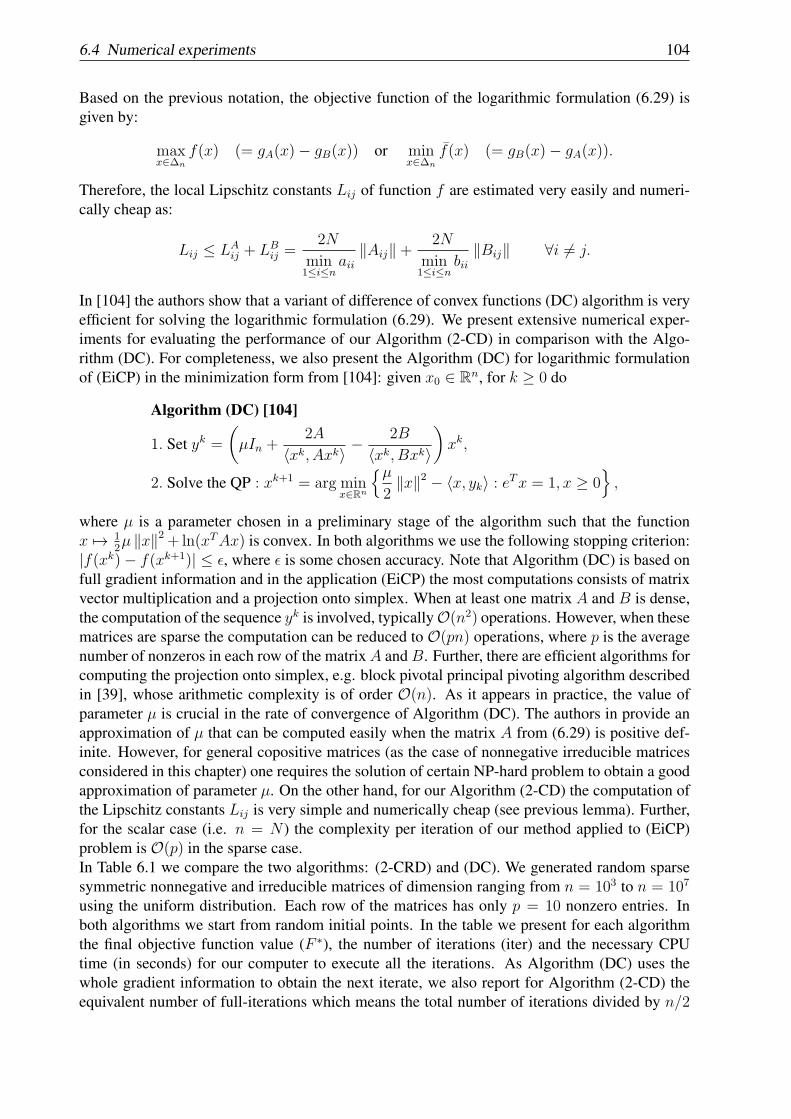
6.4 Numerical experiments 104
Based on the previous notation, the objective function of the logarithmic formulation (6.29) isgiven by:
maxx∈∆n
f(x) (= gA(x)− gB(x)) or minx∈∆n
f(x) (= gB(x)− gA(x)).
Therefore, the local Lipschitz constants Lij of function f are estimated very easily and numeri-cally cheap as:
Lij ≤ LAij + LB
ij =2N
min1≤i≤n
aii∥Aij∥+
2N
min1≤i≤n
bii∥Bij∥ ∀i = j.
In [104] the authors show that a variant of difference of convex functions (DC) algorithm is veryefficient for solving the logarithmic formulation (6.29). We present extensive numerical exper-iments for evaluating the performance of our Algorithm (2-CD) in comparison with the Algo-rithm (DC). For completeness, we also present the Algorithm (DC) for logarithmic formulationof (EiCP) in the minimization form from [104]: given x0 ∈ Rn, for k ≥ 0 do
Algorithm (DC) [104]
1. Set yk =(µIn +
2A
⟨xk, Axk⟩− 2B
⟨xk, Bxk⟩
)xk,
2. Solve the QP : xk+1 = arg minx∈Rn
µ2∥x∥2 − ⟨x, yk⟩ : eTx = 1, x ≥ 0
,
where µ is a parameter chosen in a preliminary stage of the algorithm such that the functionx 7→ 1
2µ ∥x∥2+ ln(xTAx) is convex. In both algorithms we use the following stopping criterion:
|f(xk)− f(xk+1)| ≤ ϵ, where ϵ is some chosen accuracy. Note that Algorithm (DC) is based onfull gradient information and in the application (EiCP) the most computations consists of matrixvector multiplication and a projection onto simplex. When at least one matrix A and B is dense,the computation of the sequence yk is involved, typicallyO(n2) operations. However, when thesematrices are sparse the computation can be reduced to O(pn) operations, where p is the averagenumber of nonzeros in each row of the matrixA andB. Further, there are efficient algorithms forcomputing the projection onto simplex, e.g. block pivotal principal pivoting algorithm describedin [39], whose arithmetic complexity is of order O(n). As it appears in practice, the value ofparameter µ is crucial in the rate of convergence of Algorithm (DC). The authors in provide anapproximation of µ that can be computed easily when the matrix A from (6.29) is positive def-inite. However, for general copositive matrices (as the case of nonnegative irreducible matricesconsidered in this chapter) one requires the solution of certain NP-hard problem to obtain a goodapproximation of parameter µ. On the other hand, for our Algorithm (2-CD) the computation ofthe Lipschitz constants Lij is very simple and numerically cheap (see previous lemma). Further,for the scalar case (i.e. n = N ) the complexity per iteration of our method applied to (EiCP)problem is O(p) in the sparse case.In Table 6.1 we compare the two algorithms: (2-CRD) and (DC). We generated random sparsesymmetric nonnegative and irreducible matrices of dimension ranging from n = 103 to n = 107
using the uniform distribution. Each row of the matrices has only p = 10 nonzero entries. Inboth algorithms we start from random initial points. In the table we present for each algorithmthe final objective function value (F ∗), the number of iterations (iter) and the necessary CPUtime (in seconds) for our computer to execute all the iterations. As Algorithm (DC) uses thewhole gradient information to obtain the next iterate, we also report for Algorithm (2-CD) theequivalent number of full-iterations which means the total number of iterations divided by n/2
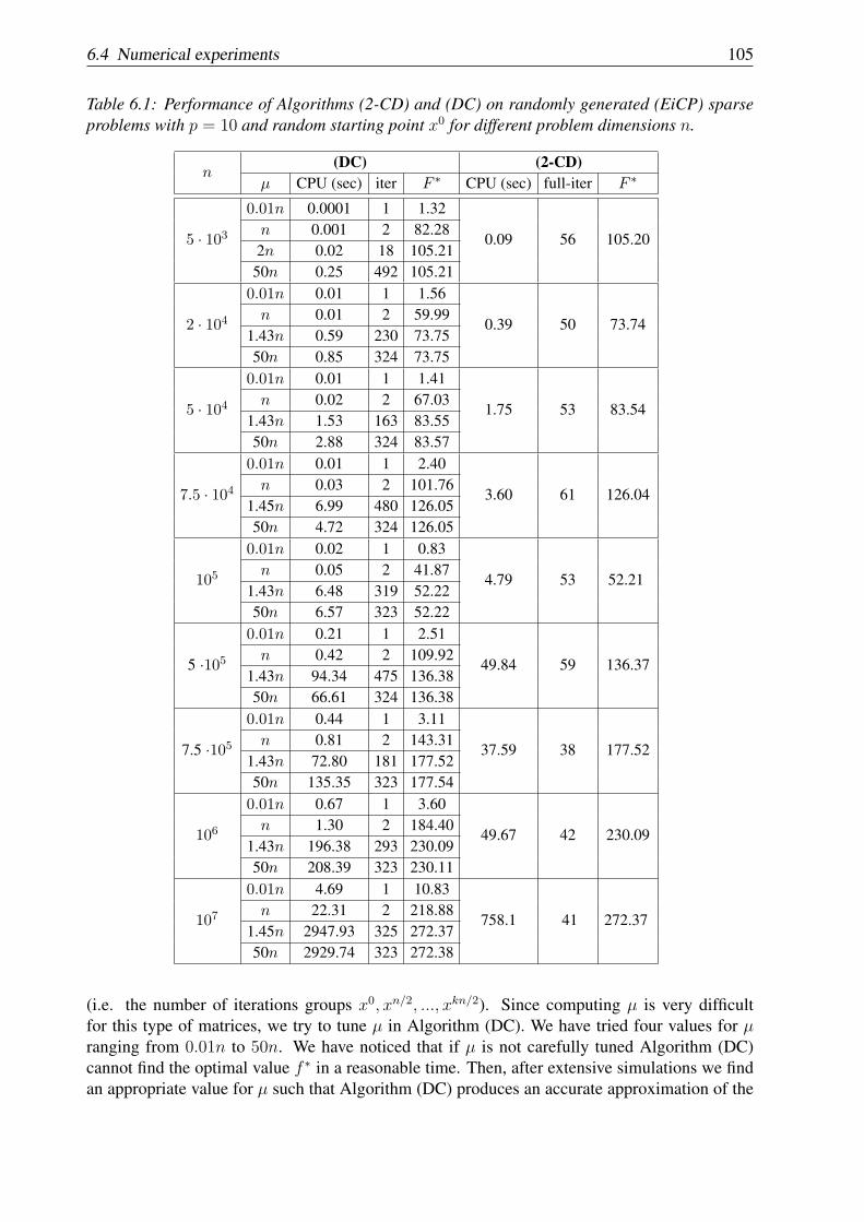
6.4 Numerical experiments 105
Table 6.1: Performance of Algorithms (2-CD) and (DC) on randomly generated (EiCP) sparseproblems with p = 10 and random starting point x0 for different problem dimensions n.
n(DC) (2-CD)
µ CPU (sec) iter F ∗ CPU (sec) full-iter F ∗
5 · 1030.01n 0.0001 1 1.32
0.09 56 105.20n 0.001 2 82.28
2n 0.02 18 105.2150n 0.25 492 105.21
2 · 1040.01n 0.01 1 1.56
0.39 50 73.74n 0.01 2 59.99
1.43n 0.59 230 73.7550n 0.85 324 73.75
5 · 1040.01n 0.01 1 1.41
1.75 53 83.54n 0.02 2 67.03
1.43n 1.53 163 83.5550n 2.88 324 83.57
7.5 · 1040.01n 0.01 1 2.40
3.60 61 126.04n 0.03 2 101.76
1.45n 6.99 480 126.0550n 4.72 324 126.05
105
0.01n 0.02 1 0.83
4.79 53 52.21n 0.05 2 41.87
1.43n 6.48 319 52.2250n 6.57 323 52.22
5 ·1050.01n 0.21 1 2.51
49.84 59 136.37n 0.42 2 109.92
1.43n 94.34 475 136.3850n 66.61 324 136.38
7.5 ·1050.01n 0.44 1 3.11
37.59 38 177.52n 0.81 2 143.31
1.43n 72.80 181 177.5250n 135.35 323 177.54
106
0.01n 0.67 1 3.60
49.67 42 230.09n 1.30 2 184.40
1.43n 196.38 293 230.0950n 208.39 323 230.11
107
0.01n 4.69 1 10.83
758.1 41 272.37n 22.31 2 218.88
1.45n 2947.93 325 272.3750n 2929.74 323 272.38
(i.e. the number of iterations groups x0, xn/2, ..., xkn/2). Since computing µ is very difficultfor this type of matrices, we try to tune µ in Algorithm (DC). We have tried four values for µranging from 0.01n to 50n. We have noticed that if µ is not carefully tuned Algorithm (DC)cannot find the optimal value f ∗ in a reasonable time. Then, after extensive simulations we findan appropriate value for µ such that Algorithm (DC) produces an accurate approximation of the
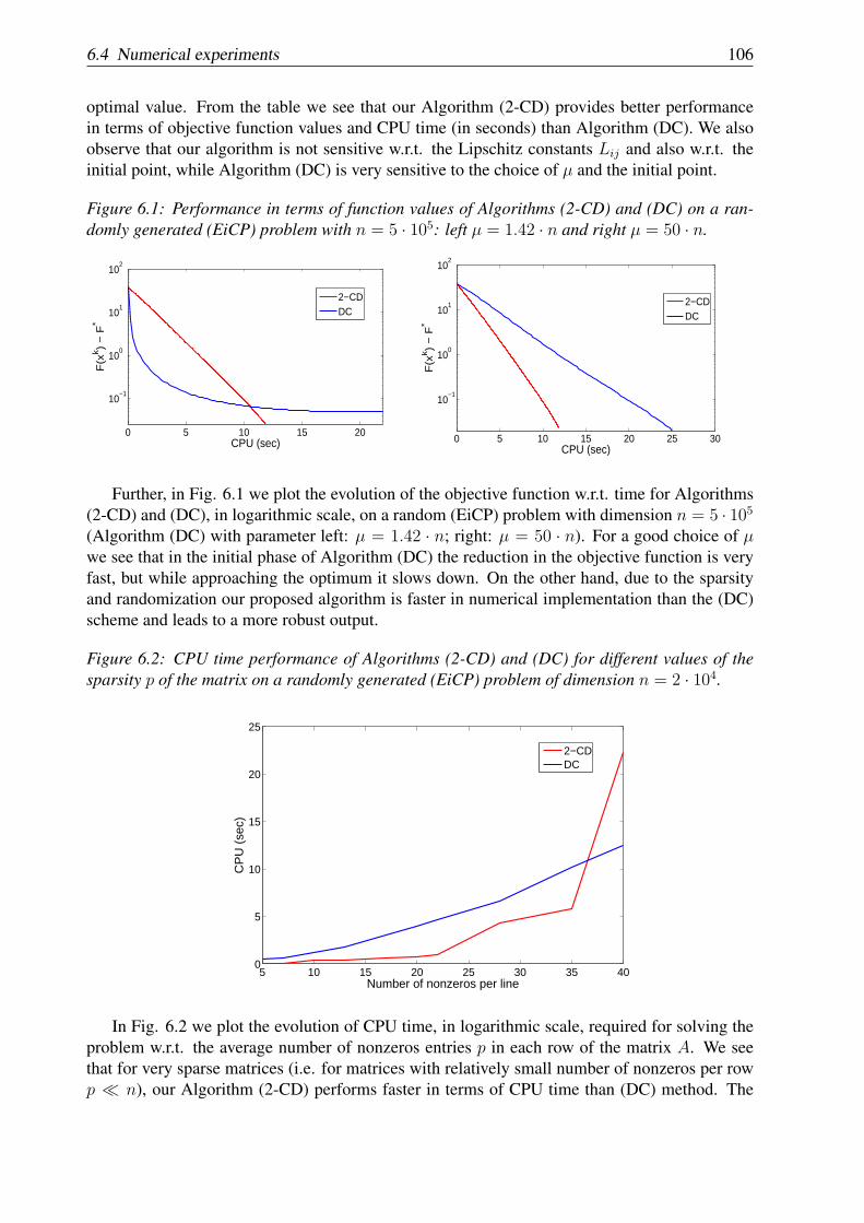
6.4 Numerical experiments 106
optimal value. From the table we see that our Algorithm (2-CD) provides better performancein terms of objective function values and CPU time (in seconds) than Algorithm (DC). We alsoobserve that our algorithm is not sensitive w.r.t. the Lipschitz constants Lij and also w.r.t. theinitial point, while Algorithm (DC) is very sensitive to the choice of µ and the initial point.
Figure 6.1: Performance in terms of function values of Algorithms (2-CD) and (DC) on a ran-domly generated (EiCP) problem with n = 5 · 105: left µ = 1.42 · n and right µ = 50 · n.
0 5 10 15 20
10−1
100
101
102
CPU (sec)
F(x
k ) −
F*
2−CDDC
0 5 10 15 20 25 30
10−1
100
101
102
CPU (sec)
F(x
k ) −
F*
2−CDDC
Further, in Fig. 6.1 we plot the evolution of the objective function w.r.t. time for Algorithms(2-CD) and (DC), in logarithmic scale, on a random (EiCP) problem with dimension n = 5 · 105(Algorithm (DC) with parameter left: µ = 1.42 · n; right: µ = 50 · n). For a good choice of µwe see that in the initial phase of Algorithm (DC) the reduction in the objective function is veryfast, but while approaching the optimum it slows down. On the other hand, due to the sparsityand randomization our proposed algorithm is faster in numerical implementation than the (DC)scheme and leads to a more robust output.
Figure 6.2: CPU time performance of Algorithms (2-CD) and (DC) for different values of thesparsity p of the matrix on a randomly generated (EiCP) problem of dimension n = 2 · 104.
5 10 15 20 25 30 35 400
5
10
15
20
25
Number of nonzeros per line
CP
U (
sec)
2−CDDC
In Fig. 6.2 we plot the evolution of CPU time, in logarithmic scale, required for solving theproblem w.r.t. the average number of nonzeros entries p in each row of the matrix A. We seethat for very sparse matrices (i.e. for matrices with relatively small number of nonzeros per rowp ≪ n), our Algorithm (2-CD) performs faster in terms of CPU time than (DC) method. The
6.4 Numerical experiments 107
main reason is that our method has a simple implementation, does not require the use of otheralgorithms at each iteration and the arithmetic complexity of an iteration is of order O(p). Onthe other hand, Algorithm (DC) is using the block pivotal principal pivoting algorithm describedin [39] at each iteration for projection on simplex and the arithmetic complexity of an iteration isof order O(pn).We conclude from the theoretical rate of convergence and the previous numerical results thatAlgorithms (1-CD) and (2-CD) are easier to be implemented and analyzed due to the random-ization and the typically very simple iteration. Furthermore, on certain classes of problems withsparsity structure, that appear frequently in many large-scale real applications, the practical com-plexity of our methods is better than that of some well-known methods from the literature. Allthese arguments make our algorithms to be competitive in the large-scale nonconvex optimizationframework. Moreover, our methods are suited for recently developed computational architectures(e.g., distributed or parallel architectures [61, 94]).

Chapter 7
Distributed random coordinate descentmethods for composite optimization
In this paper we propose a distributed version of a randomized block-coordinate descent methodfor minimizing the sum of a partially separable smooth convex function and a fully separablenon-smooth convex function. Under the assumption of block Lipschitz continuity of the gradientof the smooth function, this method is shown to have a sublinear convergence rate. Linearconvergence rate of the method is obtained for the newly introduced class of generalized errorbound functions. We prove that the new class of generalized error bound functions encompassesboth global/local error bound functions and smooth strongly convex functions. We also showthat the theoretical estimates on the convergence rate depend on the number of blocks chosenrandomly and a natural measure of separability of the objective function. Extensive numericalsimulations are also provided to confirm our theory. This chapter is based on paper [60].
7.1 IntroductionIn recent years there has been an ever-increasing interest in the optimization community for algo-rithms suitable for solving convex optimization problems with a very large number of variables.These optimization problems, known as big data problems, have arisen from more recent fieldssuch as network control [65, 72], machine learning [10] and data mining [119]. An importantproperty of these optimization problems is that they are partially separable, which permits dis-tributed and parallel computations in the optimization algorithms that are to be designed for them.This, together with the surge of multi-core machines or clustered parallel computing technologyin the past decade has led to the widespread focus on coordinate descent methods.In [77], Nesterov presents a random coordinate descent method for smooth convex problemsof large dimensions, in which only one coordinate is updated at each iteration. Under someassumption of Lipschitz gradient and strong convexity of the objective function, the algorithmin [77] was proved to have linear convergence in the expected values of the objective function.In [59,68] a 2-block random coordinate descent method is proposed to solve linearly constrainedsmooth large convex problems. The algorithm from [59,68] was extended to linearly constrainedcomposite convex minimization in [70]. The results in [77] and [79] were combined in [93], inwhich the authors propose a randomized block-coordinate descent method to solve convex prob-lems with structured composite objective functions. To our knowledge, the first results on thelinear convergence of coordinate descent methods under more relaxed assumptions than smooth-ness and strong convexity were obtained in [51, 108]. In particular, linear convergence of these
108
7.2 Problem formulation 109
methods is proved under some local error bound property, which is more general than the as-sumption of Lipschitz gradient and strong convexity as required in [59, 68, 70, 77, 93]. However,the authors in [51, 108] were able to show linear convergence only locally. Finally, very fewresults were known in the literature on distributed and parallel implementations of coordinatedescent methods. Recently, a more thorough investigation regarding the separability of the ob-jective function and ways in which the convergence can be accelerated through parallelizationwas undertaken in [68,94], where it is shown that speedup can be achieved through this approach.All of the limitations stated above motivate the work of this paper.Despite widespread use of coordinate descent methods for solving large convex problems, thereare some aspects that have not been fully studied. In particular, in practical applications, theassumption of Lipschitz gradient and strong convexity is very restrictive and the main interest isin finding larger classes of functions for which we can still prove linear convergence. We are alsointerested in providing distributed schemes, i.e. methods based on distributed and parallel com-putations. Finally, the convergence analysis has been almost exclusively limited to centralizedstepsize rules and local results. These represent the main issues that we pursue here.In this chapter we propose a distributed and parallel random (block) coordinate descent algorithmfor solving large problems with a convex separable composite objective function, i.e. consistingof the sum of a partially separable smooth function and fully separable non-smooth function.We provide a complete rate analysis of the algorithm under different assumptions and we provesubstantial improvement on the convergence rate w.r.t. the existing results from the literature. Inparticular, under the Lipschitz continuity assumption of the gradient of the smooth component,we prove sublinear rate of convergence for our distributed random coordinate descent algorithm.Further, we show that our distributed algorithm attains linear convergence for objective functionsbelonging to a general class of functions, named generalized error bound functions. We establishthat our class of functions includes the class of global/local error bound functions and implicitlystrongly convex functions with some Lipschitz continuity property on the gradient. We alsoshow that the new class of objective functions that we define in this paper covers many practicalapplications. Further, we perform a theoretical identification of which categories of problemsand objective functions satisfy the generalized error bound property. Finally, we establish that thetheoretical estimates on the convergence rate depend on the number of blocks chosen randomlyand a natural measure of separability of the objective function which is more general than theone defined in [94].In Section 7.2 we present our optimization model and discuss practical applications which canbe posed in this framework. In Section 7.3 we introduce a distributed random coordinate descentalgorithm. We prove sublinear convergence rate for this algorithm in Section 7.4. In Section7.5 we introduce the class of generalized error bound functions and we prove that our algorithmhas linear convergence rate under this property. In Section 7.6 we investigate which classesof optimization problems have an objective function that satisfies the generalized error boundproperty. Finally, in Section 7.7 we discuss distributed implementations of the algorithm andcompare it with other existing methods.
7.2 Problem formulationIn many applications arising from networks, control and data ranking, we have a system formedfrom several entities, with a communication graph which indicates the interconnections betweenentities (e.g. sources and links in network optimization [82], website pages in data ranking [10]or subsystems in control [65]). We denote this bipartite graph as G = ([N ] × [N ], E), where
7.2 Problem formulation 110
[N ] = 1, . . . , N, [N ] =1, . . . , N
and E ∈ 0, 1N×N is an incidence matrix. We also
introduce two set of neighbors Nj and Ni associated to the graph, defined as:
Nj = i ∈ [N ] : Eij = 1 ∀j ∈ [N ] and Ni = j ∈ [N ] : Eij = 1 ∀i ∈ [N ].
The index sets Nj and Ni, which e.g. in the context of network optimization may represent theset of sources which share the link j ∈ [N ] and the set of links which are used by the sourcei ∈ [N ] respectively, describe the local information flow in the graph. We denote the entirevector of variables for the graph as x ∈ Rn. The vector x can be partitioned accordingly in blockcomponents xi ∈ Rni , with n =
∑Ni=1 ni. In order to easily extract subcomponents from the
vector x, we consider a partition of the identity matrix In = [U1 . . . UN ], with Ui ∈ Rn×ni , suchthat xi = UT
i x and matrices UNi∈ Rn×nNi , such that xNi
= UTNix, with xNi
being the vectorcontaining all the components xj with j ∈ Ni. In this paper we address problems arising fromsuch systems, where the objective function can be written in a general form as (see also [81,94]):
F ∗ = minx∈Rn
F (x)
(=
N∑j=1
fj(xNj) +
N∑i=1
Ψi(xi)
), (7.1)
where fj : RnNj → R and ψi : Rni → R. We denote f(x) =∑N
j=1 fj(xNj) and Ψ(x) =∑N
i=1Ψi(xi). The function f(x) is a smooth partially separable convex function, while Ψ(x)is fully separable convex non-smooth function. The local information structure imposed by thegraph G should be considered as part of the problem formulation. We introduce the followingnatural measure of separability of the objective function F :
(ω, ω) = (maxj∈[N ]|Nj|, max
i∈[N ]|Ni|).
Note that 1 ≤ ω ≤ N , 1 ≤ ω ≤ N and our definition of the measure of separability is more gen-eral than the one introduced in [94]. It is important to note that coordinate gradient descent typemethods for solving problem (7.1) are appropriate only in the case when ω is relatively small, oth-erwise incremental type methods should be considered for solving (7.1) [114]. Indeed, difficul-ties may arise when f is the sum of a large number of component functions and ω is large, sincein that case exact computation of the components of gradient (i.e. ∇if(x) =
∑j∈Ni∇ifj(xNj
))can be either very expensive or impossible due to noise. In conclusion, we implicitly assume thatω is relatively small (i.e. ω ≪ ω ≪ n) for optimization problem (7.1).Throughout this paper, by x∗ we denote an optimal solution of problem (7.1) and by X∗ the setof optimal solutions. We define the index indicator function as:
1Nj(i) =
1, if i ∈ Nj
0, otherwise,
and the set indicator function as:
IX(x) =
0, if x ∈ X+∞, otherwise.
Also, by ∥ · ∥ we denote the standard Euclidean norm and we introduce an additional norm∥x∥2W = xTWx, where W ∈ Rn×n is a diagonal matrix with its diagonal elements Wii > 0.
7.2 Problem formulation 111
Considering these, we denote by ΠWX (x) the projection of a point x onto a set X in the norm
∥ · ∥W , i.e.:ΠW
X (x) = argminy∈X∥y − x∥2W .
Furthermore, for simplicity of exposition, we denote by x the projection of a point x on theoptimal set X∗, i.e. x = ΠW
X∗(x). In this paper we consider that the smooth component f(x) of(7.1) satisfies the following assumption:
Assumption 7.2.1 We assume that the functions fj(xNj) have Lipschitz continuous gradient with
a constant LNj> 0:
∥∇fj(xNj)−∇fj(yNj
)∥ ≤ LNj∥xNj
− yNjj∥ ∀xNj, yNj
∈ RnNj . (7.2)
Note that our assumption is different than the one in [59, 68, 77, 94], where the authors considerthat the gradient of the function f is coordinate-wise Lipschitz continuous. That is, if we definethe partial gradient ∇if(x) = UT
i ∇f(x), then there exists some constants Li > 0 such that:
∥∇if(x+ Uiyi)−∇if(x)∥ ≤ Li∥yi∥ ∀x ∈ Rn, yi ∈ Rni . (7.3)
As a consequence of Assumption 7.2.1 we have that [75]:
fj(xNj+ yNj
) ≤ fj(xNj) + ⟨∇fj(xNj
), yNj⟩+
LNj
2∥yNj∥2. (7.4)
Based on Assumption 7.2.1 we can show the following distributed variant of the descent lemma,which is central in our derivation of a distributed coordinate descent method and in proving theconvergence rate for it.
Lemma 7.2.2 Under Assumption 7.2.1 the following inequality holds for the objective functionf(x) =
∑Nj=1 fj(xNj
):
f(x+ y) ≤ f(x) + ⟨∇f(x), y⟩+ 1
2∥y∥2W ∀x, y ∈ Rn, (7.5)
where the positive definite diagonal matrix W = diag
( ∑j∈Ni
LNjIni
; i ∈ [N ]
).
Proof : If we sum up (7.4) for j ∈ [N ] and by the definition of f we have that:
f(x+ y) ≤ f(x) +N∑j=1
[⟨∇fj(xNj
), yNj⟩+
LNj
2∥yNj∥2]. (7.6)
Given matrices UNj, note that we can express the first term in the right hand side as follows:
N∑j=1
⟨∇fj(xNj
), yNj
⟩=
N∑j=1
⟨∇fj(xNj
), UTNjy⟩=
N∑j=1
⟨UNj∇fj(xNj
), y⟩=⟨∇f(x), y⟩.
Note that since W is a diagonal matrix we can express the norm ∥ · ∥W as:
∥y∥2W =N∑i=1
∑j∈Ni
LNj
∥yi∥2.
7.2 Problem formulation 112
From the definition of Nj and Ni, note that 1Nj(i) is equivalent to 1Ni
(j). Thus, for the finalterm of the right hand side of (7.6) we have that:
1
2
N∑j=1
LNj∥yNj∥2 = 1
2
N∑j=1
LNj
∑i∈Nj
∥yi∥2 =1
2
N∑j=1
LNj
N∑i=1
∥yi∥21Nj(i)
=1
2
N∑i=1
∥yi∥2N∑j=1
LNj1Ni
(j) =1
2
N∑i=1
∥yi∥2∑j∈Ni
LNj=
1
2∥y∥2W ,
and the proof is complete. 2
Note that from the generalized descent lemma through the norm ∥ · ∥W , the sparsity induced bythe graph G via the sets Nj and Ni and implicitly via the measure of separability (ω, ω) willintervene in the estimates for the convergence rates of the proposed distributed algorithm. Adetailed discussion on this issue can be found in Section 7.7. The following lemma establishesLipschitz continuity for ∇f but in the norm ∥ · ∥W , whose proof can be derived using similararguments as in [75]:
Lemma 7.2.3 For a function f satisfying Assumption 7.2.1 the following inequality holds:
∥∇f(x)−∇f(y)∥W−1 ≤ ∥x− y∥W ∀x, y ∈ Rn. (7.7)
Proof : Consider a fixed point x ∈ RN and the following optimization problem
miny∈Rn
ϕ(y) (= f(y)− ⟨∇f(x), y⟩), (7.8)
whose optimal solution is y∗ = x. By a change of variables, note that inequality (7.5) can beexpressed as:
f(x) ≤ f(y) + ⟨∇f(y), x− y⟩+ 1
2∥x− y∥2W ∀x, y ∈ RN .
By subtracting ⟨∇f(x), x − y⟩ in both sides of this inequality and by the definition of ϕ(y) in(7.8) we obtain:
ϕ(x) ≤ ϕ(y) + ⟨∇ϕ(y), x− y⟩+ 1
2∥x− y∥2W ∀x, y ∈ RN , (7.9)
i.e. ϕ(y) satisfies (7.5). Now, given that y∗ is optimal for (7.8), we have the following inequality:
ϕ(y∗) ≤ ϕ(y −W−1∇ϕ(y)
) (7.9)≤ ϕ(y)− 1
2∥∇ϕ(y)∥2W−1 .
Since∇ϕ(y) = ∇f(y)−∇f(x), then this inequality is equivalent to:
f(x) + ⟨∇f(x), y − x⟩+ 1
2∥∇f(x)−∇f(y)∥2W−1 ≤ f(y) ∀x, y ∈ Rn.
By adding two copies of the previous inequality with x and y interchanged we obtain the follow-ing:
∥∇f(x)−∇f(y)∥2W−1 ≤ ⟨∇f(x)−∇f(y), x− y⟩ ∀x, y ∈ Rn.
If we apply the Cauchy-Schwartz inequality to the right hand side of this inequality and thendivide both sides by ∥∇f(x)−∇f(y)∥W−1 , we arrive at (7.7). 2
7.2 Problem formulation 113
7.2.1 Motivating practical applicationsWe now present important applications from which the interest for problems of type (7.1) stems.Application I: One specific example is the sparse logistic regression problem. This type of prob-lem is often found in data mining or machine learning, see e.g. [43, 99, 123]. In a training setaj, bj, with j ∈ [N ], the vectors aj ∈ Rn represent N samples, and bj represent the binaryclass labels with bj ∈ −1,+1. The likelihood function for these N samples is:
N∑j=1
P(bj|aj),
where P(b|a) is the conditional probability and is expressed as:
P(b|a) = 1
1 + exp(−b⟨a, x⟩),
with x ∈ Rn being the weight vector. In some applications (see e.g. [123]), we require a bias termc (also called as an intercept) in the loss function; therefore, ⟨a, x⟩ is replaced with ⟨a, x⟩ + c.The equality ⟨a, x⟩ = 0 defines a hyperplane in the feature space on which P(b|a) = 0.5. Also,P(b|a) > 0.5 if ⟨a, x⟩ > 0 and P(b|a) < 0.5 otherwise. Then, the sparse logistic regression canbe formulated as the following convex optimization problem:
minx∈Rn
f(x) + λ ∥x∥1 ,
where λ > 0 is some constant, ∥ · ∥1 denotes the 1-norm and f(x) is the average logistic lossfunction:
f(x) = − 1
N
N∑i=1
log(P(bj|aj)
)= − 1
N
N∑j=1
log(1 + exp
(−bj⟨aj, x⟩
)).
Note that Ψ(x) = λ∥x∥1 is the separable non-smooth component which promotes the sparsity ofthe decision variable x. If we associate to this problem a bipartite graph G where the incidencematrix E is defined such that Eij = 1 provided that aji = 0, then the vectors aj have a certainsparsity according to this graph, i.e. they only have nonzero components in ajNj
. Therefore, f(x)
can be written as f(x) =∑N
j=1 fj(xNj), where each function fj is defined as:
fj(xNj) = − 1
Nlog(1 + exp
(−bj⟨ajNj
, xNj⟩))
.
It can be easily proven that the objective function f in this case satisfies (7.2) withLNj
=∑
l∈Nj∥ajl ∥2/4 and (7.3) with Li =
∑j∈Ni∥aji∥2/4. Furthermore, for this ap-
plication we have that f satisfies (7.5) with the matrix W defined as follows: W =
diag(∑
j∈Ni∥ajNj∥2/4; i ∈ [n]
).
Application II: Another classical problem which implies functions fj with Lipschitz continuousgradient of type (7.2) is:
minxi∈Xi⊆Rni
F (x)
(=
1
2∥Ax− b∥2 +
N∑i=1
λi∥xi∥1
), (7.10)
7.2 Problem formulation 114
where A ∈ RN×n, the sets Xi are convex, n =∑N
i=1 ni and λ > 0. This problem is also knownas the constrained lasso problem [36] and is widely used e.g. in signal processing, fused or gen-eralized lasso and monotone curve estimation [20, 36, 105]. For example, in image restoration,incorporating a priori information (such as box constraints on x) can lead to substantial improve-ments in the image restoration and reconstruction (see [20] for more details). Note that thisproblem is a special case of problem (7.1), with Ψ(x) =
∑Ni=1[λi∥xi∥1 + IXi
(xi)] being blockseparable and the functions fj are defined as:
fj(xNj) =
1
2(aTNj
xNj− bj)2,
where aNjare the nonzero components of row j ofA, corresponding toNj . In this application the
functions fj satisfy (7.2) with Lipschitz constants LNj= ∥aNj
∥2. Given these constants, we find
that f in this case satisfies (7.5) with W = diag(∑
j∈Ni∥aNj∥2Ini
; i ∈ [N ])
. Also, note that
functions of type (7.10) satisfy Lipschitz continuity (7.3) with Li = ∥Ai∥2, where Ai ∈ RN×ni
denotes block column i of the matrix A.Application III: A third type of problem which falls under the same category is derived from thefollowing primal formulation:
f ∗ = minu∈Rm
N∑j=1
gj(uj), (7.11)
s.t: Au ≤ b,
where A ∈ Rn×m, uj ∈ Rmj and the functions gj are strongly convex with convexity param-eters σj . This type of problem is often found in distributed control [65] or in network utilitymaximization [82]. We formulate the dual problem of (7.11) as:
maxx∈Rn
[minu∈Rm
N∑j=1
gj(uj) + ⟨x,Au− b⟩
]−Ψ(x),
where x denotes the Lagrange multiplier and Ψ(x) = IRn+(x) is the indicator function for the
nonnegative orthant Rn+. Denoting by g∗j (z) the convex conjugate of the function gj(uj), the
previous problem can be rewritten as:
f ∗ =maxx∈Rn
[N∑j=1
minuj∈Rmj
gj(uj)−⟨−AT
j x, uj⟩]− ⟨x, b⟩ −Ψ(x)
=maxx∈Rn
N∑j=1
−g∗j (−ATj x)− ⟨x, b⟩ −Ψ(x), (7.12)
where Aj ∈ Rn×mj is the jth block column of A. Note that, given the strong convexity ofgj(uj), then g∗j (z) have Lipschitz continuous gradient in z of type (7.2) with constants 1
σj[75].
Now, if the matrix A has some sparsity induced by a graph, i.e. the blocks Aij = 0 if thecorresponding incidence matrix has Eij = 0, which in turn implies that the block columns Aj
are sparse according to some index set Nj , then the matrix-vector products ATj x depend only on
xNj, such that fj(xNj
) = −g∗j(−AT
NjxNj
)− ⟨xNj
, bNj⟩, with
∑j⟨xNj
, bNj⟩ = ⟨x, b⟩. Then,
7.3 Distributed and parallel coordinate descent method 115
fj has Lipschitz continuous gradient of type (7.2) with LNj=
∥ANj∥2
σj. For this problem we
also have componentwise Lipschitz continuous gradient of type (7.3) with Li =∑
j∈Ni
∥Aij∥2σj
.
Furthermore, we find that in this case f satisfies (7.5) with W = diag(∑
j∈Ni
∥ANj∥2
σj; i ∈ [n]
).
7.3 Distributed and parallel coordinate descent methodIn this section we present in detail our distributed and parallel random coordinate descent method.Before we introduce the method however, we first need to introduce some concepts. For a func-tion F (x) as defined in (7.1), we introduce the following mapping in the norm ∥ · ∥W :
t[N ](x, y) = f(x) + ⟨∇f(x), y − x⟩+ 1
2∥y − x∥2W +Ψ(y). (7.13)
Note that the mapping t[N ](x, y) is a fully separable and strongly convex in y w.r.t. to the norm∥ · ∥W with the constant 1. We denote by T[N ](x) the proximal step for function F (x), which isthe optimal point of the mapping t[N ](x, y), i.e.:
T[N ](x) = arg miny∈Rn
t[N ](x, y). (7.14)
The step T[N ](x) can also be defined in another ways. We define the proximal operator of functionΨ as:
proxΨ(x) = arg minu∈Rn
Ψ(u) +1
2∥u− x∥2W .
We recall an important property of the proximal operator: [96]:
∥proxΨ(x)− proxΨ(y)∥W ≤ ∥x− y∥W . (7.15)
Based on this proximal operator, note that we can write:
T[N ](x) = proxΨ(x−W−1∇f(x)). (7.16)
Given that Ψ(x) is generally not differentiable, we denote by ∂Ψ(x) a vector belonging to the setof subgradients of Ψ(x). Evidently, in both definitions, the optimality conditions of the resultingproblem from which we obtain T[N ](x) are:
0 ∈∇f(x)+W (T[N ](x)−x)+∂Ψ(T[N ](x)). (7.17)
It will become evident further on that the optimal solution T[N ](x) will play a crucial role in ourrandom distributed coordinate descent method. We now establish some properties which involvethe function F (x), the mapping t[N ](x, y) and the proximal step T[N ](x). Given that t[N ](x, y) isstrongly convex in y, we have the following inequality:
F (x)− t[N ](x, T[N ](x)) = t[N ](x, x)− t[N ](x, T[N ](x))(7.17)≥ 1
2∥x− T[N ](x)∥2W . (7.18)
Further, given that f is convex and differentiable and by definition of t[N ](x, y) we get:
t[N ](x, T[N ](x)) ≤ miny∈Rn
f(y) + Ψ(y) +1
2∥y − x∥2W
= miny∈Rn
F (y) +1
2∥y − x∥2W . (7.19)
7.3 Distributed and parallel coordinate descent method 116
In the random coordinate descent algorithm that we propose we consider that at a step k ≥ 0, thecomponents of the iterate xk which are to be updated are dictated by a set of indices Jk ⊆ [N ]which is randomly chosen. Before we introduce ways in which Jk can be chosen, we needto define a number of concepts. We denote by xJ ∈ Rn the vector whose blocks xi, withi ∈ J ⊆ [N ], are identical to those of x, while the remaining blocks are zeroed out, i.e.:
xJ =
xi, i ∈ J0, otherwise.
(7.20)
Also, for the separable function Ψ(x), we denote the partial sum ΨJ(x) =∑
i∈J Ψi(xi) andthe vector ∂JΨ(x) = [∂Ψ(x)]J ∈ Rn. A random variable J is uniquely characterized by theprobability density function:
PJ = P (J = J) where J ⊆ [N ].
For the random variable J , we also define the probability with which a subcomponent i ∈ [N ]can be found in J as:
pi = P(i ∈ J).
In our algorithm, we consider a uniform sampling of τ unique coordinates i, 1 ≤ τ ≤ N thatmake up J , i.e. |J | = τ . For a random variable J with |J | = τ , we observe that we have atotal number of
(Nτ
)possible values that J can take, and with the uniform sampling we have that
PJ = 1
(Nτ ). Given that J is random, we can express the probability that i ∈ J as:
pi =∑J : i∈J
PJ .
For a single index i, note that we have a total number of(N−1τ−1
)possible sets that J can take
which will include i and therefore the probability that this index is included in J is:
pi =
(N−1τ−1
)(Nτ
) =τ
N. (7.21)
Remark 7.3.1 We can also consider other ways in which J can be chosen. For example, we canhave partition sets J1, . . . , Jq of [N ], i.e. [N ] =
∪qi=1 J
i, that are randomly shuffled. We can alsochoose J in a nearly independent manner, i.e. J is chosen with a sufficient probability, or we canchoose J according to an irreducible and aperiodic Markov chain, see e.g. [108, 114]. However,if we employ these strategies for choosing J , the proofs for the convergence rate of our algorithmfollow similar lines. 2
Having defined the proximal step as T[N ](xk) in (7.14), in the algorithm that follows we generate
randomly at step k an index set Jk of cardinality 1 ≤ τ ≤ N . We denote the vector TJk(xk) =[T[N ](x
k)]Jk which will be used to update xk+1, i.e. in the sense that [xk+1]Jk = TJk(xk). Also,by Jk we denote the complement set of Jk, i.e. Jk = i ∈ [N ] : i /∈ Jk. Thus, our methodconsists of the following steps:

7.3 Distributed and parallel coordinate descent method 117
Distributed and parallel random coordinate descent method (D-RCD)
1. Consider an initial point x0 ∈ Rn
2. For k ≥ 0:
2.1 Generate with uniform probability a random set of indices Jk ⊆ [N ],with |Jk| = τ
2.2 Compute:
xk+1Jk = TJk(xk) and xk+1
Jk = xkJk .
Note that the iterate update of (D-RCD) method can be expressed in the following ways:xk+1 = xk + TJk(xk)− xkJk
xk+1 = argminy∈Rn⟨∇Jkf(xk), y − xk⟩+ 12∥y − xk∥2W +ΨJk(y)
xk+1 = proxΨJk
(xk −W−1∇Jkf(xk)
).
(7.22)
Note that the right hand sides of the last two equalities contain the same optimization problemwhose optimality conditions are:
W [xk − xk+1]Jk ∈ ∇Jkf(xk) + ∂ΨJk(xk+1)
[xk+1]Jk = [xk]Jk .(7.23)
Clearly, the optimization problem from which we compute the iterate of (D-RCD) is fully sep-arable. Then, it follows that for updating component i ∈ Jk of xk+1 we need the followingdata: Ψi(x
ki ),Wii and∇if(x
k). However, the ith diagonal entry Wii =∑
j∈NiLNj
and ith blockcomponent of the gradient ∇if =
∑j∈Ni∇ifj can be computed distributively according to the
communication graph G imposed on the original optimization problem. Therefore, if algorithm(D-RCD) runs on multi-core machine or as a multi-thread process, it can be observed that com-ponent updates can be done distributively and in parallel by each core/thread (see Section 7.7 formore details).We now establish that method (D-RCD) is a descent method, i.e. F (xk) ≤ F (x0) for all k ≥ 0.From the convexity of Ψ(·) and (7.5) we obtain the following:
F (xk+1) ≤ F (xk)+⟨∇f(xk), xk+1−xk⟩+⟨∂Ψ(xk+1), xk+1−xk⟩+1
2∥xk+1−xk∥2W
= F (xk) + ⟨∇Jkf(xk) + ∂ΨJk(xk), [xk+1 − xk]Jk⟩+ 1
2∥xk+1 − xk∥2W
(7.23)= F (xk) + ⟨W [xk − xk+1]Jk , [xk+1 − xk]Jk⟩+ 1
2∥xk+1 − xk∥2W
= F (xk)− 1
2∥xk+1 − xk∥2W . (7.24)
With (D-RCD) being a descent method, we can now introduce the following term:
RW (x0) = maxx: F (x)≤F (x0)
maxx∗∈X∗
∥x− x∗∥W . (7.25)
and assume it to be bounded. We also define the random variable comprising the whole historyof previous events as:
ηk = J0, . . . , Jk.
7.4 Sublinear convergence for smooth convex minimization 118
7.4 Sublinear convergence for smooth convex minimizationIn this section we establish the sublinear convergence rate of method (D-RCD) for problems oftype (7.1) with the objective function satisfying Assumption 7.2.1.The following lemma provides some essential properties for the uniform sampling with |J | = τ ,which was also stated in Lemma 3 in [94]. For completness we also give the proof.
Lemma 7.4.1 Let there be some constants θi with i = 1, . . . , N , and a sampling J chosen asdescribed above and define a sum θJ =
∑i∈J θi. Then, the expected value of the sum θJ satisfies:
E [θJ ] =N∑i=1
piθi. (7.26)
Proof : We denote the series of the total number of sets of cardinality τ that the random variableJ can take by Jl, with l = 1, . . . ,
(Nτ
). We can express in detail the expected value E[θJ ]:
E[θJ ] =∑J⊆[N ]
(∑i∈J
θi
)PJ =
(Nτ )∑l=1
PJl
(N∑i=1
θi1Jl(i)
)=
N∑i=1
θi
(Nτ )∑l=1
PJl1Jl(i)
=N∑i=1
θi∑J :i∈J
PJ =N∑i=1
piθi
and the proof is complete 2.
For a vector d ∈ Rn, consider its counterpart dJ for a sampling J taken as described above.Given this lemma and by taking into account the separability of the inner product, of the squared∥ · ∥2W norm and of the function Ψ(x) , it follows that:
E [⟨x, dJ⟩] =τ
N⟨x, d⟩, (7.27)
E[∥dJ∥2W
]=
τ
N∥d∥2W (7.28)
E [Ψ(x+ dJ)] =τ
NΨ(x+ d) +
(1− τ
N
)Ψ(x). (7.29)
The following lemma provides an essential relation for the convergence rate analysis of (D-RCD)method.
Lemma 7.4.2 Consider functions f and Ψ defined in (7.1), with f satisfying Assumption 7.2.1,and the matrixW as defined in Lemma 7.2.2. Also, for any h, x ∈ Rn, consider a vector y = h−xand corresponding vector yJ = hJ − xJ . Then, the expected value E [f(x+ yJ)] satisfies:
E [f(x+ yJ)] ≤ f(x) +τ
N
(⟨∇f(x), y⟩+ 1
2∥y∥2W
), (7.30)
and furthermore:E[F (x+yJ)] ≤
(1− τ
N
)F (x) +
τ
Nt[N ](x, h). (7.31)

7.4 Sublinear convergence for smooth convex minimization 119
Proof : If we replace y with yJ in (7.5) and apply the expectation in J to both sides of theinequality we get:
E[f(x+ yJ)] ≤f(x)+ E[⟨∇f(x), yJ⟩+
1
2∥yJ∥2W
](7.27),(7.28)≤ f(x)+
τ
N
(⟨∇f(x), y⟩+1
2∥y∥2W
).
Regarding the second part of the lemma, note that we can express:
E[F (x+yJ)]= E [f(x+ yJ) + Ψ(x+ yJ)]
(7.29),(7.30)≤ f(x)+
τ
N
(⟨∇f(x), y⟩+ 1
2∥y∥2W
)+(1− τ
N
)Ψ(x) +
τ
NΨ(x+ y)
(7.13)=(1− τ
N
)F (x) +
τ
Nt[N ](x, h)
and the proof is complete. 2
We can now formulate an important relation between the operator t[N ](x, T[N ](x)) for a point xand the optimal value F (x∗). Consider a point y(α) which is a convex combination of x∗ and x:
y(α) = αx∗ + (1− α)x with α ∈ [0, 1].
For a point x, with F (x) ≤ F (x0), following the definition of the operator t[N ](x, y) and throughthe convexity of F we obtain the following inequality :
t[N ](x, T[N ](x))(7.19)≤ min
y∈RnF (y) +
1
2∥y − x∥2W
y=y(α)
≤ minα∈[0,1]
F (αx∗ + (1− α)x) + α2
2∥x− x∗∥2W
(7.25)≤ min
α∈[0,1]F (x)− α(F (x)− F (x∗)) + α2
2(RW (x0))2. (7.32)
Note that for the optimization problem in the last inequality the optimal solution is:
α∗ = min
1,F (x)− F (x∗)(RW (x0))2
,
and by replacing it in (7.32) we obtain:
t[N ](x,T[N ](x))− F ∗ ≤
12(RW (x0))2 < 1
2(F (x)− F ∗), if α∗ = 1(
1− F (x)−F ∗
2(RW (x0))2
)(F (x)− F ∗), if α∗ < 1.
(7.33)
This property will prove useful in the following theorem, that is the main result of this section,which provides the sublinear convergence rate for method (D-RCD).
Theorem 7.4.3 If Assumption 7.2.1 holds and RW (x0) defined in (7.25) is bounded, then aslong as F (xk) − F (x∗) > (RW (x0))2 and xk generated by (D-RCD) we have the followingconvergence rate:
E[F (xk)]− F ∗ ≤(1− τ
2N
)k(F (x0)− F ∗), (7.34)
7.4 Sublinear convergence for smooth convex minimization 120
Overall, we have that the sequence xk generated by algorithm (D-RCD) satisfies the followingglobal convergence rate for the expected values of the objective function:
E[F (xk)]− F ∗ ≤ 2N max (RW (x0))2, F (x0)− F ∗τk + 2N
∀k ≥ 0. (7.35)
Proof : By taking expectation in both sides of (7.24) w.r.t. Jk conditioned on ηk−1 we arrive at:
E[F (xk+1)] ≤ F (xk)− 1
2E[∥xk+1 − xk∥2W
]≤ F (xk). (7.36)
Now, if we take x = xk and yJk = TJk(xk)− xkJk in (7.31) we get:
E[F (xk+1)
]≤(1− τ
N
)F (xk) +
τ
Nt[N ]
(xk, T[N ](x
k)). (7.37)
Thus, given that F (xk)− F ∗ > (RW (x0))2 we have that:
E[F (xk+1)
]− F ∗ ≤
(1− τ
N
)(F (xk)− F ∗) +
τ
N
(t[N ]
(xk, T[N ](x
k))− F ∗)
(7.33)≤(1− τ
N
)(F (xk)− F ∗) +
τ
2N
(F (xk)− F ∗)
=(1− τ
2N
)(F (xk)− F ∗).
If we now take expectation over ηk−1 and we apply this inequality repeatedly we obtain (7.34).For the second part of the proof note that:
E[F (xk+1)]− F ∗ ≤(1− τ
N
)(F (xk)− F ∗) +
τ
N
(t[N ]
(xk, T[N ](x
k))− F ∗)
(7.33)≤(1− τ
N+τ
Nmax
1− F (xk)−F ∗
2(RW (x0))2,1
2
)(F (xk)−F ∗)
= max
1− τ
N
F (xk)− F ∗
2(RW (x0))2, 1− τ
2N
(F (xk)−F ∗).
Further, from (7.36) we have that E[F (xk+1)] ≤ F (xk). Thus, if we define c =2N
τmax (RW (x0))2, F (x0)− F ∗, then from the previous inequality we derive the following:
E[F (xk+1)]− F ∗ ≤(1− F (xk)− F ∗
c
)(F (xk)− F ∗) . (7.38)
If we now denote δk = F (xk) − F ∗ and take expectation over ηk−1 in the above inequality wearrive at:
E[δk]− E[δk+1] ≥ (E[δk])2
c.
Through this inequality we can derive the following:
1
E[δk+1]− 1
E[δk]=
E[δk]− E[δk+1]
E[δk]E[δk+1]≥ E[δk]− E[δk+1]
(E[δk])2≥ 1
c.
Furthermore, if we sum up these inequalities we obtain the following:
1
E[δk]≥ 1
E[δ0]+k
c.
which leads to (7.35). 2
7.5 Linear convergence for error bound convex minimization 121
We notice that given the choice of τ we get different results (see Section 7.7 for a detailedanalysis). For τ = 1 we obtain a similar convergence rate to that of the random coordinatedescent method in [79], while for τ = N we get a similar convergence rate to that of the fullcomposite gradient method of [77]. Note that our results are also similar with those of [94] butare obtained under completely different assumptions regarding the objective function and witha different analysis. We notice that the convergence rate depends on the choice of τ = |J |. Ifthe algorithm is implemented on a multi-core machine or cluster, then τ reflects the availablenumber of cores.The following corollary establishes the number of necessary iterates kϵρ which will ensure anϵ-suboptimal solution with probability at least 1− ρ:
Corollary 7.4.4 Under Assumption 7.2.1 and with RW (x0) defined in (7.25) bounded, consideran suboptimality level ϵ and a probability level ρ. Then, for the iterates generated by algorithm(D-RCD) and an kϵρ that satisfies:
kϵρ ≥ 2 +2N max (RW (x0))2, F (x0)− F ∗
τϵ
(1− ϵ
F (x0)− F ∗ + log(1/ρ)
)we have that:
P(F(xk
ϵρ)− F ∗ ≤ ϵ
)≥ 1− ρ.
Proof : Denote δk = F (xk) − F ∗ as in Theorem 7.4.3. Then, from (7.38) we have that δk
satisfies
E[δk+1|δk] ≤(1− δk
c
)δk for all k such that δk ≥ ϵ,
where 0 ≤ ϵ ≤ δ0 and c defined in Theorem 7.4.3. Since from (7.36) we have that δk+1 ≤ δk, wecan choose ϵ ≤ δ0 and can apply Lemma 3.8.1 from Chapter 3 to δk and the proof is complete.
2
7.5 Linear convergence for error bound convex minimizationIn this section we prove that, for certain minimization problems, the sublinear convergence rateof (D-RCD) from the previous section can be improved to a linear convergence rate. In particular,we prove that under additional assumptions on the objective function, which are often satisfiedin practical applications (e.g. dual of a linearly constrained smooth convex problem or controlproblem), we have a generalized error bound property for our optimization problem. In thesesettings we analyze the convergence behavior of the randomized algorithm (D-RCD) for whichwe are able to provide for the first time global linear convergence rate, as opposed to the resultsin [51,108] where only local linear convergence was derived for deterministic descent methods orthe results in [115] where global linear convergence is proved for a gradient method but appliedonly to problems where Ψ is the set indicator function of a bounded polyhedron or Rn.We introduce the proximal gradient mapping of function F (x):
∇+F (x) = x− proxΨ
(x−W−1∇f(x)
). (7.39)
Clearly, a point x∗ is an optimal solution of problem (7.1) if and only if ∇+F (x∗) = 0. In thefollowing definition we introduce the concept of Generalized Error Bounded Functions (GEBF):
7.5 Linear convergence for error bound convex minimization 122
Definition 7.5.1 A function F has the generalized error bound property w.r.t. the norm ∥ · ∥W ifit satisfies the following relation:
∥x− x∥W ≤(κ1 + κ2∥x− x∥2W
)∥∇+F (x)∥W ∀x ∈ Rn, (7.40)
where κ1 and κ2 are two nonnegative constants and x = ΠWX∗(x). 2
Remark 7.5.2 Note that the class of functions introduced in (7.40) includes other known cate-gories of functions:(i) For example, functions F composed of a strongly convex function f with a convex constantσW w.r.t. the norm ∥ · ∥W and a general convex function Ψ satisfy our definition (7.40) withκ1 =
2σW
and κ2 = 0, see Section 7.6 for more details.(ii) For the particular case where Ψ is the indicator function of a bounded polyhedron or of theentire space Rn, in [115] the authors establish conditions for which a function F has a globalerror bound property, i.e.:
∥x− x∥ ≤ κ∥∇+F (x)∥ ∀x ∈ Rn, (7.41)
where κ is a positive constant. Clearly, these functions satisfy our definition (7.40) with κ1 =
κ√
maxi Wii
mini Wiiand κ2 = 0.
(iii) In [108] the authors establish conditions for which a function F has a local error boundproperty, i.e. there exist κ and ϑ such that:
∥x− x∥ ≤ κ∥∇+F (x)∥ ∀x satisfying ∥∇+F (x)∥ ≤ ϑ. (7.42)
Clearly, for x satisfying ∥∇+F (x)∥ > ϑ there exists ϱϑ such ∥x−x∥ ≥ ϱϑ. Thus, these functions
satisfies our definition (7.40) with κ1 = κ√
maxi Wii
mini Wiiand κ2 =
√maxi Wii
mini Wii
1ϑϱϑ
. 2
Next, we prove that on optimization problems having the (GEBF) property (7.40) our algorithm(D-RCD) has global linear convergence. Our analysis will use ideas from the proof of determin-istic descent methods in [108]. However, the random nature of our method and the the nonsmoothproperty of the objective function requires a new approach. For example, the typical proof forlinear convergence of gradient descent type methods for solving convex problems with an errorbound like property is based on deriving an inequality of the form F (xk+1)−F ∗ ≤ c∥xk+1−xk∥(see e.g. [51, 108, 115]). Under our settings, we cannot derive this type of inequality but insteadwe obtain a weaker inequality that still allows us to prove linear convergence (see (7.56) below).We start with the following lemma which shows an important property of algorithm (D-RCD)when it is applied to problems having generalized error bound objective function:
Lemma 7.5.3 If a function F satisfies (GEBF) given in (7.40), then a point xk generated byalgorithm (D-RCD) and its projection onto X∗, denoted xk, satisfy the following:
∥xk − xk∥2W ≤(κ1 + κ2∥xk − xk∥2W
)2 NτE[∥xk+1 − xk∥2W
]. (7.43)
Proof : For the iteration defined by algorithm (D-RCD) we have:
E[∥xk+1 − xk∥2W
]= E
[∥xk + TJk(xk)− xkJk − xk∥2W
]= E
[∥xkJk − TJk(xk)∥2W
] (7.28)=
τ
N∥xk − T[N ](x
k)∥2W
=τ
N∥xk − proxΨ(x
k −W−1∇f(xk))∥2W
=τ
N∥∇+F (xk)∥2W .

7.5 Linear convergence for error bound convex minimization 123
Through this equality and (7.40) we have that:
∥xk − xk∥2W ≤ (κ1 + κ2∥xk − xk∥2W )2∥∇F+(xk)∥2W
≤ (κ1 + κ2∥xk − xk∥2W )2N
τE[∥xk+1 − xk∥2W
], (7.44)
and the proof is complete. 2
Remark 7.5.4 Note that if the iterates of an algorithm satisfy the following relation:
∥xk − x∗∥ ≤ ∥x0 − x∗∥ ∀k ≥ 1,
see e.g. the case of the full gradient method [75], then we have:
∥xk − xk∥2W ≤κ(x0)N
τE[∥xk+1 − xk∥2W
]∀k ≥ 0, (7.45)
where κ(x0) = (κ1 + κ2∥x0 − x∗∥2W )2.
If the iterates of an algorithm satisfy (7.25) with RW (x0) bounded, see e.g. the case of ouralgorithm (D-RCD) which is a descent method, as proven in (7.24), then (7.45) is satisfied withκ(x0) = (κ1 + κ2RW (x0)2)2. 2
Since the function Ψ(x) is fully separable, we obtain the following lemma:
Lemma 7.5.5 Given a fully separable function Ψ : Rn → R and a vector d ∈ Rn, consider theircounterparts ΨJ and dJ for a sampling J taken as described above. Then, the expected valueE [ΨJ(dJ)] satisfies:
E [ΨJ(dJ)] =τ
NΨ(d). (7.46)
Proof : From the definition of expectation and Lemma 7.4.1 we obtain the following:
E[ΨJ(dJ)] =∑J⊆[N ]
(∑i∈J
Ψi(di)
)PJ =
N∑i=1
Ψi(di)∑J :i∈J
PJ
=N∑i=1
piΨi(di)(7.21)=
τ
N
N∑i=1
Ψi(di) =τ
NΨ(d).
and the proof is complete. 2
Considering now that xk ∈ X∗, then from (7.43) we obtain:∥∥xk − xk∥∥W≤ cκ(τ)
√E [∥xk+1 − xk∥2], (7.47)
where cκ(τ) = (κ1 + κ2RW (x0)2)√
Nτ
. We now need to express E[Ψ(xk+1)] explicitly, where
xk+1 is generated by algorithm (D-RCD). Note that xk+1Jk = xk
Jk . As a result, we have:
E[Ψ(xk+1)] = E
[∑i∈Jk
Ψi
([TJk(xk)]i
)+∑i∈Jk
Ψi
([xk]i
)](7.46)=
τ
NΨ(T[N ](x
k))+N − τN
Ψ(xk). (7.48)
The following lemma establishes an important upper bound for E[F (xk+1)−F (xk)
].
7.5 Linear convergence for error bound convex minimization 124
Lemma 7.5.6 If function F satisfies Assumption 7.2.1 and the (GEBF) property defined in(7.40), then the iterate xk generated by (D-RCD) method has the following property:
E[F (xk+1)− F (xk)
]≤ E[Λk] ∀k ≥ 0, (7.49)
whereΛk = ⟨∇f(xk), xk+1 − xk⟩+ 1
2∥xk+1 − xk∥2W +Ψ(xk+1)−Ψ(xk).
Furthermore, we have that:1
2∥xk+1 − xk∥2W ≤ −Λk ∀k ≥ 0. (7.50)
Proof : Taking x = xk and y = xk+1 − xk in (7.5) we get:
f(xk+1) ≤ f(xk) + ⟨∇f(xk), xk+1 − xk⟩+ 1
2∥xk+1 − xk∥2W .
By adding Ψ(xk+1) and substracting Ψ(xk) in both sides of this inequality and by taking expec-tation in both sides we obtain (7.49). Recall the iterate update (7.22) of our algorithm (D-RCD):
xk+1 = arg miny∈Rn
⟨∇Jkf(xk), y − xk⟩+ 1
2∥y − xk∥2W +ΨJk(y).
Given that xk+1 is optimal for the problem above and if we take a vector y = αxk+1+(1−α)xk,for α ∈ [0, 1], we have that:
⟨∇Jkf(xk), xk+1 − xk⟩+ 1
2∥xk+1 − xk∥2W +ΨJk(xk+1)
≤ α⟨∇Jkf(xk), xk+1 − xk⟩+ α2
2∥xk+1 − xk∥2W +ΨJk(αxk+1 + (1− α)xk).
Further, if we rearrange the terms and through the convexity of ΨJk we obtain:
(1− α)[⟨∇Jkf(xk), xk+1−xk⟩+ 1 + α
2∥xk+1−xk∥2W +ΨJk(xk+1)−ΨJk(xk)
]≤ 0.
If we divide this inequality by (1− α) and let α ↑ 1 we have that:
⟨∇Jkf(xk), xk+1 − xk⟩+ (ΨJk(xk+1)−ΨJk(xk)) ≤ −∥xk+1 − xk∥2W .By adding 1
2∥xk+1 − xk∥2W in both sides of this inequality and observing that:
⟨∇Jkf(xk), xk+1 − xk⟩ = ⟨∇f(xk), xk+1 − xk⟩ and
ΨJk(xk+1)−ΨJk(xk) = Ψ(xk+1)−Ψ(xk),
we obtain (7.50). 2
Additionally, note that by applying expectation in Jk to Λk we get:
E[Λk](7.27),(7.28)
=τ
N⟨∇f(xk), T[N ](x
k)− xk⟩+ 1
2E[∥xk+1 − xk∥2W
]+ E
[Ψ(xk+1)
]−Ψ(xk)
(7.48)=
τ
N⟨∇f(xk), T[N ](x
k)− xk⟩+ 1
2E[∥xk+1 − xk∥2W
](7.51)
+τ
N
(Ψ(T[N ](x))−Ψ(xk)
).
The following theorem, which is the main result of this section, proves the linear convergencerate for the algorithm (D-RCD) on optimization problems having the generalized error boundproperty.
7.5 Linear convergence for error bound convex minimization 125
Theorem 7.5.7 On optimization problems (7.1) with the objective function satisfying Assump-tion 7.2.1 and the generalized error bound property (7.40), the algorithm (D-RCD) has the fol-lowing global linear convergence rate for the expected values of the objective function:
E[F (xk)− F ∗] ≤ θk(F (x0)− F ∗) ∀k ≥ 0, (7.52)
where θ < 1 is a constant depending on N, τ, κ1, κ2 and RW (x0).
Proof : We first need to establish an upper bound for E[F (xk+1)]− F (xk). By the definition ofF and its convexity we have that:
F (xk+1)− F (xk)= f(xk+1)− f(xk) + Ψ(xk+1)−Ψ(xk)
≤ ⟨∇f(xk+1), xk+1 − xk⟩+Ψ(xk+1)−Ψ(xk)
= ⟨∇f(xk+1)−∇f(xk), xk+1 − xk⟩+ ⟨∇f(xk), xk+1 − xk⟩+Ψ(xk+1)−Ψ(xk)
≤ ∥∇f(xk+1)−∇f(xk)∥W−1∥xk+1−xk∥W + ⟨∇f(xk), xk+1−xk⟩+Ψ(xk+1)−Ψ(xk)(7.7)≤ ∥xk+1−xk∥W∥xk+1 − xk∥W + ⟨∇f(xk), xk+1 − xk⟩+Ψ(xk+1)−Ψ(xk)
≤ ∥xk+1−xk∥2W+∥xk+1−xk∥W∥xk−xk∥W+⟨∇f(xk), xk+1−xk⟩+Ψ(xk+1)−Ψ(xk).
By taking expectation in both sides of the previous inequality we have:
E[F (xk+1)]− F (xk) ≤ E[∥xk+1 − xk∥2W ] + E[∥xk+1−xk∥W∥xk−xk∥W
]+ E
[⟨∇f(xk), xk+1 − xk⟩+Ψ(xk+1)
]−Ψ(xk). (7.53)
From (7.25) we have that ∥xk − xk∥ ≤ RW (x0) and derive the following:
E[∥xk+1−xk∥W∥xk−xk∥W
]= ∥xk−xk∥WE
[∥xk+1−xk∥W
](7.47)≤ cκ(τ)
√E [∥xk+1−xk∥2W ]
√(E [∥xk+1−xk∥W ])2
≤ cκ(τ) E[∥xk+1−xk∥2W
],
where the last step comes from Jensen’s inequality. Thus, (7.53) becomes:
E[F (xk+1)]− F (xk) ≤ c1(τ)E[∥xk+1−xk∥2W ]+E[⟨∇f(xk), xk+1−xk
⟩]+ E[Ψ(xk+1)]−Ψ(xk), (7.54)
where c1(τ) =(1+cκ(τ)). We now explicitly express the second term in the right hand side ofthe above inequality:
E[⟨∇f(xk), xk+1 − xk⟩
] (7.22),(7.28)=
τ
N⟨∇f(xk), T[N ](x
k)− xk⟩.
So, by replacing it in (7.54) and through (7.48) we get:
E[F (xk+1)]− F (xk) ≤ c1(τ)E[∥xk+1 − xk∥2W ] +τ
N⟨∇f(xk), T[N ](x
k)− xk⟩
+τ
NΨ(T[N ](x
k)) +N − τN
Ψ(xk)−Ψ(xk).
7.5 Linear convergence for error bound convex minimization 126
By rearranging the terms, we obtain the following:
E[F (xk+1)]− F (xk) (7.55)
≤ c1(τ)E[∥xk+1−xk∥2W ]+⟨∇f(xk) + (W −W )(T[N ](x
k)− xk), T[N ](xk)− xk
⟩+Ψ(T[N ](x
k))−Ψ(xk)+N−τN
(Ψ(xk)−Ψ(T[N ](x))−⟨∇f(xk), T[N ](x
k)− xk⟩).
Now, from the optimality conditions of (7.16) and Fermat’s rule [96] we derive the followinginequality:
⟨∇f(xk) +W (T[N ](xk)− xk), T[N ](x
k)− xk⟩+Ψ(T[N ](x))
≤ ⟨∇f(xk) +W (T[N ](xk)− xk), xk − xk⟩+Ψ(xk),
and as a result:
⟨∇f(xk) +W (T[N ](xk)− xk), T[N ](x
k)− xk⟩+Ψ(T[N ](xk))−Ψ(xk) ≤ 0.
By replacing this inequality in (7.55) we get:
E[F (xk+1)]− F (xk) ≤ c1(τ)E[∥xk+1 − xk∥2W ]−⟨W (T[N ](xk)−xk), T[N ](x
k)−xk⟩
+N − τN
(Ψ(xk)−Ψ(T[N ](x
k))− ⟨∇f(xk), T[N ](xk)− xk⟩
)= cκ(τ) E[∥xk+1 − xk∥2W ]−⟨W (T[N ](x
k)−xk), xk − xk⟩
+N − τN
(Ψ(xk)−Ψ(T[N ](x
k))− ⟨∇f(xk), T[N ](xk)− xk⟩
)(7.51)= cκ(τ) E[∥xk+1 − xk∥2W ]−⟨W (T[N ](x
k)−xk), xk − xk⟩
+N−ττ
(1
2E[∥xk+1 − xk∥2W ]− E[Λk]
)≤(cκ(τ)+
N−τ2τ
)E[∥xk+1−xk∥2W ]
+∥T[N ](xk)−xk∥W∥xk−xk∥W +
τ −Nτ
E[Λk]
(7.47)≤
(cκ(τ)
(1+
√N
τ
)+N−τ2τ
)E[∥xk+1−xk∥2W ] +
τ−Nτ
E[Λk].
From this inequality and (7.50) we get:
E[F (xk+1)]− F (xk) ≤ −c2(τ)E[Λk], (7.56)
where c2(τ) = 2(cκ(τ)(1 +
√N/τ)+ N−τ
τ
)> 0. Furthermore, from (7.49) we obtain:
E[F (xk+1)]− F (xk) ≤ c2(τ)(F (xk)− E[F (xk+1)]
),
from which by rearranging E[F (xk+1)] and substracting c2(τ)F (xk) in both sides we get:
E[F (xk+1)
]− F (xk) ≤ c2(τ)
1 + c2(τ)
(F (xk)− F (xk)
). (7.57)
We denote θ = c2(τ)1+c2(τ)
< 1 and denote δk = F (xk+1)− F (xk). By taking expectation over ηk−1
in (7.57) we arrive at:E[δk] ≤ θE[δk−1] ≤ · · · ≤ θkE[δ0],
and linear convergence is proved. 2
7.5 Linear convergence for error bound convex minimization 127
Note that we have obtained for the first time global linear convergence for our distributed ran-dom coordinate descent method on the general class of problems satisfying the generalized errorbound property (GEBF) given in (7.40), as opposed to the results in [51, 108] where the authorsonly show local linear convergence for deterministic coordinate descent methods applied to localerror bound functions, i.e. for all k ≥ k0 > 1, where k0 is an iterate after which some conditionsare implicitly satisfied (see Remark 7.5.2 (iii) and (7.42)). In [115] global linear convergenceis also proved for the full gradient method but applied only to problems having the error boundproperty where Ψ is the set indicator function of a bounded polyhedron or Rn (see Remark 7.5.2(ii) and (7.41)). Moreover, our results are more general than the ones in [59,68,77,94], where theauthors prove linear convergence for the more restricted class of problems having smooth andstrongly convex objective function and our proof for convergence is completely different fromthose in these papers.
We now establish the number of iterations kϵρ which will ensure a ϵ-suboptimal solution withprobability at least 1− ρ. In order to do so, we recall the well-known lemma:
Lemma 7.5.8 For constants ϵ > 0 and γ ∈ (0, 1) such that δ0 > ϵ > 0 and k ≥ 1γlog(
δ0
ϵ
)we
have that:(1− γ)k δ0 ≤ ϵ.
Proof :
(1− γ)kδ0 =(1− 1
1/γ
)(1/γ)(γk)
δ0 ≤ exp(−γk)δ0 ≤ exp(− log(δ0/ϵ)
)δ0 = ϵ.
2
Corollary 7.5.9 For a function F satisfying Assumptions 7.2.1 and the generalized error boundproperty (7.40), consider a probability level ρ ∈ (0, 1), suboptimality 0 < ϵ < δ0 and an iterationcounter:
kϵρ ≥1
1− θlog
(δ0
ϵρ
),
where δ0 and θ are defined in Theorem 7.5.7. Then, we have that the iterate xkϵρ generated by
(D-RCD) method satisfies:P(F (xkϵρ)− F ∗ ≤ ϵ) ≥ 1− ρ. (7.58)
Proof : Under Theorem 7.5.7 we have that:
E[δk
ϵρ]≤ θk
ϵρE[δ0]= (1− (1− θ))k
ϵρ E[δ0]= (1− (1− θ))k
ϵρ δ0.
Through Markov’s inequality and Lemma 7.5.8 we have that:
P(δkϵρ > ϵ) ≤ E[δkϵρ ]ϵ≤ (1− (1− θ))k
ϵρ
ϵδ0 ≤ ρ.
and the proof is complete 2.
Method (D-RCD) is a synchronous algorithm, i.e. we obtain iterate xk+1 from xk only afterwe have completed all the updates on the τ block-coordinates included in the set Jk. Thus, wecannot begin to compute xk+2 until xk+1 is complete. Now, consider that we have a multi-coremachine with l available processors, 1 ≤ l ≤ N , and that one processor computes an update on
7.6 Conditions for generalized error bound functions 128
a single coordinate i in one unit of time. Therefore, we require⌈τl
⌉units of time to complete a
whole iterate update. Now, given Corollary 7.5.9 and that 11−θ
= 1 + c2(τ), note that to obtaina solution to the original problem with a certain degree of probability, we require a number ofk ≥ (1 + c2(τ))b iterates, where b = log(δ0/(ρϵ)) is constant. Thus, we can formulate the totaltime required to obtain this solution as:
Ω(τ) =⌈τl
⌉(1 + c2(τ)) b.
We now need to determine the optimal choice of τ such that Ω(τ) is as small as possible. Now, ifwe have l = N , from the established convergence rates (7.35) and (7.52) it is obvious to chooseτ = l. On the other hand, if l < N , taking τ < l would not make any sense as we wouldunderutilize resources. Therefore, in the case of l < N , we are left with τ ≥ l. Consider nowa variable α > 0 and observe that
⌈τl
⌉is constant for αl ≤ τ ≤ αl + 1. Thus, we can express
τ = αl with α = 1, 2, . . . only. We can prove that Ω(αl) is increasing in α under a certaincondition. Recall that c2(τ) = 2
(cκ(τ)(1 +
√N/τ)+ N−τ
τ
)> 0 and that:
cκ(τ) =(κ1 + κ2RW (x0)2
)√N
τ.
Denote c3 = κ1 + κ2RW (x0)2 and note that c3 ≥ 0. If we express τ = αl, then:
Ω(α) = α
(2c3
(√N
αl+N
αl
)+
2N − αlαl
)b.
We now compute the derivative Ω′(α):
Ω′(α) = α
(2c3
(− 1
2α√α
√N
l− N
α2l
)− 2N
α2l
)b+
(2c3
(√N
αl+N
αl
)+2N
αl−1
)b
= b
(c3
√N
αl− 1
).
Thus, in order to have Ω(α) increasing, we require that Ω′(α) > 0, i.e.:
c3 >
√αl
N=
√τ
N.
If this condition holds, then ω(α) is minimized by α = 1 and the optimal choice of τ is l.
7.6 Conditions for generalized error bound functionsIn this section we investigate under which conditions a function F satisfying Assumption 7.2.1has the generalized error bound property defined in (7.40) (see Definition 7.5.1).
7.6.1 Case 1: f strongly convex and Ψ convexWe first show that if f satisfies Assumption 7.2.1 and additionally is also strongly convex, whileΨ is a general convex function, then F has the generalized error bound property defined in (7.40).
7.6 Conditions for generalized error bound functions 129
Note that a similar result was proved in [108]. For completeness, we also give the proof. Weconsider f to be strongly convex with constant σW w.r.t. the norm ∥ · ∥W , i.e.:
f(y) ≥ f(x) + ⟨∇f(x), y − x⟩+ σW2∥y − x∥2W . (7.59)
If Ψ is strongly convex w.r.t. the norm ∥·∥W , with convexity parameter σΨW , then we can redefine
f ← f +σΨW
2∥x− x0∥2W and Ψ← Ψ− σΨ
W
2∥x− x0∥2W , so that all the above assumptions hold for
this new pair of functions.By Fermat’s rule [96] we have that T[N ](x) is also the solution of the following problem:
T[N ](x) = argminy
⟨∇f(x) +W (T[N ](x)− x), y − x
⟩+Ψ(y)
and thus from the definition of the optimal value we get:⟨∇f(x) +W (T[N ](x)− x), T[N ](x)− x
⟩+Ψ(T[N ](x))
≤⟨∇f(x) +W (T[N ](x)− x), y − x
⟩+Ψ(y) ∀y.
Since f is strongly convex, then X∗ is a singleton and thus taking y = x we obtain:⟨∇f(x) +W (T[N ](x)− x), T[N ](x)− x
⟩+Ψ(T[N ](x))
≤⟨∇f(x) +W (T[N ](x)− x), x− x
⟩+Ψ(x).
On the other hand from the optimality conditions for x and convexity of Ψ we get:
Ψ(x) + ⟨∇f(x), x⟩ ≤ Ψ(T[N ](x)) + ⟨∇f(x), T[N ](x)⟩.
Adding up the above two inequalities we obtain:
∥T[N ](x)− x∥2W + ⟨∇f(x)−∇f(x), x− x⟩≤⟨∇f(x)−∇f(x), T[N ](x)− x
⟩+⟨W (T[N ](x)− x), x− x
⟩.
Now, from strong convexity (7.59) and Lipschitz continuity (7.7) we get:
∥T[N ](x)− x∥2W + σW∥x− x∥2W ≤ 2∥x− x∥W ∥T[N ](x)− x∥W .
Dividing now both sides of this inequality by ∥x− x∥W , we obtain:
∥x− x∥W ≤2
µW
∥∇+F (x)∥W ,
i.e. κ1 = 2σW
and κ2 = 0 in Definition 7.5.1 og generalized error bound functions.
7.6.2 Case 2: Ψ indicator function of a polyhedral setAnother important category of optimization problems (7.1) that we consider has the followingobjective function:
minx∈Rn
F (x)(= f(Px) + cTx+ IX(x)
), (7.60)
where f(x) = f(Px) + cTx is a smooth convex function, P ∈ Rp×n is a constant matrix uponwhich we make no assumptions and Ψ(x) = IX(x) is the indicator function of the polyhedral setX . Note that an objective function F with the structure in the form (7.60) appears in many ap-plications, see e.g. the dual problem (7.12) obtained from the primal formulation (7.11) given inSection 7.2.1. Now, for proving the generalized error bound property, we require that f satisfiesthe following assumption:

7.6 Conditions for generalized error bound functions 130
Assumption 7.6.1 We consider that f(x) = f(Px) + cTx satisfies Assumption 7.2.1. We alsoassume that f(z) is strongly convex in z with a constant σ and the set of optimal solutions X∗
for problem (7.1) is bounded.
For problem (7.60), functions f under which the set X∗ is bounded include e.g. continuouslydifferentiable coercive functions [54]. Also, if (7.60) is a dual formulation of a primal problem(7.11) for which the Slater condition holds, then by Theorem 1 of [55] we have that the set ofoptimal Lagrange multipliers, i.e. X∗ in this case, is compact. Note that for the nonsmoothcomponent Ψ(x) = IX(x) we only assume that X is a polyhedron (possibly unbounded).Our approach for proving the generalized error bound property is in a way similar to the onein [51, 108, 115]. However, our results are more general in the sense that they hold globally,while in [51, 108] the authors prove their results only locally (see Remark 7.5.2 (iii) and (7.42))and in the sense that we allow the constraints setX to be an unbounded polyhedron as opposed tothe recent results in [115] where the authors show an error bound like property only for boundedpolyhedra or for the entire space (see Remark 7.5.2 (ii) and (7.41)). This relaxation is essentialsince it allows us to tackle the dual formulation of a primal problem (7.11) in which X = Rn
+
is the nonnegative orthant and which appears in many practical applications. Last but not leastimportant is that our error bound definition and gradient mapping introduced in this paper ismore general than the one used in the standard analysis of the classical error bound property (seee.g. [51, 108, 115]).By definition, given that Ψ(x) is a set indicator function, we observe that the gradient mappingof F can be expressed in this case as:
∇+F (x) = x− ΠWX
(x−W−1∇f(x)
),
and also note that x∗ is an optimal solution of (7.60) and implicitly of (7.1) if and only if∇+F (x∗) = 0. The following lemma establishes the Lipschitz continuity of the proximal gradi-ent mapping.
Lemma 7.6.2 For a function F whose smooth component satisfies Assumption 7.2.1, we havethat
∥∇+F (x)−∇+F (y)∥W ≤ 3∥x− y∥W ∀x, y ∈ X. (7.61)
Proof : By definition of ∇+F (x) we have that:
∥∇+F (x)−∇+F (y)∥W=∥x−y + T[N ](y)−T[N ](x)∥W
(7.16)≤ ∥x−y∥W+∥proxΨ(x−W−1∇f(x))−proxΨ(y−W−1∇f(y))∥W
(7.15)≤ ∥x−y∥W + ∥x− y +W−1(∇f(y)−∇f(x))∥W≤ 2∥x− y∥W + ∥∇f(x)−∇f(y)∥W−1
(7.7)≤ 3∥x− y∥W ,
and the proof is complete. 2
The following lemma introduces an important property for the projection operator ΠWX .
Lemma 7.6.3 Given a convex set X , its projection operator ΠWX satisfies:⟨
W(ΠW
X (x)− x),ΠW
X (x)− y⟩≤ 0 ∀y ∈ X. (7.62)

7.6 Conditions for generalized error bound functions 131
Proof : Following the definition of ΠWX , we have that:
∥x− ΠWX (x)∥2W ≤ ∥x− d∥2W ∀d ∈ Rn. (7.63)
Since X is a convex set, consider a point:
d = αy + (1− α)ΠWX (x) ∈ X ∀y ∈ X,α ∈ [0, 1],
and by (7.63) we obtain:
∥x− ΠWX (x)∥2W ≤ ∥x− (αy + (1− α)ΠW
X (x))∥2W .
If we elaborate the squared norms in the inequality above we arrive at:
0 ≤ α⟨W(ΠW
X (x)− x), y − ΠW
X (x)⟩+
1
2α2∥y − ΠW
X (x)∥2.
If we divide both sides by α and let α ↓ 0, we get (7.62). 2
The following lemma establishes an important property between ∇f(x) and∇+F (x).
Lemma 7.6.4 Given a function f that satisfies (7.7) and a convex set X , then the followinginequality holds:
⟨∇f(x)−∇f(y), x− y⟩ ≤ 2∥∇+F (x)−∇+F (y)∥W∥x− y∥W ∀x, y ∈ X.
Proof : Denote z = x−W−1∇f(x), then by replacing x = z and y = ΠWX (y −W−1∇f(y)) in
Lemma 7.6.3 we obtain the following inequality:⟨W(ΠW
X (z)− x)+∇f(x),ΠW
X(z)−ΠWX
(y −W−1∇f(y)
)⟩≤ 0.
Through the definition of the projected gradient mapping, this inequality can be rewritten as:⟨∇f(x)−W∇+F (x), x−∇+F (x)− y +∇+F (y)
⟩≤ 0.
If we further elaborate the inner product we obtain:
⟨∇f(x), x− y⟩ (7.64)≤ ⟨W∇+F (x), x−y⟩+⟨∇f(x),∇+F (x)−∇+F (y)⟩−⟨W∇+F (x),∇+F (x)−∇+F (y)⟩.
By adding two copies of (7.64) with x and y interchanged we have the following inequality:
⟨∇f(x)−∇f(y), x− y⟩≤⟨W (∇+F (x)−∇+F (y)), x− y
⟩+⟨∇f(x)−∇f(y),∇+F (x)−∇+F (y)
⟩− ∥∇+F (x)−∇+F (y)∥2W
≤⟨W (∇+F (x)−∇+F (y)), x− y
⟩+⟨∇f(x)−∇f(y),∇+F (x)−∇+F (y)
⟩.
From this inequality, through Cauchy-Schwartz and (7.7) we arrive at:
⟨∇f(x)−∇f(y), x−y⟩ ≤ ∥∇+F (x)−∇+F (y)∥W(∥x− y∥W + ∥∇f(x)−∇f(y)∥−1
W
)≤ 2∥∇+F (x)−∇+F (y)∥W∥x− y∥W
and the proof is complete. 2
7.6 Conditions for generalized error bound functions 132
We now introduce the following lemma regarding the optimal set X∗, see also [51, 115].
Lemma 7.6.5 Under Assumption 7.6.1, there exists a unique z∗ such that:
Px∗ = z∗ ∀x∗ ∈ X∗,
and furthermore:∇f(x) = P T∇f(z∗) + c
is constant for all x ∈ Q = y ∈ X : Py = z∗.
Proof : Given that f(x) as defined in problem (7.60) is a convex function, then for any twooptimal solutions x∗1, x
∗2 ∈ X∗ we obtain:
f ((x∗1 + x∗2)/2) =1
2(f(x∗1) + f(x∗2)) ,
which by the definition of f is equivalent to:
f ((Px∗1 + Px∗2)/2) +1
2cT (x∗1 + x∗2) =
1
2
(f(Px∗1) + f(Px∗2) + cT (x∗1 + x∗2)
).
If we substract cT (x∗1 + x∗2) in both sides and by the strong convexity of f we have thatPx∗1 = Px∗2. Thus, z∗ = Px∗ is unique. From this, it is straightforward to see that∇f(x) = P T∇f(z∗) + c is constant for all x ∈ Q. 2
Consider now a point x ∈ X and denote by q = ΠWQ (x) the projection of the point x onto the set
Q = y ∈ X : Py = z∗, as defined in Lemma 7.6.5, and by q its projection onto the optimalset X∗, i.e. q = ΠW
X∗(q). Given the set Q, the distance to the optimal set can be decomposed as:
∥x− x∥W ≤ ∥x− q∥W ≤ ∥x− q∥W + ∥q− q∥W .
Given this inequality, the outline for proving the generalized error bound property (GEBF) from(7.40) in this case is to obtain appropriate upper bounds for ∥x − q∥W and ∥q − q∥W (seealso [115] for a similar approach). In the sequel we introduce lemmas for establishing boundsfor each of these two terms.
Lemma 7.6.6 Under Assumption 7.6.1, there exists a constant γ1 such that:
∥x− q∥2W ≤ γ212
σ∥∇+F (x)∥W∥x− x∥W ∀x ∈ X.
Proof : Corollary 2.2 in [95] states that if we have the following two sets of constraints:
Ay ≤ b1, Py = d1 (7.65)Ay ≤ b2, Py = d2, (7.66)
then there exists a finite constant γ1 such that for a point y1 which satisfies the first set of con-straints and a point y2 which is feasible in the second one we have:
∥y1 − y2∥W ≤ γ1
∥∥∥∥ΠR+(b1 − b2)d1 − d2
∥∥∥∥W
. (7.67)
7.6 Conditions for generalized error bound functions 133
Furthermore, the constant γ1 is only dependent on the matrices A and P (see [95] for moredetails). Given that X is polyhedral, we can express it as X = x ∈ Rn : Ax ≤ b. Thus, forx ∈ X , we can take b1 = b, d1 = Px in (7.65), and b2 = b, d2 = z∗ in (7.66) such that:
Ay ≤ b, Py = Px (7.68)Ay ≤ b, Py = z∗. (7.69)
Evidently, a point x ∈ X is feasible for (7.68). Consider now a point y2 feasible for (7.69).Therefore, from (7.67) we have a constant γ1 such that:
∥x− y2∥W ≤ γ1∥Px− z∗∥W ∀x ∈ X.
Furthermore, from the definition of q we get:
∥x− q∥2W ≤ ∥x− y2∥2W ≤ γ21∥Px− z∗∥2W ∀x ∈ X. (7.70)
From the strong convexity of f(z) we have the following property:
σ∥Px− z∗∥2W ≤⟨∇f(Px)−∇f(Px), Px− Px
⟩= ⟨∇f(x)−∇f(x), x− x⟩
for all x ∈ X∗. From this inequality and Lemma 7.6.4 we obtain:
σ∥Px− z∗∥2W ≤ 2∥∇+F (x)−∇+F (x)∥W∥x− x∥W .
Since x ∈ X∗, it is well known that ∇+F (x) = 0. Thus, from the inequality above and (7.70)we get:
∥x− q∥2W ≤ γ212
σ∥∇+F (x)∥W∥x− x∥W
and the proof is complete. 2
Note that, if in (7.60) we have c = 0, then by definition we have that Q = X∗, and thus the term∥q − q∥W = 0. In such a case, also note that q = x and through the previous lemma, in whichwe established an upper bound for ∥x − q∥W , we can prove outright the error bound property(7.40) with κ1 = γ21
2σ
and κ2 = 0. If c = 0, the following two lemmas are introduced to firstinvestigate the distance between a point and a solution set of a linear programming problem andthen to establish a bound for ∥q− q∥W .
Lemma 7.6.7 Consider a linear programming problem on a nonempty polyhedral set Y :
miny∈Y
bTy, (7.71)
and assume that the optimal set Y ∗ ⊆ Y is nonempty, convex and bounded. Let y be the projec-tion of a point y ∈ Y on the optimal set Y ∗. For this problem we have that:
∥y − y∥W ≤ γ2 (∥y − y∥W + ∥b∥W−1) ∥y − ΠWZ (y −W−1b)∥W ∀y ∈ Y, (7.72)
where Z is any closed convex set satisfying Y ⊆ Z and γ2 is a constant depending on Y and b.
7.6 Conditions for generalized error bound functions 134
Proof : Because the solution set Y ∗ is nonempty, convex and bounded, then problem (7.71) isequivalent to the following problem:
miny∈Y ∗
bTy,
and as a result, the linear program (7.71) is solvable. Now, by the duality theorem of linearprogramming, the dual problem of (7.71) is well defined, solvable and strong duality holds:
maxµ∈Y ′
l(µ), (7.73)
where Y ′ is the dual feasible set. For any pair of primal-dual feasible points (y, µ) for problems(7.71) and (7.73), we have a corresponding pair of optimal solutions (y∗, µ∗). By the solvabilityof (7.71) we have from Theorem 2 of [95], that there exists a constant γ2 depending on Y and bsuch that we have the bound: ∥∥∥∥y − y∗µ− µ∗
∥∥∥∥W
≤ γ2|bTy − l(µ)|.
By strong duality, we have that l(µ∗) = bT y. Thus, taking µ = µ∗ and through the optimalityconditions of (7.71) we obtain:
∥y − y∗∥W ≤ γ2⟨b, y − y⟩.
From this inequality and ∥y − y∥W ≤ ∥y − y∗∥W we arrive at:
∥y − y∥W ≤ γ2⟨b, y − y⟩. (7.74)
By Lemma 7.6.3, we have that:⟨W(ΠW
Z
(y −W−1b
)−(y −W−1b
)),ΠW
Z (y −W−1b)− y⟩≤ 0.
This inequality can be rewritten as:
⟨b, y − y⟩ ≤⟨W(y − ΠW
Z (y −W−1b)), y − y +W−1b+ΠW
Z (y −W−1b)− y⟩
≤⟨W(y − ΠW
Z (y −W−1b)), y − y +W−1b
⟩≤ ∥y − ΠW
Z (y −W−1b)∥W (∥y − y∥W + ∥b∥W−1) .
From this inequality and (7.74) we obtain:
∥y − y∥W ≤ γ2 (∥y − y∥W + ∥b∥W−1) ∥y − ΠWZ (y −W−1b)∥W
and the proof is complete. 2
Lemma 7.6.8 If Assumption 7.6.1 holds for optimization problem (7.60), then there exists aconstant γ2 such that:
∥q− q∥W ≤ γ2 (∥q− q∥W + ∥∇f(x)∥W−1) ∥∇F+(q)∥W ∀x ∈ X. (7.75)
7.6 Conditions for generalized error bound functions 135
Proof : By Lemma 7.6.5, we have that Px = z∗ for all x ∈ Q. As a result, the followingoptimization problem:
minx∈Q
f(z∗) + cTx
has the same solution set as problem (7.60), due to the fact that X∗ ⊆ Q ⊆ X . Since z∗ is aconstant, then we can formulate the equivalent problem:
minx∈Q∇f(x)Tx
(= ∇f(z∗)T z∗ + cTx
).
Note that ∇f(x) = P T∇f(z∗) + c is constant and under Assumption 7.6.1 we have that X∗ isconvex and bounded. Furthermore, since x,q ∈ Q, then ∇f(x) = ∇f(q). Considering thesedetails, and by taking Y = Q, Z = X , y = q and b = ∇f(x) in Lemma 7.6.7 and applying it tothe previous problem, we obtain (7.75). 2
The next theorem establishes the generalized error bound property for optimization problems inthe form (7.60) having objective functions that satisfy Assumption 7.6.1.
Theorem 7.6.9 Under Assumption 7.6.1, the function F (x) = f(Px) + cTx + IX(x) satisfiesthe following global generalized error bound property:
∥x− x∥W ≤(κ1 + κ2∥x− x∥2W
)∥∇+F (x)∥W ∀x ∈ X, (7.76)
where κ1 and κ2 are two nonnegative constants.
Proof : Given that x ∈ X∗, it is well known that ∇+F (x) = 0 and by Lemma 7.6.2 we have:
∥∇+F (x)∥W = ∥∇+F (x)−∇+F (x)∥W ≤ 3∥x− x∥W .
From this inequality and by applying Lemma 7.6.2, we also have:
∥∇+F (q)∥2W ≤(∥∇+F (x)∥W + ∥∇+F (q)−∇+F (x)∥W
)2≤ 2∥∇+F (x)∥2W + 2∥∇+F (q)−∇+F (x)∥2W≤ 6
(∥∇+F (x)∥W∥x− x∥W + 3∥q− x∥2
).
From this and Lemma 7.6.8, we arrive at the following:
∥q−q∥2W (7.77)
≤ γ22 (∥q−q∥W + ∥∇f(x)∥W−1)2 ∥∇F+(q)∥2W≤ 6γ22 (∥q−q∥W + ∥∇f(x)∥W−1)2
(∥∇+F (x)∥W∥x−x∥W + 3∥q−x∥2
).
Note that since X∗ is a bounded set, then we can imply the following upper bound:
∥∇f(x)∥W−1 ≤ β
(= max
x∗∈X∗∥∇f(x∗)∥W−1
).
Furthermore, q ∈ Q since X∗ ⊆ Q. From this and through the nonexpansive property of theprojection operator we obtain:
∥q− q∥W ≤ ∥q− x∥W+∥x− q∥W ≤ ∥x− x∥W+∥x−q∥W ≤ ∥x− x∥W + ∥x− q∥W≤ ∥x− x∥W + ∥x− q∥W ≤ 3∥x− x∥W .
7.6 Conditions for generalized error bound functions 136
From this and (7.77) we obtain:
∥q−q∥2W (7.78)
≤ 6γ22(3∥x− x∥W + β)2(∥∇+F (x)∥W∥x−x∥W + 3∥q−x∥2W
)≤ 6γ22(18∥x− x∥2W + 2β2)
(∥∇+F (x)∥W∥x−x∥W + 3∥q−x∥2W
).
Given the definition of x we have that:
∥x− x∥2W ≤ ∥x− q∥2W ≤ (∥x− q∥W + ∥q− q∥W )2 ≤ 2∥x− q∥2W + 2∥q− q∥2W .
From Lemma 7.6.6 and (7.78), we can establish an upper bound for the right hand side of theabove inequality:
∥x− x∥2W ≤ (κ1 + κ2∥x− x∥2W )∥∇+F (x)∥W∥x− x∥W , (7.79)
where:
κ1 = 24γ22β2
(1 +
6γ21σ
)+
4γ21σ
κ2 = 256γ22
(1 +
6γ21σ
).
If we divide both sides of (7.79) by ∥x− x∥W , the proof is complete 2.
7.6.3 Case 3: Ψ polyhedral functionWe now consider general optimization problems of the form:
minx∈Rn
F (x)(= f(Px) + cTx+Ψ(x)
), (7.80)
where Ψ(x) is a polyhedral function. A function Ψ : Rn → R is polyhedral if its epigraph,epi Ψ = (x, ζ) : Ψ(x) ≤ ζ, is a polyhedral set. There are numerous functions Ψ which arepolyhedral, e.g. IX(x) with X a polyhedral set, ∥x∥1, ∥x∥∞ or combinations of these functions.Note that an objective function with the structure (7.80) appears in many applications (see e.g.the constrained Lasso problem (7.10) in Section 7.2.1). Now, for proving the generalized errorbound property, we require that F satisfies the following assumption.
Assumption 7.6.10 We consider that f(x) = f(Px) + cTx satisfies Assumption 7.2.1. Further,we assume that f(z) is strongly convex in z with a constant σ and the optimal set X∗ is bounded.We also assume that Ψ(x) is bounded above on its domain by a finite value Ψ <∞, i.e. Ψ(x) ≤Ψ for all x ∈ dom Ψ, and is Lipschitz continuous w.r.t. norm ∥ · ∥W with a constant LΨ.
The proof of the generalized error bound property under Assumption (7.6.10) is similar to thatof [108], but it requires new proof ideas and is done under different assumptions, e.g. thatΨ(x) is bounded above on its domain. Boundedness of Ψ is in practical applications usually notrestrictive. Since Ψ(x) ≤ Ψ is satisfied for any x ∈ dom Ψ, then problem (7.80) is equivalent tothe following one:
minx∈Rn
f(x) + Ψ(x)
s.t. Ψ(x) ≤ Ψ.
7.6 Conditions for generalized error bound functions 137
Consider now an additional variable ζ ∈ R. Then, the previous problem is equivalent to thefollowing problem:
minx∈Rn,ζ∈R
f(x) + ζ (7.81)
s.t. Ψ(x) ≤ ζ, Ψ(x) ≤ Ψ.
Take an optimal pair (x∗, ζ∗) for problem (7.81). We now prove that ζ∗ = Ψ(x∗). Consider that(x∗, ζ∗) is strictly feasible, i.e. Ψ(x∗) < ζ∗. Then, we can imply that (x∗,Ψ(x∗)) is feasible for(7.81) and the following inequality holds:
f(x∗) + Ψ(x∗) < f(x∗) + ζ∗,
which contradicts the fact that (x∗, ζ∗) is optimal. Thus, the only possibility remains thatΨ(x∗) = ζ∗.The following lemma establishes some equivalence between (7.81) and another problem:
Lemma 7.6.11 Under Assumption 7.6.10, the following problem is equivalent to problem (7.81):
minx∈Rn,ζ∈R
f(x) + ζ (7.82)
s.t. Ψ(x) ≤ ζ, ζ ≤ Ψ.
Proof : The proof of this lemma consists of the following two stages: we prove that an optimalpoint of (7.81) is an optimal point of (7.82), and then we prove its converse. Consider now anoptimal pair (x∗, ζ∗) for (7.81). Since (x∗, ζ∗) is feasible for (7.81), we have that Ψ(x∗) ≤ ζ∗
and Ψ(x∗) ≤ Ψ. Recall that Ψ(x∗) = ζ∗. Then, ζ∗ ≤ Ψ and thus (x∗, ζ∗) is feasible for (7.82).Assume now that (x∗, ζ∗) is not optimal for (7.82). Then, there exists an optimal pair (x∗, ζ∗) of(7.82) such that:
f(x∗) + ζ∗ < f(x∗) + ζ∗. (7.83)
Since (x∗, ζ∗) is feasible for (7.82), we have that x∗ ≤ ζ∗ and inherently Ψ(x∗) ≤ Ψ. Thus,(x∗, ζ∗) is feasible and from (7.83) note that it is optimal for problem (7.81), which contradictsthe fact that (x∗, ζ∗) is optimal for (7.81).
Consider now the converse. That is, there exists a pair (x∗, ζ∗) which is optimal for (7.82)and that is not optimal for (7.81). Following the same lines as before, note that (x∗, ζ∗) is feasiblefor (7.81). Assume now that (x∗, ζ∗) is not optimal for (7.81). Then, there exists a pair (x∗, ζ∗)such that:
f(x∗) + ζ∗ < f(x∗) + ζ∗. (7.84)
Since (x∗, ζ∗) is feasible for (7.81), recall that it is also feasible for (7.82). Thus, (x∗, ζ∗) isfeasible and optimal for (7.82), which contradicts the fact that (x∗, ζ∗) is optimal for (7.82). 2
Now, if we denote z = [xT ζ]T , then problem (7.82) can be rewritten as:
minz∈Rn+1
F (z)(= f(P z) + cT z
)(7.85)
s.t. z ∈ Z,
where P = [P 0] and c = [cT 1]T . The constraint set for this problem is:
Z =z = [xT ζ]T : z ∈ epi Ψ, ζ ≤ Ψ
.
7.6 Conditions for generalized error bound functions 138
Recall that from Assumption 7.6.10 we have that epi Ψ is polyhedral, i.e. there exists a matrixC and a vector d such that we can express epi Ψ =
(x, ζ) : C[xT ζ]T ≤ d
. Thus, we can write
the constraint set Z as:
Z =
z = [xT ζ]T :
[C
eTn+1
]z ≤
[d
Ψ
],
i.e. Z is polyhedral. Denote by Z∗ the set of optimal points of problem (7.82). Then, from X∗
being bounded according to Assumption 7.6.10, and the fact that Ψ(x∗) = ζ∗, with Ψ continuousfunction, it can be observed that Z∗ is also bounded. We now denote z = ΠW
Z∗(z), where W =diag(W, 1). Since by Lemma 7.6.11 we have that problems (7.81) and (7.85) are equivalent, thenwe can apply the theory of the previous subsection to problem (7.85). That is, we can find twononnegative constants κ1 and κ2 such that:
∥z − z∥W ≤ (κ1 + κ2∥z − z∥W 2) ∥∇+F (z)∥W ∀z ∈ Z. (7.86)
The proximal gradient mapping in this case, ∇+F (z) is defined as:
∇+F (z) = z − ΠWZ
(z − W−1∇F (z)
),
where the projection operator ΠWZ is defined in the same manner as ΠW
X . We now show that fromthe error bound inequality (7.86) we can derive an error bound inequality for problem (7.80).From the definitions of z, z and W , we derive the following lower bound for the term on theright-hand side:
∥z − z∥W =
∥∥∥∥x− xζ − ζ
∥∥∥∥W
≥ ∥x− x∥W . (7.87)
Further, note that we can express:
∥z − z∥2W
= ∥x− x∥2W + (ζ − ζ)2 = ∥x− x∥2W + |ζ − ζ|2. (7.88)
Now, if ζ ≤ ζ , then from ζ = Ψ(x) and the Lipschitz continuity of Ψ we have that:
|ζ − ζ| = ζ − ζ ≤ Ψ(x)−Ψ(x) ≤ LΨ∥x− x∥W .
Otherwise, if ζ > ζ , we have that:
|ζ − ζ| = ζ − ζ ≤ Ψ− ζ ≤ |Ψ|+ |ζ| ∆= κ′1.
From these two inequalities we derive the following inequality for |ζ − ζ|2:
|ζ − ζ|2 ≤ (κ′1 + LΨ∥x− x∥W )2 ≤ 2κ′21 + 2L2Ψ∥x− x∥2W .
Therefore, the following upper bound for ∥z − z∥2W
is established:
∥z − z∥2W≤ 2κ′21 + (2L2
Ψ + 1)∥x− x∥2W . (7.89)
We are now ready to present the main result of this section that shows the generalized error boundproperty for problems in the form (7.80) under general polyhedral functions Ψ:
7.6 Conditions for generalized error bound functions 139
Theorem 7.6.12 Under Assumption 7.6.10, the function F (x) = f(Px) + cTx+Ψ(x) satisfiesthe following global generalized error bound property:
∥x− x∥W ≤(κ1 + κ2∥x− x∥2W
)∥∇+F (x)∥W ∀x ∈ dom Ψ, (7.90)
where κ1 = (κ1 + 2κ′21 κ2)(2LΨ + 1) and κ2 = 2κ2(2LΨ + 1)(2L2Ψ + 1).
Proof : From the previous discussion, it remains to show that we can find an appropriate upperbound for ∥∇+F (z)∥W . Given a point z = [xT ζ]T , it can be observed that the gradient of F (z)is:
∇F (z) =[P T∇f(Px) + c
1
]=
[∇f(x)
1
].
Now, denote z+ = ΠWZ
(z − W−1∇F (z)
). Following the definitions of the projection operator
and of ∇+F , note that z+ is expressed as:
z+ = arg miny∈Rn,ζ′∈R
1
2
∥∥∥∥y − (x−W−1∇f(x))ζ ′ − (ζ − 1)
∥∥∥∥2W
s.t. Ψ(y) ≤ ζ ′, ζ ′ ≤ Ψ.
Furthermore, from the definition of ∥ · ∥W , note that we can also express z+ as:
z+ = arg miny∈Rn,ζ′∈R
⟨∇f(x), y − x⟩+ 1
2∥y − x∥2W +
1
2(ζ ′ − ζ + 1)2
s.t. Ψ(y) ≤ ζ ′, ζ ′ ≤ Ψ.
Also, given the structure of z, consider that z+ = [T[N ](x)T ζ ′′]T . Now, by a simple change of
variable, we can define a pair (T[N ](x), ζ) as follows:
(T[N ](x), ζ) = arg miny∈Rn,ζ′∈R
⟨∇f(x), y − x⟩+ 1
2∥y − x∥2W +
1
2(ζ ′ + 1)2 (7.91)
s.t. Ψ(y)− ζ ≤ ζ ′, ζ ′ ≤ Ψ− ζ.
Note that ζ = ζ ′′ − ζ and that we can express z+ = [T[N ](x)T ζ + ζ]T and:
∥∇+F (z)∥W =
∥∥∥∥x− T[N ](x)
−ζ
∥∥∥∥W
.
From (7.16) and (7.39), we can write ∇+F (x) = x − T[N ](x) and recall that T[N ](x) can beexpressed as:
T[N ](x) = arg miny∈Rn⟨∇f(x), y − x⟩+ 1
2∥y − x∥2W +Ψ(y)−Ψ(x).
Thus, we can consider that T[N ](x) belongs to a pair (T[N ](x), ζ) which is the optimal solution ofthe following problem:
(T[N ](x), ζ) = arg miny∈Rn,ζ′∈R
⟨∇f(x), y − x⟩+ 1
2∥y − x∥2W + ζ ′. (7.92)
s.t.: Ψ(y)−Ψ(x) ≤ ζ ′.
7.6 Conditions for generalized error bound functions 140
Following the same reasoning as in problem (7.81), note that ζ = Ψ(T[N ](x))− Ψ(x). ThroughFermat’s rule [96] and problem (7.92), we establish that (T[N ](x), ζ) can also be expressed as:
(T[N ](x), ζ) = arg miny∈Rn,ζ′
⟨∇f(x) +W (T[N ](x)− x), y − x⟩+ ζ ′ (7.93)
s.t.: Ψ(y)−Ψ(x) ≤ ζ ′.
Therefore, since (T[N ](x), ζ) is optimal for the problem above, we establish the following in-equality:
⟨∇f(x) +W (T[N ](x)− x), T[N ](x)− x⟩+ ζ
≤ ⟨∇f(x) +W (T[N ](x)− x), T[N ](x)− x⟩+ ζ . (7.94)
Furthermore, since the pair (T[N ](x), ζ) is optimal for problem (7.91), we can derive a secondinequality:
⟨∇f(x), T[N ](x)−x⟩+1
2∥T[N ](x)− x∥2W +
1
2(ζ + 1)2 (7.95)
≤ ⟨∇f(x), T[N ](x)−x⟩+1
2∥T[N ](x)− x∥2W +
1
2(ζ + 1)2.
By adding up (7.94) and (7.95) we get the following relation:
∥T[N ](x)− x∥2W +1
2∥T[N ](x)− x∥2W +
1
2(ζ + 1)2 + ζ
≤ 1
2∥T[N ](x)− x∥2W + ⟨W (T[N ](x)− x), T[N ](x)− x⟩+
1
2(ζ + 1)2 + ζ .
If we further simplify this inequality we obtain:
1
2∥T[N ](x)− x∥2W +
1
2∥T[N ](x)− x∥2W − ⟨W (T[N ](x)− x), T[N ](x)− x⟩+
1
2ζ2 ≤ 1
2ζ2.
Combining the first three terms in the left hand side under the norm and if we multiply both sidesby 2 the inequality becomes:∥∥∥(T[N ](x)− x)− (T[N ](x)− x)
∥∥∥2W
+ ζ2 ≤ ζ2.
From this, we derive the following two inequalities:
ζ2 ≤ ζ2 and∥∥∥(T[N ](x)− x)− (T[N ](x)− x)
∥∥∥2W≤ ζ2.
If we take square root in both of these inequalities, and by applying the triangle inequality to thesecond, we obtain:
|ζ| ≤ |ζ| and∥∥∥T[N ](x)− x
∥∥∥W− ∥T[N ](x)− x∥W ≤ |ζ|. (7.96)
Recall that ζ = Ψ(T[N ](x))−Ψ(x), and through the Lipschitz continuity of Ψ, we have from thefirst inequality of (7.96) that:
|ζ| ≤ |ζ| = |Ψ(T[N ](x))−Ψ(x)| ≤ LΨ∥T[N ](x)− x∥W .
7.7 Convergence analysis under sparsity conditions 141
Furthermore, from the second inequality of (7.96) we obtain:∥∥∥T[N ](x)− x∥∥∥W≤ (LΨ + 1)∥T[N ](x)− x∥W .
From these, we obtain the following upper bound on ∥∇+F (z)∥:
∥∇+F (z)∥ =∥∥∥∥x− T[N ](x)
−ζ
∥∥∥∥W
≤∥∥∥T[N ](x)− x
∥∥∥W
+ |ζ| (7.97)
≤ (2LΨ + 1)∥T[N ](x)− x∥W = (2LΨ + 1)∥∇+F (x)∥.
Finally, from (7.86), (7.89) and (7.97) we obtain the following error bound property for problem(7.80):
∥x− x∥W ≤(κ1 + κ2∥x− x∥2
)∥∇+F (x)∥,
where κ1 = (κ1 + 2κ′21 κ2)(2LΨ + 1) and κ2 = 2κ2(2LΨ + 1)(2L2Ψ + 1). 2
7.6.4 Case 4: dual formulationConsider now the following linearly constrained convex primal problem:
minu∈Rmg(u) : Au ≤ b. (7.98)
where A ∈ Rn×m. In many applications however, its dual formulation is used since the dualstructure of the problem is easier, see e.g. applications such as network utility maximization [82]or distributed control [65]. Now, for proving the generalized error bound property, we requirethat g satisfies the following assumption:
Assumption 7.6.13 We consider that g is strongly convex (with constant σg) and has Lipschitzcontinuous gradient (with constant Lg) w.r.t. the Euclidean norm and the set of feasible solutionsof problem (7.98) is nonempty.
Denoting by g∗ the convex conjugate of the function g, then from previous assumption it followsthat g∗ is strongly convex with constant 1
Lgand has Lipschitz gradient with constant 1
σg(see e.g.
[96]). In conclusion, the previous primal problem is equivalent to the following dual problem:
maxx∈Rn−g∗(−ATx)− ⟨x, b⟩ −Ψ(x), (7.99)
where Ψ(x) = IRn+(x) is the set indicator function for the nonnegative orthant Rn
+. From Section7.6.2, for P = −AT , it follows that the dual problem (7.99) satisfies our generalized error boundproperty defined in (7.40) (see Definition 7.5.1).
7.7 Convergence analysis under sparsity conditionsIn this section we analyze the distributed implementation and the complexity of algorithm (D-RCD) w.r.t. the sparsity measure and compare it with other complexity estimates from literature.
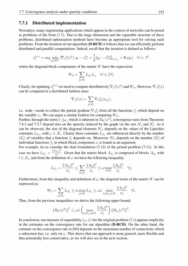
7.7 Convergence analysis under sparsity conditions 142
7.7.1 Distributed implementationNowadays, many engineering applications which appear in the context of networks can be posedas problems of the form (7.1). Due to the large dimension and the separable structure of theseproblems, distributed optimization methods have become an appropriate tool for solving suchproblems. From the iteration of our algorithm (D-RCD) it follows that we can efficiently performdistributed and parallel computations. Indeed, recall that the iteration is defined as follows:
xk+1i = arg min
yi∈Rni⟨∇if(x
k), yi − xki ⟩+1
2∥yi − xki ∥2WiiIni
+Ψi(yi) ∀i ∈ Jk,
where the diagonal block components of the matrix W have the expression:
Wii =∑j∈Ni
LNjIni
∀i ∈ [N ].
Clearly, for updating xk+1i we need to compute distributively∇if(x
k) andWii. However,∇if(x)can be computed in a distributed fashion since
∇if(x) =∑j∈Ni
∇ifj(xNj),
i.e. node i needs to collect the partial gradient ∇ifj from all the functions fj which depend onthe variable xi. We can argue a similar fashion for computing Wii.Further, through the norm ∥·∥W , which is inherent inRW (x0), convergence rates from Theorems7.4.3 and 7.5.7 depend also on the sparsity induced by the graph via the sets Nj and Ni. As itcan be observed, the size of the diagonal elements Wii depends on the values of the Lipschitzconstants LNj
, with j ∈ Ni. Clearly these constants LNjare influenced directly by the number
|Nj| of variables that a function fj depends on. Moreover, Wii depends on the number |Ni| ofindividual functions fj in which block component xi is found as an argument.For example, let us consider the dual formulation (7.12) of the primal problem (7.11). In this
case we have LNj=
∥ANj∥2
σj. Given that the matrix block ANj
is composed of blocks Alj , withl ∈ Nj , and from the definition of ω we have the following inequality:
LNj=∥ANj
∥2
σj≤∑l∈Nj
∥Alj∥2
σj≤ ωmax
l∈Nj
∥Alj∥2
σj∀j.
Furthermore, from this inequality and definition of ω, the diagonal terms of the matrix W can beexpressed as:
Wii =∑j∈Ni
LNj≤ ωmax
j∈Ni
LNj≤ ωω max
l∈Nj ,j∈Ni
∥Alj∥2
σj∀i.
Thus, from the previous inequalities we derive the following upper bound:(RW (x0)
)2 ≤ ωω
(max
l∈Nj ,j∈Ni
∥Alj∥2
σj
)(RIn(x
0))2.
In conclusion, our measure of separability (ω, ω) for the original problem (7.1) appears implicitlyin the estimates on the convergence rate for our algorithm (D-RCD). On the other hand, theestimate on the convergence rate in [94] depends on the maximum number of connections whicha subsystem has, i.e. only on ω. This shows that our approach is more general, more flexible andthus potentially less conservative, as we will also see in the next section.
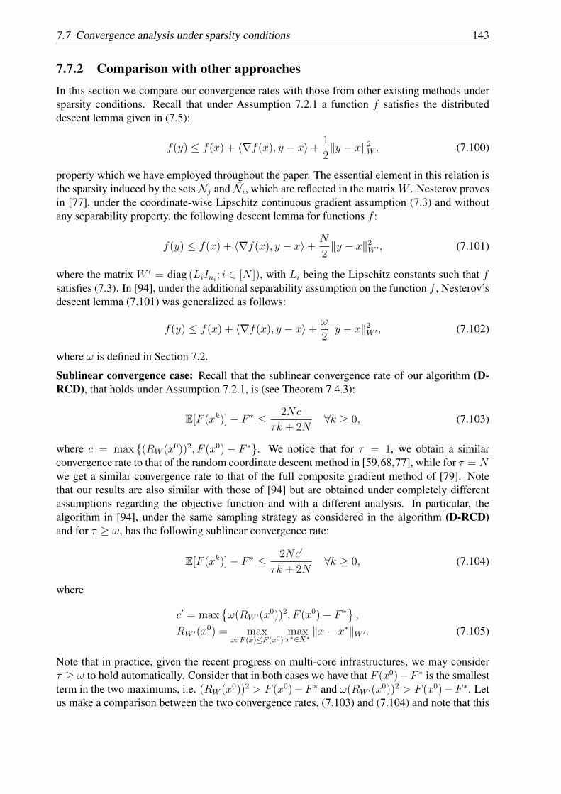
7.7 Convergence analysis under sparsity conditions 143
7.7.2 Comparison with other approachesIn this section we compare our convergence rates with those from other existing methods undersparsity conditions. Recall that under Assumption 7.2.1 a function f satisfies the distributeddescent lemma given in (7.5):
f(y) ≤ f(x) + ⟨∇f(x), y − x⟩+ 1
2∥y − x∥2W , (7.100)
property which we have employed throughout the paper. The essential element in this relation isthe sparsity induced by the setsNj and Ni, which are reflected in the matrix W . Nesterov provesin [77], under the coordinate-wise Lipschitz continuous gradient assumption (7.3) and withoutany separability property, the following descent lemma for functions f :
f(y) ≤ f(x) + ⟨∇f(x), y − x⟩+ N
2∥y − x∥2W ′ , (7.101)
where the matrix W ′ = diag (LiIni; i ∈ [N ]), with Li being the Lipschitz constants such that f
satisfies (7.3). In [94], under the additional separability assumption on the function f , Nesterov’sdescent lemma (7.101) was generalized as follows:
f(y) ≤ f(x) + ⟨∇f(x), y − x⟩+ ω
2∥y − x∥2W ′ , (7.102)
where ω is defined in Section 7.2.
Sublinear convergence case: Recall that the sublinear convergence rate of our algorithm (D-RCD), that holds under Assumption 7.2.1, is (see Theorem 7.4.3):
E[F (xk)]− F ∗ ≤ 2Nc
τk + 2N∀k ≥ 0, (7.103)
where c = max (RW (x0))2, F (x0)− F ∗. We notice that for τ = 1, we obtain a similarconvergence rate to that of the random coordinate descent method in [59,68,77], while for τ = Nwe get a similar convergence rate to that of the full composite gradient method of [79]. Notethat our results are also similar with those of [94] but are obtained under completely differentassumptions regarding the objective function and with a different analysis. In particular, thealgorithm in [94], under the same sampling strategy as considered in the algorithm (D-RCD)and for τ ≥ ω, has the following sublinear convergence rate:
E[F (xk)]− F ∗ ≤ 2Nc′
τk + 2N∀k ≥ 0, (7.104)
where
c′ = maxω(RW ′(x0))2, F (x0)− F ∗ ,
RW ′(x0) = maxx: F (x)≤F (x0)
maxx∗∈X∗
∥x− x∗∥W ′ . (7.105)
Note that in practice, given the recent progress on multi-core infrastructures, we may considerτ ≥ ω to hold automatically. Consider that in both cases we have that F (x0)−F ∗ is the smallestterm in the two maximums, i.e. (RW (x0))2 > F (x0)−F ∗ and ω(RW ′(x0))2 > F (x0)−F ∗. Letus make a comparison between the two convergence rates, (7.103) and (7.104) and note that this

7.7 Convergence analysis under sparsity conditions 144
comparison comes down to the comparison between the norms ∥ · ∥2W and ω∥ · ∥2W ′ . From thedefinitions on the norms we can express:
∥x∥2W =N∑i=1
∑j∈Ni
LNj
∥xi∥2ω∥x∥2W ′ =
N∑i=1
(ωLi)∥xi∥2.
Let us now analyze some scenarios for ω and ω defined in the upper bounding of the two normsfrom above. From Section 7.2.1 we notice that for many practical applications we have that theseLipschitz constants LNj
and Li are quite similar in size (see e.g. (7.10)). If we have that ω = 1,i.e. each function fj has only one argument, then automatically we have ω = 1, because thesubcomponent xi would appear as argument only in function fj . In this case we also have thatLi = LNi
, and the convergence rates are the same. Consider now that ω = N , i.e. we havea function fj whose argument is the entire vector x. The fact that ω = N does not imply anyassumptions on ω, apart from ω ≥ 2, due to the fact that one function has as argument the entirex. In this case, for similar Lipschitz constants Li and LNi
and for ω < N , we are superior to theconvergence rate in [94]. Finally, let us now consider that we have a very large Lipschitz constantLi, for some i ∈ [N ], as it can be found in many ill-conditioned problems from practice. In thiscase we have at most a constant LN ′
j≈ Li, for some j′ ∈ Ni. Therefore, we have the following
inequality: ∑j∈Ni
LNj≪ ωLi,
since LNj≪ Li for j ∈ Ni and j = j′. As a result, we have that (RW (x0))2 < ω(RW ′(x0))2
and the convergence rate (7.103) of (D-RCD) is better in this case than (7.104). In conclusion,the sublinear convergence rate of algorithm (D-RCD) is better than that of algorithm in [94]under similar Lipschitz constants and for ω ≪ ω ≪ n, i.e. for problems where we have atleast a function fj that depends on a large number of variables (i.e. ω relatively large) but eachvariable do not appear in many functions fj (i.e. ω relatively small). Note that this scenario wasalso considered at the beginning of the paper since coordinate gradient descent type methods forsolving problem (7.1) make sense only in the case when ω is small, otherwise incremental typemethods should be considered for solving (7.1) [114].
Linear convergence case: The authors of [59,68,77,94] provide also linear convergence rate fortheir algorithms. A straightforward comparison between convergence rates in this case cannotbe done, due to the fact the linear convergence in [59, 68, 77, 94] is proved under the moreconservative assumption of strong convexity, while the convergence rate of our algorithm (D-RCD) is obtained under the more relaxed assumption of generalized error bound property (7.40)given in Definition 7.5.1. However, we can also consider f to be strongly convex with a constantσW w.r.t. the norm ∥ · ∥W . From Section 7.6.1 it follows that strongly convex functions areincluded in our class of generalized error bound functions (7.40) with κ1 = 2
σWand κ2 = 0. In
this case we have the following linear convergence of algorithm (D-RCD) (see Theorem 7.5.7):
E[F (xk+1)− F ∗] ≤ (1− γebsc)k
(F (x0)− F ∗) , (7.106)
where γebsc =τσW
4√Nτ+4N+σW (2N−τ)
. Now, if we consider f to be strongly convex in the norm ∥·∥W ′
with a constant σW ′ , then the algorithm in [94] has a convergence rate:
E[F (xk+1)− F ∗] ≤ (1− γsc)k
(F (x0)− F ∗) , (7.107)
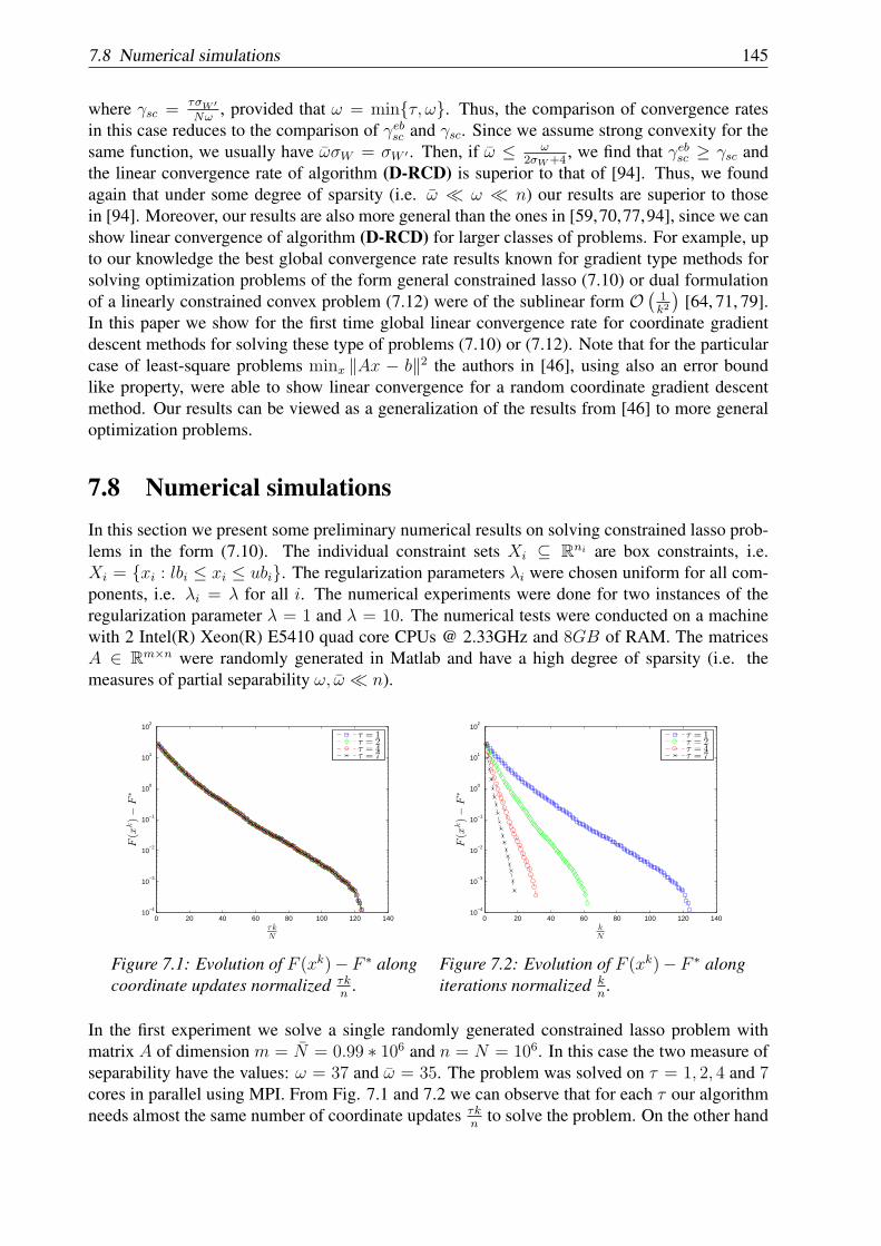
7.8 Numerical simulations 145
where γsc =τσW ′Nω
, provided that ω = minτ, ω. Thus, the comparison of convergence ratesin this case reduces to the comparison of γebsc and γsc. Since we assume strong convexity for thesame function, we usually have ωσW = σW ′ . Then, if ω ≤ ω
2σW+4, we find that γebsc ≥ γsc and
the linear convergence rate of algorithm (D-RCD) is superior to that of [94]. Thus, we foundagain that under some degree of sparsity (i.e. ω ≪ ω ≪ n) our results are superior to thosein [94]. Moreover, our results are also more general than the ones in [59,70,77,94], since we canshow linear convergence of algorithm (D-RCD) for larger classes of problems. For example, upto our knowledge the best global convergence rate results known for gradient type methods forsolving optimization problems of the form general constrained lasso (7.10) or dual formulationof a linearly constrained convex problem (7.12) were of the sublinear form O
(1k2
)[64, 71, 79].
In this paper we show for the first time global linear convergence rate for coordinate gradientdescent methods for solving these type of problems (7.10) or (7.12). Note that for the particularcase of least-square problems minx ∥Ax − b∥2 the authors in [46], using also an error boundlike property, were able to show linear convergence for a random coordinate gradient descentmethod. Our results can be viewed as a generalization of the results from [46] to more generaloptimization problems.
7.8 Numerical simulationsIn this section we present some preliminary numerical results on solving constrained lasso prob-lems in the form (7.10). The individual constraint sets Xi ⊆ Rni are box constraints, i.e.Xi = xi : lbi ≤ xi ≤ ubi. The regularization parameters λi were chosen uniform for all com-ponents, i.e. λi = λ for all i. The numerical experiments were done for two instances of theregularization parameter λ = 1 and λ = 10. The numerical tests were conducted on a machinewith 2 Intel(R) Xeon(R) E5410 quad core CPUs @ 2.33GHz and 8GB of RAM. The matricesA ∈ Rm×n were randomly generated in Matlab and have a high degree of sparsity (i.e. themeasures of partial separability ω, ω ≪ n).
0 20 40 60 80 100 120 14010
−4
10−3
10−2
10−1
100
101
102
τk
N
F(x
k)−
F∗
τ = 1τ = 2τ = 4τ = 7
Figure 7.1: Evolution of F (xk)− F ∗ alongcoordinate updates normalized τk
n.
0 20 40 60 80 100 120 14010
−4
10−3
10−2
10−1
100
101
102
k
N
F(x
k)−
F∗
τ = 1τ = 2τ = 4τ = 7
Figure 7.2: Evolution of F (xk)− F ∗ alongiterations normalized k
n.
In the first experiment we solve a single randomly generated constrained lasso problem withmatrix A of dimension m = N = 0.99 ∗ 106 and n = N = 106. In this case the two measure ofseparability have the values: ω = 37 and ω = 35. The problem was solved on τ = 1, 2, 4 and 7cores in parallel using MPI. From Fig. 7.1 and 7.2 we can observe that for each τ our algorithmneeds almost the same number of coordinate updates τk
nto solve the problem. On the other hand
7.8 Numerical simulations 146
0 5 10 15 20 25 3010
−4
10−3
10−2
10−1
100
101
102
sF(x
k)−
F∗
τ = 1τ = 2τ = 4τ = 7
Figure 7.3: Evolution of F (xk)− F ∗ along computational time.
increasing the number of cores reduces substantially the number of iterations kn
. In Fig. 7.3 weplot the decrease of the objective function along the computational time for τ = 1, 2, 4 and 7cores.In the second set of experiments, provided in Table 7.1, the dimension of matrix A ranges asfollows: m = N from 0.9 ∗ 104 to 1.1 ∗ 106 and n = N from 104 to 106. For the resultingproblem our objective function satisfies the generalized error bound property (7.40) given inDefinition 7.5.1 and in some cases it is even strongly convex. This series of numerical testswere undertaken in order to compare the full number of iterations of algorithm (D-RCD) againstalgorithm (PCDM1) in [94] with β = min ω, τ (since for this choice of β the authors in [94]were able to prove sublinear convergence rate for their algorithm). In these simulations thealgorithms were implemented in a centralized manner, i.e. there is no inter-core transmissionof data, with the number of updates per iteration of τ = 100 in each case. Both algorithmswere allowed to reach the same optimal value F ∗ which is presented in the last column andwas computed with the serial (τ = 1) random coordinate descent method. The second andthird column of the table represent the dimensions of matrix A. The fourth column representsthe degree of sparsity which dictates that the total number of nonzero elements in the matrixA is less than or equal to n × m × sparse. The fifth and sixth columns denote the degrees ofpartial separability ω and ω, while the seventh and eighth columns represent the total numberof coordinate updates normalized that the algorithms completed. As it can be observed fromTable 7.1, algorithm (D-RCD) outperforms (PCDM1) even in the case where ω and ω are ofsimilar size or equal. Moreover, note that between the problems where m is slightly larger thann, i.e. where the resulting objective function F (x) is strongly convex, and the problems wherem is slightly smaller than n, i.e. where F (x) is not strongly convex but satisfies our generalizederror bound property (7.40), the number of iterations of algorithm (D-RCD) is comparable. Inconclusion, given that the constrained lasso problems of the form (7.10) satisfy the generalizederror bound property (7.40), the theoretical result that linear convergence of algorithm (D-RCD)is attained under the generalized error bound property is confirmed also in practice.
A comparison of the decrease of the objective function for both algorithms on a randomlygenerated lasso problem with dimensions n = 105 and m = 0.985 × 10⁵ of matrix A is plottedin semilogarithmic scale in Fig. 7.4.
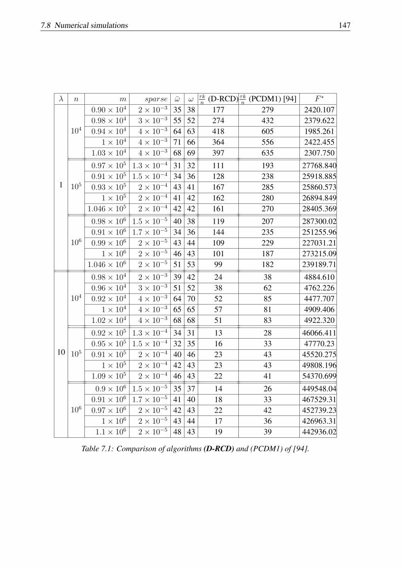
7.8 Numerical simulations 147
λ n m sparse ω ω τkn
(D-RCD) τkn
(PCDM1) [94] F ∗
1
104
0.90× 10⁴ 2× 10⁻³ 35 38 177 279 2420.1070.98× 104 3× 10⁻³ 55 52 274 432 2379.6220.94× 104 4× 10⁻³ 64 63 418 605 1985.261
1× 10⁴ 4× 10⁻³ 71 66 364 556 2422.4551.03× 104 4× 10⁻³ 68 69 397 635 2307.750
105
0.97× 10⁵ 1.3× 10⁻⁴ 31 32 111 193 27768.8400.91× 105 1.5× 10⁻⁴ 34 36 128 238 25918.8850.93× 105 2× 10⁻⁴ 43 41 167 285 25860.573
1× 10⁵ 2× 10⁻⁴ 41 42 162 280 26894.8491.046× 105 2× 10⁻⁴ 42 42 161 270 28405.369
106
0.98× 10⁶ 1.5× 10⁻⁵ 40 38 119 207 287300.020.91× 106 1.7× 10⁻⁵ 34 36 144 235 251255.960.99× 106 2× 10⁻⁵ 43 44 109 229 227031.21
1× 10⁶ 2× 10⁻⁵ 46 43 101 187 273215.091.046× 106 2× 10⁻⁵ 51 53 99 182 239189.71
10
104
0.98× 10⁴ 2× 10⁻³ 39 42 24 38 4884.6100.96× 104 3× 10⁻³ 51 52 38 62 4762.2260.92× 104 4× 10⁻³ 64 70 52 85 4477.707
1× 10⁴ 4× 10⁻³ 65 65 57 81 4909.4061.02× 104 4× 10⁻³ 68 68 51 83 4922.320
105
0.92× 10⁵ 1.3× 10⁻⁴ 34 31 13 28 46066.4110.95× 105 1.5× 10⁻⁴ 32 35 16 33 47770.230.91× 105 2× 10⁻⁴ 40 46 23 43 45520.275
1× 10⁵ 2× 10⁻⁴ 42 43 23 43 49808.1961.09× 105 2× 10⁻⁴ 46 43 22 41 54370.699
106
0.9× 10⁶ 1.5× 10⁻⁵ 35 37 14 26 449548.040.91× 106 1.7× 10⁻⁵ 41 40 18 33 467529.310.97× 106 2× 10⁻⁵ 42 43 22 42 452739.23
1× 10⁶ 2× 10⁻⁵ 43 44 17 36 426963.311.1× 106 2× 10⁻⁵ 48 43 19 39 442936.02
Table 7.1: Comparison of algorithms (D-RCD) and (PCDM1) of [94].
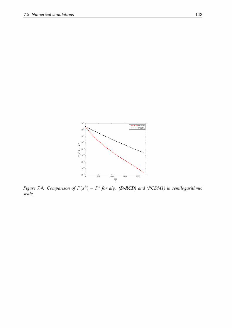
7.8 Numerical simulations 148
0 500 1000 1500 200010
−5
10−4
10−3
10−2
10−1
100
101
102
103
τk
n
F(x
k)−
F∗
D−RCDPCDM1
Figure 7.4: Comparison of F (xk) − F ∗ for alg. (D-RCD) and (PCDM1) in semilogarithmicscale.
Chapter 8
Parallel coordinate descent algorithm forseparable constraints optimization:application to MPC
In this chapter we propose a parallel coordinate descent algorithm for solving smooth convex op-timization problems with separable constraints that may arise e.g. in distributed model predictivecontrol (MPC) for linear networked systems. Our algorithm is based on block coordinate descentupdates in parallel and has a very simple iteration. We prove (sub)linear rate of convergence forthe new algorithm under standard assumptions for smooth convex optimization. Further, our al-gorithm uses local information and thus is suitable for distributed implementations. Moreover, ithas low iteration complexity, which makes it appropriate for embedded control. An MPC schemebased on this new parallel algorithm is derived, for which every subsystem in the network cancompute feasible and stabilizing control inputs using distributed and cheap computations. Forensuring stability of the MPC scheme, we use a terminal cost formulation derived from a dis-tributed synthesis. Preliminary numerical tests show better performance for our optimizationalgorithm than other existing methods. This chapter is based on paper [61].
8.1 IntroductionModel predictive control (MPC) has become a popular advanced control technology imple-mented in networked systems due to its ability to handle hard input and state constraints [92].Network systems are usually modeled by a graph whose nodes represent subsystems and whosearcs indicate dynamic couplings. These types of systems are complex and large in dimension,whose structures may be hierarchical and they have multiple decision-makers (e.g. process con-trol [65], traffic and power systems [112]).Decomposition methods represent a very powerful tool for solving distributed MPC problemsin networked systems. The basic idea of these methods is to decompose the original large op-timization problem into smaller subproblems. Decomposition methods can be divided in twomain classes: primal and dual decomposition methods. In primal decomposition the optimiza-tion problem is solved using the original formulation and variables via methods such as interior-point, feasible directions, Gauss-Jacobi type and others [13,27,103,112]. In dual decompositionthe original problem is rewritten using Lagrangian relaxation for the coupling constraints and thedual problem is solved with a Newton or (sub)gradient algorithm [1,9,62,65]. In [103,112] coop-erative based distributed MPC algorithms are proposed based on Gauss-Jacobi iterations, where
149
8.1 Introduction 150
asymptotic convergence to the centralized solution and feasibility for their iterates is proved.In [27] non-cooperative algorithms are derived for distributed MPC problems, where commu-nication takes place only between neighbors. In [13] a distributed algorithm based on interior-point methods is proposed whose iterates converge to the centralized solution. In [1,62,65] dualdistributed gradient algorithms based on Lagrange relaxation of the coupling constraints are pre-sented for solving MPC problems, algorithms which usually produce feasible and optimal primalsolutions in the limit. While much research has focused on a dual approach, our work developsa primal method that ensures constraint feasibility, has low iteration complexity and providesestimates on suboptimality.Further, MPC schemes tend to be quite costly computation-wise compared with classical controlmethods, e.g. PID controllers, so that for these advanced schemes we need hardware with a rea-sonable amount of computational power that is embedded on the subsystems. Therefore, researchfor distributed and embedded MPC has gained momentum in the past few years. The conceptbehind embedded MPC is designing a control scheme that can be implemented on autonomouselectronic hardware, e.g programmable logic controllers (PLC) or field-programmable gate ar-rays (FPGAs) [37]. Such devices vary widely in both computational power and memory storagecapabilities as well as cost. As a result, there has been a growing focus on making MPC schemesfaster by reducing problem size and improving the computational efficiency through decentral-ization [62, 65], moving block strategies (e.g. by using latent variables or Laguerre functions)and other procedures, allowing these schemes to be implemented on cheaper hardware with littlecomputational power.The main contribution of this chapter is the development of a parallel coordinate descent algo-rithm for smooth convex optimization problems with separable constraints that is computation-ally efficient and thus suitable for MPC schemes that need to be implemented distributively or inhardware with limited computational power. This algorithm employs parallel block-coordinateupdates for the optimization variables and has similarities to the optimization algorithm proposedin [103], but with simpler implementation, lower iteration complexity and guaranteed rate of con-vergence. We derive (sub)linear rate of convergence for the new algorithm whose proof relieson the Lipschitz property of the gradient of the objective function. The new parallel algorithmis used for solving MPC problems for general linear networked systems in a distributed fash-ion using local information. For ensuring stability of the MPC scheme, we use a terminal costformulation derived from a distributed synthesis and we eliminate the need for a terminal stateconstraint. Compared with the existing approaches based on an end point constraint, we reducethe conservatism by combining the underlying structure of the system with distributed optimiza-tion [33, 48]. Because the MPC optimization problem is usually terminated before convergence,our MPC controller is a form of suboptimal control. However, using the theory of suboptimalcontrol [102] we can still guarantee feasibility and stability.This chapter is organized as follows. In Section 8.2 we derive our parallel coordinate descentoptimization algorithm and prove the convergence rate for it. In Section 8.3 we introduce themodel for general networked systems, present the MPC problem with a terminal cost formula-tion and provide the means for which this terminal cost can be synthesized distributively. InSection 8.4 we employ our algorithm for distributively solving MPC problems arising from net-worked systems and discuss details regarding its implementation. In Section 8.5 we compareits performance with other algorithms and test it on a real application - a quadruple water tankprocess.
8.2 Parallel coordinate descent algorithm (PCDM) for separable constraints minimization 151
8.2 Parallel coordinate descent algorithm (PCDM) for sepa-rable constraints minimization
We work in Rn composed by column vectors. For u, v ∈ Rn we denote the standard Euclideaninner product ⟨u, v⟩ = uTv, the Euclidean norm ∥u∥ =
√⟨u, u⟩ and ∥x∥2P = xTPx. Further, for
a symmetric matrix P , we use P ≻ 0 (P ≽ 0) for a positive (semi)definite matrix. For matricesP and Q, we use diag(P,Q) to denote the block diagonal matrix formed by these two matrices.In this section we propose a parallel coordinate descent based algorithm for efficiently solvingthe general convex optimization problem of the following form:
f ∗ = minu1∈U1,··· ,uM∈UM
f(u1, . . . ,uM), (8.1)
where ui ∈ Rniu with i = 1, . . . ,M , are the decision variables, constrained to individual convex
sets Ui ⊂ Rniu . We gather the individual constraint sets Ui into the set U = U1 × · · · ×UM ,
and denote the entire decision variable for (8.1) by u =[(u1)T . . . (uM)T
]T ∈ Rnu , withnu =
∑Mi=1 n
iu. As we will show in this section, the new algorithm can be used on many
parallel computing architectures, has low computational cost per iteration and guaranteed con-vergence rate. We will then apply this algorithm for solving distributed MPC problems arisingin networked systems in Section 8.3.
8.2.1 Parallel Block-Coordinate Descent MethodLet us partition the identity matrix in accordance with the structure of the decision variable u:
Inu =[(E1)T . . . (EM)T
]T ∈ Rnu×nu ,
where Ei ∈ Rnu×niu for all i = 1, · · · ,M . With matrices Ei we can represent u =
∑Mi=1E
iui.We also define the partial gradient ∇if(u) ∈ Rni
u of f(u) as: ∇if(u) = (Ei)T∇f(u). Weassume that the gradient of f is coordinate-wise Lipschitz continuous with constants Li > 0, i.e:∥∥∇if(u+ Eihi)−∇if(u)
∥∥ ≤ Li ∥hi∥ ∀u ∈ Rnu , hi ∈ Rniu . (8.2)
Due to the assumption that f is coordinate-wise Lipschitz continuous, it can be easily deducedthat [76]:
f(u+ Eihi) ≤ f(u) + ⟨∇if(u), hi⟩+Li
2∥hi∥2 ∀u ∈ Rnu , hi ∈ Rni
u . (8.3)
We now introduce the following norm for the extended space Rnu:
∥u∥21 =M∑i=1
Li
∥∥ui∥∥2 , (8.4)
which will prove useful for estimating the rate of convergence for our algorithm. Additionally, iffunction f is smooth and strongly convex with regards to ∥·∥1 with a parameter σ1, then [75]:
f(w) ≥ f(v) + ⟨∇f(v),w − v⟩+ σ12∥w − v∥21 ∀w,v ∈ Rnu . (8.5)
8.2 Parallel coordinate descent algorithm (PCDM) for separable constraints minimization 152
Note that if f is strongly convex w.r.t the standard Euclidean norm ∥·∥ with a parameter σ0, thenσ0 ≥ σ1L
imax, where Li
max = maxiLi. By taking w = v + Eihi and v = u in (8.5) we also get:
f(u+ Eihi) ≥ f(u) + ⟨∇if(u), hi⟩+σ1Li
2∥hi∥2 ∀u ∈ Rnu , hi ∈ Rni
u ,
and combining with (8.3) we also deduce that σ1 ≤ 1.We now define the constrained coordinate update for our algorithm:
vi(u) = arg minvi∈Ui
⟨∇if(u),v
i − ui⟩+Li
2
∥∥vi − ui∥∥2
ui(u) = u+ Ei(vi(u)− ui), i = 1, . . . ,M.
The optimality conditions for the previous optimization problem are:⟨∇if(u) + Li(v
i(u)− ui),vi − vi(u)⟩≥ 0 ∀vi ∈ Ui. (8.6)
Taking vi = ui in the previous inequality and combining with (8.3) we obtain the followingdecrease in the objective function:
f(u)− f(ui(u)) ≥ Li
2
∥∥vi(u)− ui∥∥2 . (8.7)
We now present our Parallel Coordinate Descent Method, that resembles the method in [103] butwith simpler implementation, lower iteration complexity and guaranteed rate of convergence, andis a parallel version of the coordinate descent method from [76]:
Algorithm PCDM
Choose ui0 ∈ Ui for all i = 1, . . . ,M . For
k ≥ 0:
1. Compute in parallel vi(uk), i =1, . . . ,M.
2. Update in parallel:
uik+1 =
1
Mvi(uk)+
M − 1
Muik, i = 1, . . . ,M.
Note that if the sets Ui are simple (by simple we understand that the projection on thesesets is easy), then computing vi(u) consists of projecting a vector on these sets and can bedone numerically very efficient. For example, if these sets are simple box sets, i.e Ui =ui ∈ Rni
u|uimin ≤ ui ≤ ui
max
, then the complexity of computing vi(u), once∇if(u) is avail-
able, is O(niu). In turn, computing ∇if(u) has, in the worst case, complexity O(ni
unu) forquadratic dense functions. Thus, Algorithm PCDM has usually a very low iteration cost per sub-system compared to other existing methods, e.g. Jacobi type algorithm presented in [103], whichusually require numerical complexity at least O((ni
u)3 + ni
unu) per iteration for each subsystemi, provided that the local quadratic problems are solved with an interior point solver. Also, in the
8.2 Parallel coordinate descent algorithm (PCDM) for separable constraints minimization 153
following two theorems we provide estimates for the convergence rate of our algorithm, whilefor the algorithm in [103] only asymptotic convergence is proved.From (8.6)-(8.7), convexity of f and uk+1 =
∑i
1Mui(uk) we see immediately that method
PCDM decreases strictly the objective function at each iteration, provided that uk = u∗, whereu∗ is the optimal solution of (8.1), i.e.:
f(uk+1) < f(uk) ∀k ≥ 0, uk = u∗. (8.8)
Let f ∗ be the optimal value in optimization problem (8.1). The following theorem derives conver-gence rate of Algorithm PCDM and employs standard techniques for proving rate of convergenceof the gradient method [75, 76]:
Theorem 8.2.1 If function f in optimization problem (8.1) has a coordinate-wise Lipschitz con-tinuous gradient with constants Li as given in (8.2), then Algorithm PCDM has the followingsublinear rate of convergence:
f(uk)−f ∗ ≤ M
M + k
(1
2r20 + f(u0)−f ∗
),
where r0 = ∥u0−u∗∥1.
Proof : We introduce the following term:
r2k = ∥uk−u∗∥21 =M∑i=1
Li
⟨uik−ui
∗,uik−ui
∗⟩,
where u∗ is the optimal solution of (8.1) and ui∗ = (Ei)Tu∗. Then, using similar derivations as
in [76], we have:
r2k+1=M∑i=1
Li
∥∥∥∥ 1
Mvi(uk) + (1− 1
M)ui
k−ui∗
∥∥∥∥2(8.6)≤ r2k +
M∑i=1
Li
M(1
M−2)
∥∥vi(uk)− uik
∥∥2 + 2
M
⟨∇if(uk),u
i∗−vi(uk)
⟩1M
≤1
≤ r2k −2
M
M∑i=1
(Li
2
∥∥vi(uk)− uik
∥∥2 +⟨∇if(uk), v
i(uk)− uik
⟩+⟨∇if(uk),u
i∗−ui
k
⟩).
By convexity of f and (8.3) we obtain:
r2k+1 ≤ r2k−2(f(uk+1)− f(uk)) +2
M⟨∇f(uk),u∗ − uk⟩ (8.9)
and adding up these inequalities we get:
1
2r20+f(u0)−f ∗≥ 1
2r2k+1+f(uk+1)−f ∗+
1
M
k∑j=0
(f(uj)−f ∗)
≥ f(uk+1)−f ∗ +1
M
k∑j=0
(f(uj)−f ∗).
Taking into account that our algorithm is a descent algorithm, i.e. f(uj) ≥ f(uk+1) for all j ≤ kand by the previous inequality the proof is complete. 2
8.3 Application of PCDM to distributed suboptimal MPC 154
Now, we derive linear convergence rate for Algorithm PCDM, provided that f is additionallystrongly convex:
Theorem 8.2.2 Under the assumptions of Theorem 8.2.1 and if we further assume that f isstrongly convex with regards to ∥·∥1 with a constant σ1 as given in (8.5), then the followinglinear rate of convergence is achieved for Algorithm PCDM:
f(uk)−f ∗≤(1− 2σ1
M(1 + σ1)
)k(1
2r20+f(u0)−f ∗
).
Proof : We take w = u∗ and v = uk in (8.5) and through (8.9) we get:
1
2r2k+1 + f(uk+1)− f ∗ ≤1
2r2k + f(uk)− f ∗ − 1
M(f(uk)− f ∗ +
σ12r2k). (8.10)
From the strong convexity of f in (8.5) we also get:
f(uk)− f ∗ +σ12r2k ≥ σ1r
2k.
We now define γ = 2σ1
1+σ1∈ [0, 1] and using the previous inequality we obtain the following
result:
f(uk)− f ∗ +σ12r2k ≥γ
(f(uk)− f ∗ +
σ12r2k
)+ (1− γ)σ1r2k.
Using this inequality in (8.10) we get:
1
2r2k+1+f(uk+1)− f ∗≤
(1− γ
M
)(1
2r2k + f(uk)− f ∗
).
Applying this inequality iteratively, we obtain the following for k ≥ 0:
1
2r2k+f(uk)−f ∗≤
(1− γ
M
)k (1
2r20 + f(u0)− f ∗
),
and by replacing γ = 2σ1
1+σ1we complete the proof. 2
The following properties follow immediately for our Algorithm PCDM.
Lemma 8.2.3 For the optimization problem (8.1), with the assumptions of Theorem 8.2.2, wehave the following statements:(i) Given any feasible initial guess u0, the iterates of the Algorithm PCDM are feasible at eachiteration, i.e. ui
k ∈ Ui for all k ≥ 0.(ii) The function f is nonincreasing, i.e. f(uk+1) ≤ f(uk) according to (8.8).(iii) The sub(linear) rate of convergence of Algorithm PCDM is given in Theorem 8.2.1 (Theorem8.2.2).
8.3 Application of PCDM to distributed suboptimal MPCThe Algorithm PCDM can be used to solve distributively input constrained MPC problems fornetworked systems after state elimination. In this section we show that the MPC scheme obtainedby solving approximately the corresponding optimization problem with Algorithm PCDM isstable and distributed.
8.3 Application of PCDM to distributed suboptimal MPC 155
8.3.1 MPC for networked systems: terminal cost and no end constraintsIn this chapter we consider discrete-time networked systems, which are usually modeled by agraph whose nodes represent subsystems and whose arcs indicate dynamic couplings, defined bythe following linear state equations [13, 65]:
xit+1 =∑j∈N i
Aijxjt +Bijujt , i = 1, · · · ,M, (8.11)
where M denotes the number of interconnected subsystems, xjt ∈ Rnj and ujt ∈ Rmj representthe state and respectively the input of jth subsystem at time t, Aij ∈ Rni×nj , Bij ∈ Rni×mj andN i is the set of indices which contains the index i and that of its neighboring subsystems. Aparticular case of (8.11), that is frequently found in literature [62, 103, 112], has the followingdynamics:
xit+1 = Aiixit +∑j∈N i
Bijujt . (8.12)
For stability analysis, we also express the dynamics of the entire system: xt+1 = Axt + But,
where n =M∑i=1
ni, m =M∑i=1
mi, xt ∈ Rn, ut ∈ Rm and A ∈ Rn×n, B ∈ Rn×m. For system
(8.11) or (8.12) we consider local input constraints:
uit ∈ U i i = 1, · · · ,M, t ≥ 0, (8.13)
with U i ⊆ Rmi compact, convex sets with the origin in their interior. We also consider convexlocal stage and terminal costs for each subsystem i: ℓi(xi, ui) and ℓif(x
i). Let us denote the inputtrajectory for subsystem i and the overall input trajectory for the entire system by:
ui = [(ui0)T · · · (uiN−1)
T ]T , u = [(u1)T · · · (uM)T ]T .
We can now formulate the MPC problem for system (8.11) over a prediction horizon of lengthN and a given initial state x as [92]:
V ∗N(x) = min
uit∈U i ∀i,t
VN(x,u)
(:=
M∑i=1
N−1∑t=0
ℓi(xit, uit) + ℓif(x
iN)
)(8.14)
s.t: xit+1 =∑j∈N i
Aijxjt +Bijujt , xi0 = xi, i = 1, · · · ,M, t ≥ 0.
It is well-known that by eliminating the states using dynamics (8.11), the MPC problem (8.14)can be recast [92] as a convex optimization problem of type (8.1), where ni
u = Nmi, the func-tion f is convex (recall that we assume the stage and final costs ℓi(·) and ℓif(·) to be convex),whilst the convex sets Ui are the Cartesian product of the convex sets U i for N times. We de-note the approximate solution produced by Algorithm PCDM for problem (8.14) after certainnumber of iterations with uCD. We also consider that at each MPC step the Algorithm PCDMis initialized (warm start) with the shifted sequence of controllers obtained at the previous stepand the feedback controller κ(·) computed in Section 8.3.2 below. The suboptimal MPC schemecorresponding to (8.14) would now be:

8.3 Application of PCDM to distributed suboptimal MPC 156
Suboptimal MPC scheme
Given initial state x and initial uCD repeat:
1. Recast MPC problem (8.14) as opt. problem(8.1)
2. Solve (8.1) approximately with Alg. PCDMstarting from uCD and obtain uCD
3. Update x. Update uCD using warm start.
8.3.2 Distributed synthesis for a terminal costWe assume that stability of the MPC scheme (8.14) is enforced by adapting the terminal costℓf(·) =
∑Mi=1 ℓ
if(·) and the horizon lengthN appropriately such that sufficient stability criteria are
fulfilled [33,48]. Usually, stability of MPC with quadratic stage cost ℓi(xi, ui) = ∥xi∥2Qi+∥ui∥2Ri ,where the matrices Qi ≽ 0 and Ri ≻ 0, and without terminal constraint is enforced if thefollowing criteria hold: there exists a neighborhood of the origin Ω ⊆ Rn, a stabilizing feedbacklaw κ(·) and a terminal cost ℓf(·) such that we have
ℓf(Ax+Bκ(x))− ℓf(x) + κ(x)TRκ(x) + xTQx ≤ 0 ∀x ∈ Ω
κ(x) ∈ U, Ax+Bκ(x) ∈ Ω,(8.15)
where the matrices Q and R have a block diagonal structure and are composed of the blocksQi and Ri, respectively. As shown in [33, 48], MPC schemes based on the condition (8.15)are usually less conservative than schemes based on end point constraint. Keeping in line withthe distributed nature of our system, the control law κ(·) and the final stage cost ℓf(·) need tobe computed locally. In this section we develop a distributed synthesis procedure to constructthem locally. We choose the terminal cost for each subsystem i to be quadratic: ℓif(x
iN) =
∥xiN∥2
P i , where P i ≻ 0. For a locally computed κ(·), we employ distributed control laws: ui =F ixi, i.e. κ(·) is taken linear with a block-diagonal structure. Centralized LMI formulations of(8.15) for quadratic terminal costs are well-known in the literature [92]. However, our goal isto solve (8.15) distributively. To this purpose, we first need to introduce vectors xN i ∈ RnN i
and uN i ∈ RmN i for subsystem i, where nN i =∑j∈N i
nj and mN i =∑j∈N i
mj . These vectors
are comprised of the state and input vectors of subsystem i and those of its neighbors: xN i=[
(xj)T , j ∈ N i]T, uN
i=[(uj)T , j ∈ N i
]T.
Since our synthesis procedure needs to be distributed and taking into account that ℓf(·) =∑Mi=1 ℓ
if(·), we impose the following distributed structure to ensure (8.15) (see also [38] for a
similar approach where infinity-norm control Lyapunov functions are synthesized in a decentral-ized fashion by solving linear programs for each subsystem) for i = 1, · · · ,M :
ℓif((xi)+)−ℓif((xi))+(F ixi)TRiF ixi+(xi)TQixi ≤ qi(xN
i
) ∀xN i∈ RnN i (8.16)
such that q(x) =∑M
i=1 qi(xN
i) ≤ 0. We assume that qi(xN i
) also have a quadratic form, with
qi(xNi) =
∥∥∥xN i∥∥∥2WN i
, where WN i ∈ RnN i×nN i . Being a sum of quadratic functions, q(x) can
8.3 Application of PCDM to distributed suboptimal MPC 157
itself be expressed as a quadratic function, q(x) = ∥x∥2W , where W ∈ Rn×n is formed from theappropriate block components of matrices WN i . Note that we do not require that matrices WN i
be negative semidefinite. On the contrary, positive or indefinite matrices allow local terminalcosts to increase so long as the global cost still decreases. This approach reduces the conservatismin deriving the matrices P i and F i. For obtaining P i and F i, we introduce matrices Ei
n ∈ Rni×n,Ei
m ∈ Rmi×m, JN i
n ∈ RnN i×n, JN i
m ∈ RmN i×m such that xi = Einx, u
i = Eimu, x
N i= JN i
n xand uN
i= JN i
m u. We now define the matrices AN i= Ei
nA(JN i
n )T , BN i= Ei
nB(JN i
m )T
and FN i= JN i
m F (JN i
n )T , as to express the dynamics (8.11) for subsystem i: xit+1 = (AN i+
BN iFN i
)xNi
t . Using these notations we can now recast inequality (8.16) as:
(AN i
+BN i
FN i
)TP i(AN i
+BN i
FN i
) (8.17)
− JN i
n (Ein)
T (P i +Qi + (F i)TRiF i)Ein(J
N i
n )T ≼ WN i
.
The task of finding suitable P i, F i and WN i matrices is now reduced to the following optimiza-tion problem:
minP i,F i,WN i
,δδ : MI (8.17), i = 1, · · · ,M, W ≼ δI. (8.18)
It can be easily observed that if the optimal value δ∗ ≤ 0, consequently W ≤ 0 and (8.15) holds.This optimization problem, in its current nonconvex form, cannot be solved efficiently. However,it can be recast as a sparse SDP if we can reformulate (8.17) as an LMI. We need now to makethe assumption that all the subsystems have the same dimension for the states, i.e. ni = nj forall i, j. Subsequently, we introduce the well-known linearizations: P i = (Si)−1, F i = Y iG−1
and a series of matrices that will be of aid in formulating the LMIs:
GN i
= I|N i| ⊗G, GN i\i = [0 I|N i|−1 ⊗G], SN i
= diag(Si, µiI(nN i−ni))
Y i,j=F jG, j ∈ N i\i, Y N i
=diag(Y i,Y i,j)=FN i
GN i
,
TN i
=
[AN i
GN i+BN i
Y N i
GN i\i
], T i=
[(Qi)
12G 0
(Ri)12Y i 0
],
where the 0 blocks are of appropriate dimensions1.
Lemma 8.3.1 If the following SDP:
minG,Si,Y i,Y i,j ,W ,µi,δ
δ (8.19)
s.t:
GN i+(GN i
)T−SN i+WN i ∗ ∗
TN iSN i∗
T i 0 I
≻ 0 (8.20)
Y i,j = Y j ∀j ∈ N i, i = 1, · · · ,M, W ≼ δI,
has an optimal value δ∗ ≤ 0, then (8.15) holds2.
1By In we denote the identity matrix of size n×n, by⊗ we denote the standard Kronecker product and by∣∣N i
∣∣the cardinality of the set N i.
2By ∗ we denote the transpose of the symmetric block of the matrix.
8.4 Distributed implementation of MPC scheme based on PCDM 158
Proof : From (8.20) we observe that SN i ≻ 0, so that (SN i −GN i)T (SN i
)−1(SN i
−GN i) ≽ 0, which in turn implies
GN i
+ (GN i
)T − SN i ≼ (GN i
)T (SN i
)−1GN i
. (8.21)
If we apply the Schur complement to (8.20), we obtain:
0 ≼GN i
+ (GN i
)T − SN i
+ WN i − (TN i
)T (SN i
)−1TN i − (T i)TT i
and by (8.21) we get (GN i)−T
[(TN i
)T (SN i)−1TN i
+ (T i)TT i](GN i
)−1 − (SN i)−1
≼ (GN i)−T WN i
(GN i)−1, which is equivalent to (8.17) if we consider WN i
=(GN i
)−T WN i(GN i
)−1. 2
There exist in literature many optimization algorithms (see e.g. [57]) for solving distributivelysparse SDP problems in the form (8.19).
8.3.3 Stability of the MPC schemeWe can consider the cost function of the MPC problem VN(x,u
CD) as a Lyapunov function, usingthe standard theory for suboptimal control (see e.g. [48,92,102,103] for similar approaches). Wealso consider that at each MPC step the Algorithm PCDM is initialized (warm start) with theshifted sequence of controllers obtained at the previous step and the feedback controller κ(·)computed in Section 8.3.2 such that (8.15) is satisfied and we denote it by (uCD)+. Assume alsothat κ(·), ℓf (·) and α > 0 are chosen such that, together with the following set
Ω = x ∈ Rn : ℓf (x) ≤ α ,
satisfies (8.15). Then, using Theorem 3 from [48] we have that our MPC controller stabilizesasymptotically the system for all initial states x ∈ XN , where
XN = x ∈ Rn : V ∗N(x) ≤ Nd+ α ,
such that VN(x,uCD) ≤ Nd+ α, where d > 0 is a parameter for which we have ℓ(x,u) ≥ d forall x /∈ Ω. Clearly, this MPC scheme is locally stable with a region of attraction XN .
8.4 Distributed implementation of MPC scheme based onPCDM
In this section we discuss some technical aspects for the distributed implementation of the MPCscheme derived above when using Algorithm PCDM to solve the control problem (8.14). Usu-ally, in the linear MPC framework, the local stage and final cost are taken of the followingquadratic form:
ℓi(xi, ui) =∥∥xi∥∥2
Qi +∥∥ui∥∥2
Ri , ℓif(xi) =
∥∥xi∥∥2P i ,
where the matrices Qi, P i ∈ Rni×ni are positive semidefinite, whilst matrices Ri ∈ Rmi×mi
are positive definite. We also assume that the local constraints sets U i are polyhedral. In this
8.5 Numerical Results 159
particular case, the objective function in (8.14), after eliminating the dynamics, is quadraticallystrongly convex, having the form [92]:
f(u) = 0.5 uTQu+ (Wx+w)Tu,
where Q is positive definite due to the assumption that all Ri are positive definite. Usually, forthe dynamics (8.11) the corresponding matrices Q and W obtained after eliminating the statesare dense and despite the fact that Algorithm PCDM can perform parallel computations (i.e.each subsystem needs to solve small local problems) we need all to all communication betweensubsystems. However, for the dynamics (8.12) the corresponding matrices Q and W are sparseand in this case in our Algorithm PCDM we can perform distributed computations (i.e. thesubsystems solve small local problems in parallel and they need to communicate only with theirneighborhood subsystems as detailed below). Indeed, if the dynamics of the system are given by(8.12), then
xit+1 = (Aii)txit +t∑
l=1
∑j∈N i
(Aii)l−1Bijujt−l
and thus the matrices Q and W have a sparse structure (see also [13]). Let us define the neigh-borhood subsystems of a certain subsystem i as N i = N i ∪ l : l ∈ N j, j ∈ N i, whereN i = j : i ∈ N j, then the matrix Q has all the (i, j) block matrices Qij = 0 for all j /∈ N i
and the matrix W has all the block matrices Wij = 0 for all j /∈ N i, for any given subsystem i.Thus, the ith block components of ∇f can be computed using only local information:
∇if(u) =∑j∈N i
Qijuj +∑j∈N i
Wijxj +wi. (8.22)
Note that in Algorithm PCDM the only parameters that we need to compute are the Lipschitzconstants Li. However, in the MPC problem, Li does not depend on the initial state x and canbe computed locally by each subsystem as: Li = λmax(Q
ii). From the previous discussion itfollows immediately that the iterations of Algorithm PCDM can be performed in parallel usingdistributed computations (see (8.22)).Further, our Algorithm PCDM has a simpler implementation of the iterates than the algorithmfrom [103]: in Algorithm PCDM the main step consists of computing local projections on thesets Ui (in the context of MPC usually these sets are simple and the projections can be computedin closed form); while in the algorithm from [103] this step is replaced with solving local denseQP problems with the feasible set given by Ui (even in the context of MPC this local QP prob-lems cannot be solved in closed form and an additional QP solver needs to be used). Finally,the number of iterations for finding an approximate solution can be easily predicted in our Algo-rithm (see Theorems 8.2.1 and 8.2.2), while in the algorithm from [103] the authors prove onlyasymptotic converge.
8.5 Numerical ResultsSince our Algorithm PCDM has similarities with the algorithm from [103], in this section wecompare these two algorithms on controlling a laboratory setup with DMPC (4 tank process) andon MPC problems for random networked systems of varying dimension.
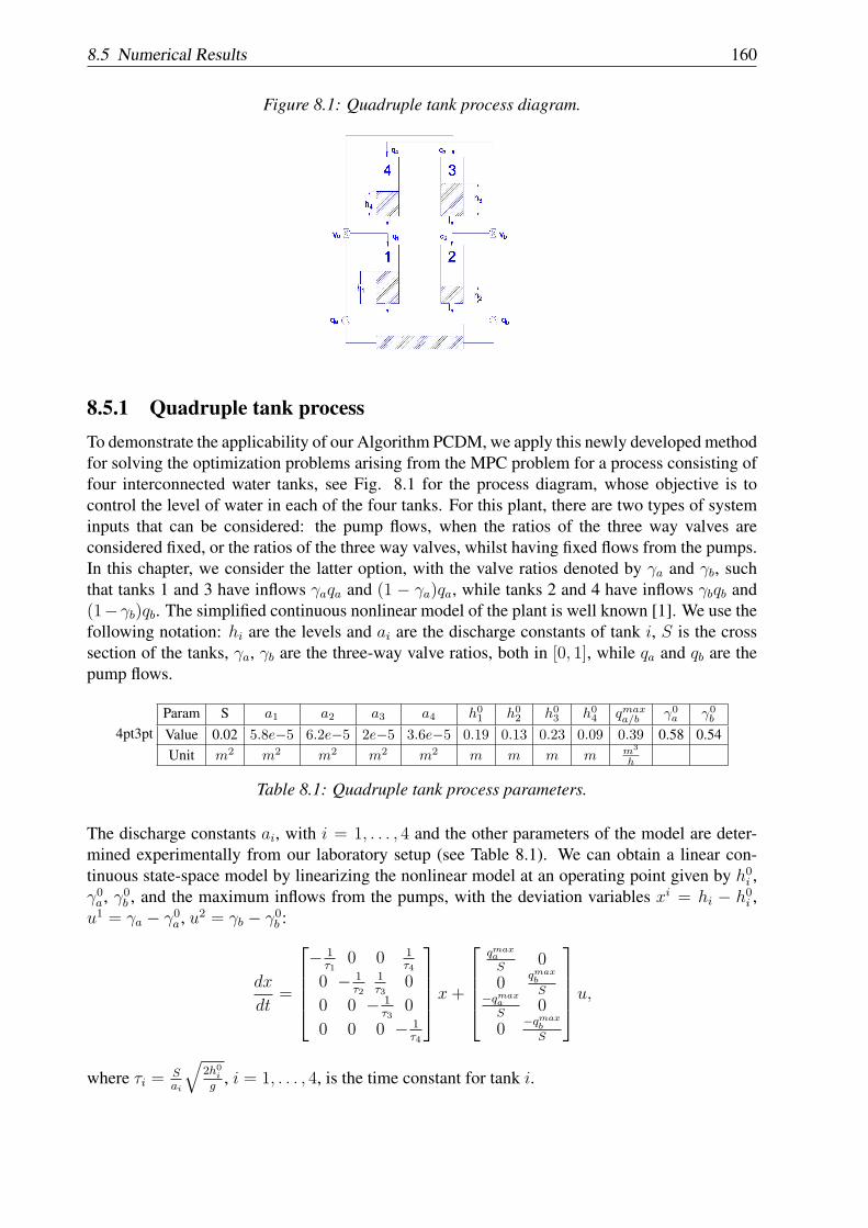
8.5 Numerical Results 160
Figure 8.1: Quadruple tank process diagram.
8.5.1 Quadruple tank processTo demonstrate the applicability of our Algorithm PCDM, we apply this newly developed methodfor solving the optimization problems arising from the MPC problem for a process consisting offour interconnected water tanks, see Fig. 8.1 for the process diagram, whose objective is tocontrol the level of water in each of the four tanks. For this plant, there are two types of systeminputs that can be considered: the pump flows, when the ratios of the three way valves areconsidered fixed, or the ratios of the three way valves, whilst having fixed flows from the pumps.In this chapter, we consider the latter option, with the valve ratios denoted by γa and γb, suchthat tanks 1 and 3 have inflows γaqa and (1 − γa)qa, while tanks 2 and 4 have inflows γbqb and(1−γb)qb. The simplified continuous nonlinear model of the plant is well known [1]. We use thefollowing notation: hi are the levels and ai are the discharge constants of tank i, S is the crosssection of the tanks, γa, γb are the three-way valve ratios, both in [0, 1], while qa and qb are thepump flows.
4pt3ptParam S a1 a2 a3 a4 h0
1 h02 h0
3 h04 qmax
a/b γ0a γ0
b
Value 0.02 5.8e−5 6.2e−5 2e−5 3.6e−5 0.19 0.13 0.23 0.09 0.39 0.58 0.54Unit m2 m2 m2 m2 m2 m m m m m3
h
Table 8.1: Quadruple tank process parameters.
The discharge constants ai, with i = 1, . . . , 4 and the other parameters of the model are deter-mined experimentally from our laboratory setup (see Table 8.1). We can obtain a linear con-tinuous state-space model by linearizing the nonlinear model at an operating point given by h0i ,γ0a, γ0b , and the maximum inflows from the pumps, with the deviation variables xi = hi − h0i ,u1 = γa − γ0a, u2 = γb − γ0b :
dx
dt=
− 1
τ10 0 1
τ4
0 − 1τ2
1τ3
0
0 0 − 1τ3
0
0 0 0 − 1τ4
x+
qmaxa
S0
0qmaxb
S−qmax
a
S0
0−qmax
b
S
u,
where τi = Sai
√2h0
i
g, i = 1, . . . , 4, is the time constant for tank i.

8.5 Numerical Results 161
Using zero-order hold method with a sampling time of 5 seconds we obtain the discrete timemodel of type (8.12), with the partition x1 ← [x1 x4]
T and x2 ← [x2 x3]T . For the input con-
straints of the MPC scheme we consider the practical constraints of the ratios of the three wayvalves for our plant, i.e ui ∈ [0.15, 0.8]− γi0, where γi0 is the linearization input. Due to the factthat our plant has overflow sensors fitted to the tanks and an emergency shutoff program, we donot introduce constraints for the states. For the stage cost we have taken the weighting matricesto be Qi = Ini
and Ri = 0.01Imi.
8.5.2 Implementation of the MPC scheme using MPIIn this section we underline the benefits of Algorithm PCDM when it is implemented in an ap-propriate fashion for the quadruple tank MPC scheme. We implemented for comparison, Algo-rithm PCDM and that of [103]. Both algorithms were implemented in C programming language,with parallelization ensured via MPI and linear algebra operations done with CLAPACK. Algo-rithm [103] requires solving, at each step, 2 QP problems in parallel, problems which cannotbe solved in closed form. For solving these QP problems, we use the qpip routine of the QPCtoolbox [118]. The algorithms were implemented on a PC, with 2 Intel Xeon E5310 CPUs at1.60 GHz and 4Gb of RAM. For the MPC problem in this subsection we control the plant suchthat the levels and inputs will reach those of the steady state linearization values h0 and γ0.
Figure 8.2: Total costs for 50 MPC steps with PCDM (white) and [103] (black).
0.2750
0.3500
0.5300
1150
275
350
530
τN
Figure 8.2 outlines a comparison of the two algorithms for solving this quadruple tank MPC prob-lem, considering a prediction time of 150 seconds, for different prediction horizons N and sam-
pling time τ , such that τN = 150 seconds. The bar values represent the total sum50∑t=1
VN(xt,u)
for 50 MPC steps, where u is calculated either with PCDM or with the algorithm from [103].For the same 50 simulation steps, we outline in Table 8.2 a comparison of the average number ofiterations achieved by both algorithms and the performance loss, i.e. a percentile difference be-
tween the suboptimal cost achieved in Figure 8.2 (50∑t=1
VN(xt,u)) and the optimal costs that were
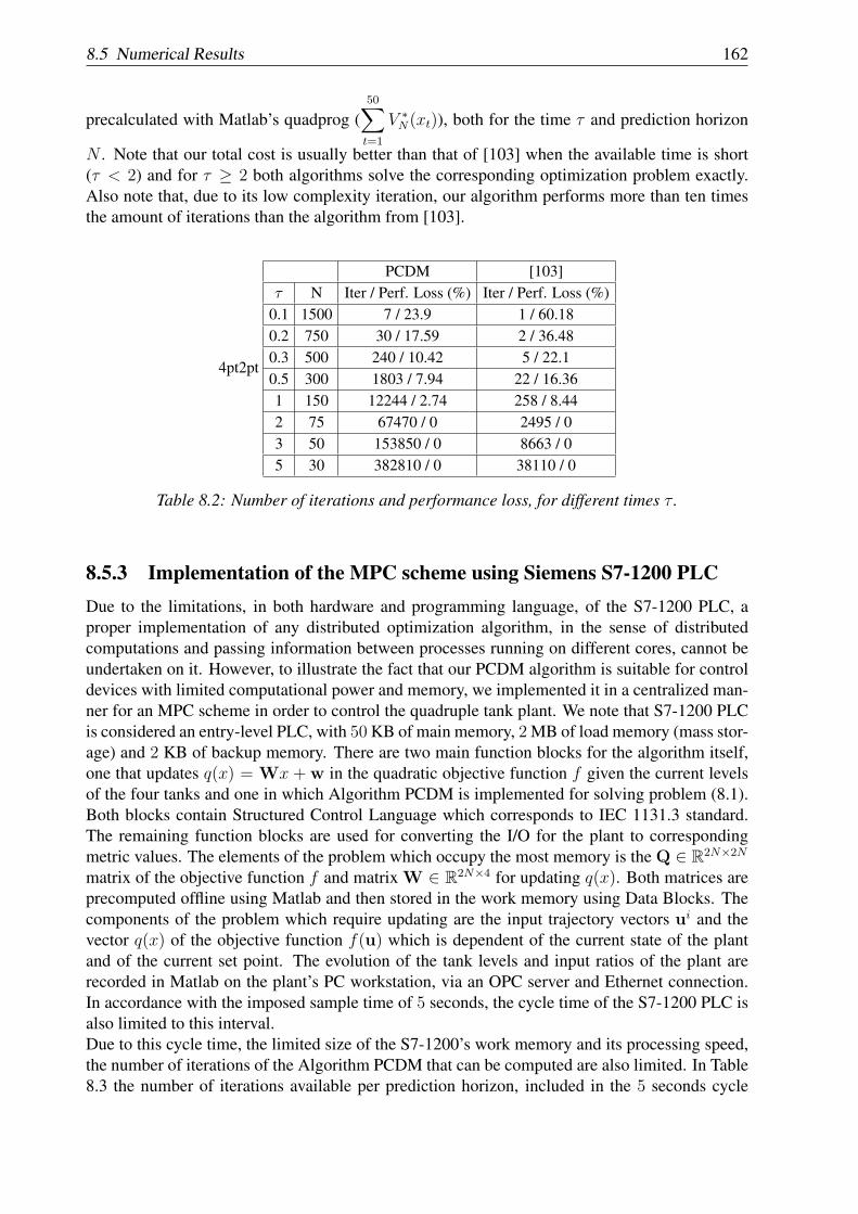
8.5 Numerical Results 162
precalculated with Matlab’s quadprog (50∑t=1
V ∗N(xt)), both for the time τ and prediction horizon
N . Note that our total cost is usually better than that of [103] when the available time is short(τ < 2) and for τ ≥ 2 both algorithms solve the corresponding optimization problem exactly.Also note that, due to its low complexity iteration, our algorithm performs more than ten timesthe amount of iterations than the algorithm from [103].
4pt2pt
PCDM [103]τ N Iter / Perf. Loss (%) Iter / Perf. Loss (%)
0.1 1500 7 / 23.9 1 / 60.180.2 750 30 / 17.59 2 / 36.480.3 500 240 / 10.42 5 / 22.10.5 300 1803 / 7.94 22 / 16.361 150 12244 / 2.74 258 / 8.442 75 67470 / 0 2495 / 03 50 153850 / 0 8663 / 05 30 382810 / 0 38110 / 0
Table 8.2: Number of iterations and performance loss, for different times τ .
8.5.3 Implementation of the MPC scheme using Siemens S7-1200 PLCDue to the limitations, in both hardware and programming language, of the S7-1200 PLC, aproper implementation of any distributed optimization algorithm, in the sense of distributedcomputations and passing information between processes running on different cores, cannot beundertaken on it. However, to illustrate the fact that our PCDM algorithm is suitable for controldevices with limited computational power and memory, we implemented it in a centralized man-ner for an MPC scheme in order to control the quadruple tank plant. We note that S7-1200 PLCis considered an entry-level PLC, with 50 KB of main memory, 2 MB of load memory (mass stor-age) and 2 KB of backup memory. There are two main function blocks for the algorithm itself,one that updates q(x) = Wx +w in the quadratic objective function f given the current levelsof the four tanks and one in which Algorithm PCDM is implemented for solving problem (8.1).Both blocks contain Structured Control Language which corresponds to IEC 1131.3 standard.The remaining function blocks are used for converting the I/O for the plant to correspondingmetric values. The elements of the problem which occupy the most memory is the Q ∈ R2N×2N
matrix of the objective function f and matrix W ∈ R2N×4 for updating q(x). Both matrices areprecomputed offline using Matlab and then stored in the work memory using Data Blocks. Thecomponents of the problem which require updating are the input trajectory vectors ui and thevector q(x) of the objective function f(u) which is dependent of the current state of the plantand of the current set point. The evolution of the tank levels and input ratios of the plant arerecorded in Matlab on the plant’s PC workstation, via an OPC server and Ethernet connection.In accordance with the imposed sample time of 5 seconds, the cycle time of the S7-1200 PLC isalso limited to this interval.Due to this cycle time, the limited size of the S7-1200’s work memory and its processing speed,the number of iterations of the Algorithm PCDM that can be computed are also limited. In Table8.3 the number of iterations available per prediction horizon, included in the 5 seconds cycle

8.5 Numerical Results 163
Cycle Time 5 sPrediction Horizon N 10 20 30Maximum Number of Iter. 104 39 15Used Memory (%) 59 72 88
Table 8.3: Available number of iterations and memory usage of Alg. PCDM
time, and the memory requirements for these prediction horizons are presented. Although thenumbers of computed iterations seem small, we have found in practice that the suboptimal MPCscheme still stabilizes the quadruple tank process and ensures set point tracking. The results of
Figure 8.3: Evolution of tank levels 1-4 (top), 2-3 (bottom), with continuous lines, against theirrespective set points, with dashed lines.
500 1000 1500 1800time(seconds)
h1sh1
h4sh4
500 1000 1500 1800time(seconds)
h2sh2
h3sh3
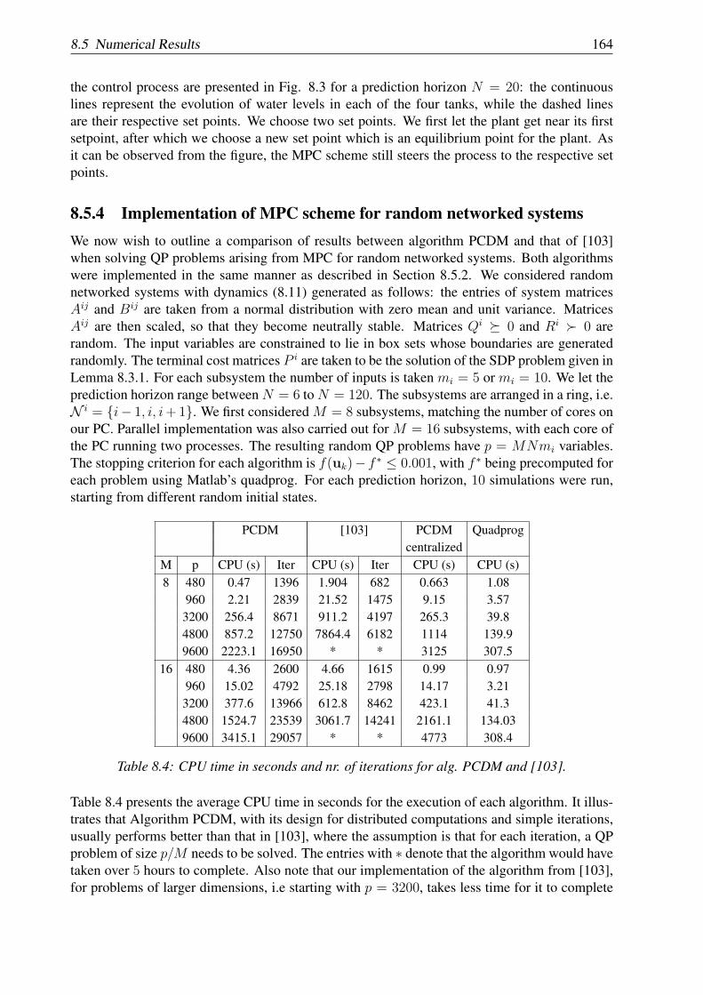
8.5 Numerical Results 164
the control process are presented in Fig. 8.3 for a prediction horizon N = 20: the continuouslines represent the evolution of water levels in each of the four tanks, while the dashed linesare their respective set points. We choose two set points. We first let the plant get near its firstsetpoint, after which we choose a new set point which is an equilibrium point for the plant. Asit can be observed from the figure, the MPC scheme still steers the process to the respective setpoints.
8.5.4 Implementation of MPC scheme for random networked systemsWe now wish to outline a comparison of results between algorithm PCDM and that of [103]when solving QP problems arising from MPC for random networked systems. Both algorithmswere implemented in the same manner as described in Section 8.5.2. We considered randomnetworked systems with dynamics (8.11) generated as follows: the entries of system matricesAij and Bij are taken from a normal distribution with zero mean and unit variance. MatricesAij are then scaled, so that they become neutrally stable. Matrices Qi ≽ 0 and Ri ≻ 0 arerandom. The input variables are constrained to lie in box sets whose boundaries are generatedrandomly. The terminal cost matrices P i are taken to be the solution of the SDP problem given inLemma 8.3.1. For each subsystem the number of inputs is taken mi = 5 or mi = 10. We let theprediction horizon range between N = 6 to N = 120. The subsystems are arranged in a ring, i.e.N i = i− 1, i, i+1. We first considered M = 8 subsystems, matching the number of cores onour PC. Parallel implementation was also carried out for M = 16 subsystems, with each core ofthe PC running two processes. The resulting random QP problems have p = MNmi variables.The stopping criterion for each algorithm is f(uk)− f ∗ ≤ 0.001, with f ∗ being precomputed foreach problem using Matlab’s quadprog. For each prediction horizon, 10 simulations were run,starting from different random initial states.
PCDM [103] PCDM Quadprogcentralized
M p CPU (s) Iter CPU (s) Iter CPU (s) CPU (s)8 480 0.47 1396 1.904 682 0.663 1.08
960 2.21 2839 21.52 1475 9.15 3.573200 256.4 8671 911.2 4197 265.3 39.84800 857.2 12750 7864.4 6182 1114 139.99600 2223.1 16950 * * 3125 307.5
16 480 4.36 2600 4.66 1615 0.99 0.97960 15.02 4792 25.18 2798 14.17 3.21
3200 377.6 13966 612.8 8462 423.1 41.34800 1524.7 23539 3061.7 14241 2161.1 134.039600 3415.1 29057 * * 4773 308.4
Table 8.4: CPU time in seconds and nr. of iterations for alg. PCDM and [103].
Table 8.4 presents the average CPU time in seconds for the execution of each algorithm. It illus-trates that Algorithm PCDM, with its design for distributed computations and simple iterations,usually performs better than that in [103], where the assumption is that for each iteration, a QPproblem of size p/M needs to be solved. The entries with ∗ denote that the algorithm would havetaken over 5 hours to complete. Also note that our implementation of the algorithm from [103],for problems of larger dimensions, i.e starting with p = 3200, takes less time for it to complete
8.5 Numerical Results 165
if the problem is divided between M = 16 subsystems than M = 8. This is due to the fact thatthe solver qpip takes much more time to solve problems of size 600 in the case of p = 4800 andM = 8 than problems of size 300 for p = 4800 and M = 16. Also, the transmission delays be-tween subsystems are negligible in comparison with these qpip times. We have also implementedAlgorithm PCDM in a centralized manner, i.e. without using MPI and, as can be seen from thetable, we gain speedups of computation when the algorithm is parallelized. Algorithm PCDMis outperformed by Matlab’s quadprog, but do note that quadprog is not designed for distributedimplementation and there are no transmission delays between processes.
Chapter 9
Future Work
Regarding the research directions that me, together with my group - “Distributed Control andOptimization (DCO)” group - we plan to pursue in the future spans along three fundamentalaxes:
(1) Huge-scale sparse optimization: theory, algorithms and applications
(2) Optimization based control for distributed networked systems
(3) Optimization based control for resource-constrained embedded systems
(1) The age of Big Data has begun. Data of huge sizes is becoming ubiquitous and prac-titioners in nearly all industries need to solve optimization problems of unprecedented sizes,but with specific structure, in particular sparsity. For example, in many applications from net-worked systems, distributed control, machine learning, compressed sensing, social networks andcomputational biology we can formulate sparse optimization problems with millions or billionsof variables. Classical first or second order optimization algorithms are not designed to scaleto instances of such huge sizes. As a consequence, new mathematical programming tools andmethods are required to solve efficiently these big data problems. For future research we plan todevelop new tools and optimization algorithms with low per-iteration cost and good scalabilityproperties for solving sparse huge scale optimization problems.
(2) & (3) From control point of view it is already recognized that mathematical optimizationand control are at the heart of the information and communication technologies of networked orembedded systems. Many control problems for complex networked systems can be formulated asoptimization problems but with sparse and structured matrix representations that can be exploitedin numerical optimization algorithms. Distributed optimization has been used for a long time indistributed estimation, distributed control or distributed model predictive control. Despite theprogress made in the last decades in this area, nearly all distributed schemes presented in theliterature suffer from slow convergence speeds, opening a window of opportunity for algorithmicresearch in this direction. Building on existing strengths on optimization algorithms of our group,we will concentrate on developing new efficient optimization schemes for complex systems.
Further, embedded systems interact with physical devices ranging from automotive enginesto mobile phones, robots and up to industrial installations. More than 90% of all CPUs are cur-rently deployed in embedded systems. Recently, a tremendous improvement of their performanceis noticeable for example in cars, where the increase of safety (ABS, ESP) and the reduction offuel consumption (EFI, EPS) were largely due to mechatronic design. The advances in sensortechnology, speed of processors and communication networks enable the use of embedded sys-tems with renewed functionalities and structures. The challenge in their integration is not the
166

9.1 Huge-scale sparse optimization: theory, algorithms and applications 167
lack of architecture flexibility or the available degrees of freedom but the complexity of controland supervision in itself. We plan to develop and overhaul the existing optimization-based con-trol techniques by implementation-oriented predictive controllers able to manage the embeddedsystems’ resources at the design stage.
9.1 Huge-scale sparse optimization: theory, algorithms andapplications
Many complexity results given by Nesterov (e.g. in [75]) provide a complete theory of optimiza-tion methods for general smooth/nonsmooth convex optimization problems. These results rep-resents a strong motivation to direct our future efforts for finding particular classes of structuredoptimization problems and consequently design appropriate first-order methods with computa-tional complexity guarantees for solving such problems. For example, it is known that for classesof optimization problems with objective functions satisfying an error bound property (which in-cludes the class of smooth strong convex objective functions) linear convergence can be provedfor certain type of descent methods [52,107]. Further, coordinate descent methods have recentlybecome very popular due to their low iteration cost and simplicity. We will further investigatethese issues through the following main research directions:
Research direction I: Structural analysis of specific classes of sparse huge scale optimizationproblems
i. Analysis of classes of optimization problems satisfying a global error bound property;
ii. Analysis of classes of optimization problems with sparsity-inducing penalties (e.g. lp-regularized problems, with 0 ≤ p ≤ 1);
iii. Dual formulations of separable optimization problems subject to intersection of a largenumber of convex sets.
Research direction II: Development of efficient numerical algorithms for problem classesanalyzed before
i Development and analysis of first-order methods for optimization problems satisfying aglobal error bound property;
ii. Development and analysis of first-order/coordinate descent methods for sparsity-regularized optimization problems;
iii. Analysis of primal-dual methods for solving optimization problems with separable struc-ture.
Research direction III: Implementation and benchmark of the developed numerical algo-rithms
i. Implementation of the algorithms in a toolbox;
ii. Benchmark the new developed algorithms on several engineering applications.
9.1 Huge-scale sparse optimization: theory, algorithms and applications 168
9.1.1 Methodology and capacity to generate resultsIt is remarkable how many current practical applications are formulated as sparse huge-scale op-timization problems : compressed sensing (find the most sparse solution of an underdeterminedlinear system), sensor network problem (reconstruct a signal from partial information), imagedeblurring or denoising (find the best approximation of a noisy image), controller synthesis (finda feedback gain law for controlling a system), support vector machine (find the best hyperplanewhich separates two classes of points), etc.Structural analysis of specific classes of sparse huge scale optimization problems: Globalerror bound property allows to obtain the linear convergence rate for certain gradient-based al-gorithms (e.g. descent type methods as proven in Chapter 7 or in papers [52, 107]). The classof functions satisfying the error bound property is much larger that the class of smooth stronglyconvex objective functions and arises naturally in many applications, e.g. the dual of a smoothconvex problem subject to linear constraints or certain quadratic problems. Recently, our group(see Chapter 7) but also Wang [116] have determined classes of convex smooth functions whichsatisfies globally the error bound property. However, there are still many open questions regard-ing this issue, e.g. determining whether a certain class of functions satisfies or not the globalerror bound property. Our goal is to investigate and describe general classes of optimizationproblems which satisfy the error bound property globally using tools from linear programmingand duality theory.
The interest in sparsity-regularized optimization problems and corresponding complexity is-sues has increased tremendously in the last decade, due to their application in many areas. Gen-erally, there are several results showing that one can obtain a sparse solution of an optimizationproblem by additively attaching to the objective function some specific regularizer. Typical reg-ularizers ensuring sparsity of the solution are the p-(quasi)norms (0 ≤ p ≤ 1). The main issue inregularizing the objective function with a quasinorm is the nonconvexity of the resulting prob-lem. For particular simple problems (e.g. quadratic problems), important properties for severalclasses of local minimizers have been established. However, no result of this kind is known forgeneral problems. This constitutes one of the issues that we aim to address, using tools fromconvex analysis which have been proven to be efficient in the case of l1-regularization.
Further, many practical engineering problems can be formulated as the minimization of asum of convex functions subject to a large intersection of convex sets. A lot of literature onthis subject generally develops “cheap” methods (e.g. incremental gradient methods) which useat each iteration partial first-order information of the objective function and partial informationof the feasible set. However, these methods are very slow and their analysis is conducted us-ing tools from nonsmooth optimization. Starting from standard duality theory, we will developtechniques for the reformulation of typical primal problems with the above-described structureinto easier dual problems. We will also quantify the structural difference and advantages of bothformulations.Development of efficient numerical algorithms for problem classes analyzed before: In re-cent years, gradient and coordinate descent methods have proven to be among the most success-ful approaches in big data optimization. Broadly speaking, gradient methods use only first orderinformation, while coordinate descent methods are based on the strategy of updating at each iter-ation a single block of coordinates of the vector of variables. Both approaches drastically reducethe memory requirements and arithmetic complexity of a single iteration.
An important issue for optimization problems satisfying an error bound property is to de-termine the classes of algorithms which attain linear convergence rate under this assumption.Until now, linear convergence has been established only for a particular class of gradient descent
9.1 Huge-scale sparse optimization: theory, algorithms and applications 169
methods (see e.g. Chapter 7 or papers [52, 107]). We will further investigate the class of fastgradient methods and other type of algorithms for which we can still achieve linear convergencerate. Starting from the results of [52, 107] given for descent-type methods, we will propose anextension to a more general class of algorithms, not necessarily of descent-type (e.g. acceleratedgradient method).
There has been an increasing interest in the last decade regarding the complexity of coordi-nate descent methods. However, many related issues still need to be solved. First, there existsno analysis of distributed or parallel coordinate descent strategies for composite convex opti-mization problems. Starting from our recent work presented in the previous chapters, we willprovide a complete complexity theory of distributed/parallel coordinate descent methods for gen-eral composite optimization problems. Second, there is no convergence analysis of coordinatedescent methods for general coupled constrained problems. Using the recent advances in thelinear case (see e.g. our previous chapters), we will develop further the theory for the generalcoupled constrained case.
Complexity results have recently been proposed for gradient methods applied for solvingl0-regularized optimization problems. We will extend the convergence analysis of these resultsto more efficient gradient-based algorithms (e.g. conditional gradient method, random coor-dinate descent method, accelerated gradient method), and analyze the performance of classicalfirst-order methods for l0-regularized optimization problems or more general sparsity-regularizedoptimization problems.Implementation and benchmark of the developed numerical algorithms: As practical effi-ciency is very important in all engineering areas, the efficient implementation and appropriatebenchmark of the developed algorithms are crucial in this project. For that reason, the ultimategoal of the project will consist in the production of a dedicated toolbox that will be able to solvespecific classes of sparse huge-scale optimization problems that cannot be solved with currentlyavailable software. The toolbox will be implemented in C code and Matlab code. Also, extensivecomparisons with state-of-the art algorithms and proper benchmarks of the developed algorithmswill be provided. Addressing these issues in an efficient fashion, we will bring sparse big dataoptimization one step closer to everyday use by practitioners, and we will enable its widespreaduse in real-world applications.
The convex optimization problem solver CVX, licensed by the Stanford group under thecoordination of Prof. Stephen Boyd, is increasingly popular. It is remarkable that the actualversion of CVX does not have any facilities for sparse large-scale optimization problems. Takinginto account the increasing number of applications of such type, our theoretical results couldserve as a foundation for a possible collaboration in the near future with the Stanford group, andultimately contribute to address the drawbacks of the CVX solver.
Effective radiation therapy, reduced computer tomography exposure and fast magnetic reso-nance imaging are just a few applications of sparse large-scale optimization theory in the clinicalmedicine area. Mathematical formulations of these problems share the same structural sparsity.Therefore, any advances and progress in the field of sparse optimization (as the objectives of thisproject claim) is mandatory for many aspects in the medical area. It is therefore a possibility todevelop future collaborations with partners from the medical field that do not possess a strongbackground in sparse large-scale optimization.
Compressed sensing, image deblurring/denoising, sparse classification and sparse clusteringare among the engineering problems which are formulated as distributed/centralized large-scalesparse optimization problems. As the main features of the toolbox (based on efficient solving ofsparse optimization problems) will ensure the entrance on the market and possible collaborationwith professionals from the signal processing and machine learning fields.
9.2 Optimization based control for distributed networked systems 170
9.2 Optimization based control for distributed networked sys-tems
Distributed optimization and control algorithms have to, in contrast to the centralized algorithms,satisfy an extra constraint, namely their computation shall be performed on separate units in par-allel, and the communication between these units is restricted. The communication constraintsmight come from judicial or game-theoretic restrictions, or from hardware constraints. The mainconcerns in the design of distributed algorithms are: the converge to a solution of the centralizedproblem and the rate of converge. The basic idea of decomposition is to decompose the originallarge problem into subproblems solved by independent units and then these units must negoti-ate their outcomes and requirements with their neighbors in order to achieve convergence to theglobal optimal solution. Distributed optimization methods already developed by our group takeadvantage of the sparsity and problem structure using parallel computations and duality theory.We will investigate further these directions of research:Research direction I: Distributed control based on decomposition optimization methods
i. developing new, efficient, robust, and scalable decomposition algorithms that shall offerfast convergence to the centrally optimal solutions;
ii. appropriately dealing with the computational complexity issues, problem structure, paral-lelism, various types of failures, and coordination and cooperation between the differentoptimization units;
iii. theoretical guarantees of stability and convergence speed under different initializations.
Research direction II: Design of sparse controllers for networked systems
i. developing structured controllers based on sparse optimization using lp regularized formu-lations;
iii. theoretical guarantees of stability and (sub)optimality of the controllers.
9.2.1 Methodology and capacity to generate resultsFor networked systems the optimization problem leads to sparse and structured matrix represen-tation, in particular block sparse or banded structures. The major difficulty for control is that dueto the enormous size of problems to be solved and communication restrictions, or requirementson robustness, often no central decisions can be taken, only local ones. Local decisions canpossibly be made with a (limited) view on the central objective in order to achieve faster conver-gence to overall system optimality. We will perform fundamental algorithmic research driven byapplications.
Distributed control based on decomposition optimization methods: The algorithm de-velopment will be based on the following principles: we will develop distributed algorithmsfor separable convex problems using the Lagrangian dual approach, accelerated schemes andsmoothing techniques in order to improve the convergence rates; we will also prove convergenceto the centrally optimal solution and the speed of convergence for the new methods; convex aswell as mildly non-convex models will be treated using Lagrangian dual approaches and accel-erated schemes; for mildly non-convex problems a scheme based on successive convex approxi-mations will be chosen; we will exploit the linear algebra structure of the problem, in particular
9.3 Optimization based control for resource-constrained embedded systems 171
block-sparse or banded structures; we will solve the local linear algebra problems in parallel andin an asynchronous computing environment. The research will result in systematic approachesthat outperform existing distributed control architectures and make distributed control a viablecontrol approach for controlling challenging large scale networked systems.
Design of sparse controllers for networked systems: We will design sparse and blocksparse feedback gains that are able to minimize a specific criterion associated to distributed sys-tems. Our approach will consists of two steps. Firstly, we will identify sparsity patterns offeedback gains by incorporating sparsity-promoting penalty functions into the optimal controlproblem, where the added terms penalize the number of communication links in the distributedcontroller (e.g. using lp regularizers). Secondly, we will optimize feedback gains subject to struc-tural constraints determined by the identified sparsity patterns using specialized optimizationalgorithms for solving this type of problems developed along first fundamental research focus.In particular, we take advantage of the separability of the sparsity-promoting penalty functionsto decompose the minimization problem into sub-problems that can be solved efficiently (evenanalytically). We will also investigate the tradeoff between the control requirements (guaran-tees of stability and (sub)optimality of the controllers) and sparsity requirements. In particular,we plan to propose methods able to alternate between promoting the sparsity of the controllerand optimizing the closed-loop performance and which allows us to exploit the structure of thecorresponding cost criterion.
9.3 Optimization based control for resource-constrained em-bedded systems
Another interesting research direction is the integration of the real-time constraints and com-puting limitations in the synthesis of optimization-based control laws. The goal is to handlethe truncation, finite representation, memory footprint or sampling rate limitation at the controldesign stage. As an example, the safe, comfortable and environmentally friendly functions ofa modern car (climate, brake or emission control) depend on about 100 embedded systems. Asignificant part of a new car’s development cost goes to the design of these systems’ software.More functionality is being realized via software rather than by dedicated mechanical compo-nents, leading to design flexibility and shorter time to market. We will further investigate theseissues through the following main research directions:Research direction I: Model predictive control under inexact numerical optimization: De-spite the progress made recently in this area, nearly all existing methods suffer from slow con-vergence speeds and complexity certification, opening a window of opportunity for algorith-mic research in this direction. Building on existing strengths on optimization algorithms of ourteam [64, 73], we will concentrate on developing new schemes with the following objectives:
i. development of new theoretical and numerical optimization control methods that are tai-lored to the real-time constraints and performance limitations of low cost embedded hard-ware;
ii. appropriately dealing with the computational complexity issues, problem structure, paral-lelism, effects of limited or variable precision arithmetic and various types of failures;
iii. provide theoretical guarantees of stability and convergence speed under different initializa-tions and demonstrate high-reliability of inexact numerical optimization control methods;
9.3 Optimization based control for resource-constrained embedded systems 172
iv. investigate the use of low cost hardware (e.g. FPGA) to accelerate the execution of numer-ical optimization algorithms for control through parallelism.
Research direction II: Stability and recursive feasibility certification in MPC: While someadvances have been made in guaranteeing stability and feasibility of suboptimal MPC schemes,this significant problem is still largely open. Recent advances led by our team [63, 66] haveshown that constraint tightening and set theoretic tools can be a viable alternative to these issues.The goal of this research is to extend these ideas to suboptimal solutions of more sophisticatedMPC schemes through:
i. development of efficient MPC schemes based on inexact numerical optimization algo-rithms and adaptive constraint tightening that will ensure feasibility and stability of thecontrol low generated by the algorithm;
ii. exploit the structure of the receding horizon optimization problems in the tailoring of thenumerical methods;
iii. development of an open platform incorporating advanced real-time optimization controlmethods for rapid deployment on real applications.
9.3.1 Methodology and capacity to generate resultsIn order to achieve these objectives, it is not possible to consider the behavior and performanceof optimization and control algorithms apart from the particular embedded systems hardwareon which they are implemented. Instead, it will be necessary to bring about a unification ofmethods from systems and control theory, mathematical optimization, mechanical and electronicengineering and computer science. We will generate theoretic results and concomitantly anchorthese developments to several classes of engineering applications with the ultimate goal of pro-ducing systematic tools for control design.From the theoretical point of view: The MPC law is based on the resolution of a finite opti-mization problem for a given regime (state and parameters). This optimization problem facesreal-time (finite resources and limited time) constraints and consequently we need to use inexactoptimization algorithms that have a priori bounds on the computational time. It is known how-ever that computation of bounds of this kind is usually not pursued in traditional optimization asreal-time setups are not common there. Starting from this constatation we will develop a body oftheoretical and numerical optimization control methods appropriate to the unique requirementsand limitations of low-cost embedded hardware. In particular we want to come up with conver-gence analysis for new gradient type methods [64, 73] (e.g. coordinate descent, conditional oraccelerated gradient), since usually this analysis can provide practical bounds while at the sametime being well suited for embedded implementations due to the simplicity of such methods.Another aspect will be the exploitation of structure in the problems that arise in control.
Another aspect will be the investigation of suboptimal MPC schemes which ensure feasibilityand stability with a limited number of optimization iterations. Since in many MPC schemesan approximate solution of the corresponding optimization problem might not be feasible, wepropose to solve approximately an auxiliary problem obtained by tightening the constraints ofthe original one [63, 66]. We will analyze the possibility of choosing adaptively the parametersmeasuring the suboptimality and tightening, since this will lead to a more flexible and potentiallyless conservative approach.From a practical and numerical point of view: Our aim is to apply the theoretical develop-ments above for a benchmark problem with the support of our partner Renault. From hardware
9.3 Optimization based control for resource-constrained embedded systems 173
perspective, there is the potential for customized number representations and massive parallelismboth due to the large matrix computations performed and due to the predictable nature of the dataflow, resulting in the opportunity for deep pipelining. However, the data-dependent nature of con-vergence detection poses new and exciting challenges for maximizing throughput given a flexiblecomputational architecture.
We will develop a platform containing different numerical algorithms and a set of routineswhich will allow to match an MPC problem with the appropriate optimization method. Thiswill automatize the time and hardware constraints, all by exploiting the structure of the controlproblem. For deployment of MPC laws, a set of routines will concentrate the systematic synthesisprocedure towards a specific architecture able to implement a certified implicit or alternativelyan explicit control law.
The advances in mathematical optimization will radically expand the scope of embeddedsystems to applications where unconventional models are available and tight bounds on resourcesare imposed. The resource-constrained algorithms the we plan to develop will be used in manyof existing embedded designs that can benefit from optimization. The proposed industrial casestudy will have a direct impact on automotive industry by demonstrating the practicality, easeand effectiveness of embedded control. Furthermore, the implementation of our results into atoolbox, where the selection and adjustment of the numerical routines are done autonomouslyand is aware of the particularities of the controlled process, will enable its widespread use inother real-time embedded applications.
The research group “Distributed Control and Optimization (DCO)” was established in 2010and at the moment is composed of Dr. Ion Necoara (head of the group) and three phd students:Drd. Valentin Nedelcu, Drd. Dragos Clipici and Drd Andrei Patrascu. Since 2012, Drd. DClipici was also hired as teaching assistant in our department. In conclusion, at the momentour group (DCO) has two permanent stuff members but we plan to further expand the group.In particular, in December 2013 Drd. V Nedelcu will defend his phd thesis and from February2014 we also plan to hire him as assistant professor in our department. In our group we have alsodeveloped several applications (a group of mobile robots e-puck but also a four tank installation).These applications allowed us to attract several bachelor and master student in interesting projectsassociated to these applications and we plan further to expand the range of practical applicationsavailable in our group.
Bibliography
[1] I. Alvarado, D. Limon, D. Munoz de la Pena, J.M. Maestre, M.A. Ridao, H. Scheu,W. Marquardt, R.R. Negenborn, B. De Schutter, F. Valencia, and J. Espinosa. A compar-ative analysis of distributed mpc techniques applied to the hd-mpc four-tank benchmark.Journal of Process Control, 21(5):800 –815, 2011.
[2] A. Auslender. Optimisation Methodes Numeriques. Masson, 1976.
[3] R.O. Barr and E.G. Gilbert. Some effcient algortihms for a class of abstract optimizationproblems arising in optimal control. IEEE Transaction on Automatic Control, 14:640–652,1969.
[4] H. Bauschke and J.M. Borwein. On projection algorithms for solving convex feasibilityproblems. SIAM Review, 38(3):367–426, 1996.
[5] A. Beck. The 2-coordinate descent method for solving double-sided simplex constrainedminimization problems. Technical report, Israel Institute of Technology, Haifa, Israel, dec2012.
[6] A. Beck and L. Tetruashvili. On the convergence of block coordinate descent type meth-ods. SIAM Journal on Optimization, 23(4):2037–2060, 2013.
[7] P. Berman, N. Kovoor, and P. M. Pardalos. Algorithms for least distance problem, Com-plexity in Numerical Optimization. World Scientific, 1993.
[8] D. P. Bertsekas. Nonlinear Programming, 2nd edition. Athena Scientific, Belmont, MA,1999.
[9] D.P. Bertsekas and J. Tsitsiklis. Paralel and Distributed Computation: Numerical Meth-ods. Prentice Hall, 1989.
[10] C.M. Bishop. Pattern Recognition and Machine Learning. Springer-Verlag, New York,2006.
[11] S. Bonettini. Inexact block coordinate descent methods with application to nonnegativematrix factorization. Journal of Numerical Analysis, 22:1431–1452, 2011.
[12] P.H. Calamai and J.J. More. Projected gradient methods for linearly constrained problems.Mathematical Programming, 39:93–116, 1987.
[13] E. Camponogara and H.F. Scherer. Distributed optimization for model predictive controlof linear dynamic networks with control-input and output constraints. IEEE Transactionson Automation Science and Engineering, 8(1):233–242, 2011.
174
Bibliography 175
[14] E. Candes, J. Romberg, and T. Tao. Robust uncertainty principles: Exact signal recon-struction from highly incomplete frequency information. IEEE Transactions on Informa-tion Theory, 52:489–509, 2006.
[15] A. Canutescu and R.L. Dunbrack. Cyclic coordinate descent: A robotics algorithm forprotein loop closure. Protein Science, 12:963–972, 2003.
[16] C. C. Chang and C. J. Lin. Libsvm: a library for support vector machines. ACM Transac-tions on Intelligent Systems and Technology, 27:1–27, 2011.
[17] K.W. Chang, C.J. Hsieh, and C.J. Lin. Coordinate descent method for large-scale l2-losslinear support vector machines. Journal of Machine Learning Research, 9:1369–1398,2008.
[18] O. Chapelle, V. Sindhwani, and S. Keerthi. Optimization techniques for semi-supervisedsupport vector machines. Journal of Machine Learning Research, 2:203–233, 2008.
[19] S. Chen, D. Donoho, and M. Saunders. Atomic decomposition by basis pursuit. SIAMReview, 43:129–159, 2001.
[20] X. Chen, M. K. Ng, and C. Zhang. Non-lipschitz ℓp -regularization and box constrainedmodel for image restoration. IEEE Transactions on Image Processing, 21(12):4709–4721,2012.
[21] P. L. Combettes. The convex feasibility problem in image recovery. In P. Hawkes, editor,Advances in Imaging and Electron Physics, pages 155–270. Academic Press, 1996.
[22] A.J. Connejo, R. Minguez, E. Castillo, and R. Garcia-Bertrand. Decomposition Tech-niques in Mathematical Programming: Engineering and Science Applications. Springer-Verlag, 2006.
[23] J.R. Correa, A.S. Schulz, and N.E. Stier Moses. Selfish routing in capacitated networks.Mathematics of Operations Research, pages 961–976, 2004.
[24] F. Deutsch and H. Hundal. The rate of convergence for the cyclic projections algorithm i:Angles between convex sets. Journal of Approximation Theory, 142:36–55, 2006.
[25] F. Deutsch and H. Hundal. The rate of convergence for the cyclic projections algorithm ii:Regularity of convex sets. Journal of Approximation Theory, 155:155–184, 2008.
[26] L. Fainshil and M. Margaliot. A maximum principle for positive bilinear control sys-tems with applications to positive linear switched systems. SIAM Journal of Control andOptimization, 50:2193–2215, 2012.
[27] M. Farina and R. Scattolini. Distributed predictive control: a non-cooperative algorithmwith neighbor-to-neighbor communication for linear systems. Automatica, 2012.
[28] C. Godsil and G. Royle. Algebraic graph theory. Springer, 2001.
[29] D. Goldfarb and S. Ma. Fast multiple splitting algorithms for convex optimization. Tech-nical report, Department of IEOR, Columbia University, 2010.
Bibliography 176
[30] L.G. Gubin, B.T. Polyak, and E.V. Raik. The method of projections for finding thecommon point of convex sets. Computational Mathematics and Mathematical Physics,7(6):1211–1228, 1967.
[31] G.M. Heal. Planning without prices. Review of Economic Studies, 36:347–362, 1969.
[32] Y.C. Ho, L.D. Servi, and R. Suri. A class of center-free resource allocation algorithms.Large Scale Systems, 1:51–62, 1980.
[33] B. Hu and A. Linnemann. Toward infinite-horizon optimality in nonlinear model predic-tive control. IEEE Transactions on Automatic Control, 47(4):679–682, 2002.
[34] L. Hurwicz. The design of mechanisms for resource allocation. American EconomicReview, 63:1–30, 1973.
[35] D. Hush, P. Kelly, C. Scovel, and I. Steinwart. Qp algorithms with guaranteed accuracyand run time for support vector machines. Journal of Machine Learning Research, 7:733–769, 2006.
[36] G.M. James, C. Paulson, and P. Rusmevichientong. The constrained lasso. Technicalreport, University of Southern California, 2013.
[37] J.L. Jerez, K.V. Ling, G.A. Constantinides, and E.C. Kerrigan. Model predictive con-trol for deeply pipelined field-programmable gate array implementation: algorithms andcircuitry. IET Control Theory and Applications, 6(8):1029–1041, 2012.
[38] A. Jokic and M. Lazar. On decentralized stabilization of discrete-time nonlinear systems.In Proceedings of American Control Conference, pages 5777–5782, 2009.
[39] J. Judice, M. Raydan, S. Rosa, and S. Santos. On the solution of the symmetric eigen-value complementarity problem by the spectral projected gradient algorithm. NumericalAlgorithms, 47:391–407, 2008.
[40] K. C. Kiwiel. On linear-time algorithms for the continuous quadratic knapsack problem.Journal of Optimization Theory and Applications, 134:549–554, 2007.
[41] D. Knuth. The art of computer programming. Addison-Wesley, Boston, USA, 1981.
[42] M. Kocvara and J. Outrata. Effective reformulations of the truss topology design problem.Optimization and Engineering, 2006.
[43] P. Komarek and A. Moore. Fast robust logistic regression for large sparse datasets withbinary outputs. In Artificial Intelligence and Statistics, 2003.
[44] N. Komodakis, N. Paragios, and G. Tziritas. Mrf energy minimization & beyond viadual decomposition. IEEE Transactions on Pattern Analysis and Machine Intelligence,33(3):531–552, 2011.
[45] J. Kurose and R. Simha. Microeconomic approach to optimal resource allocation in dis-tributed computer systems. IEEE Transactions on Computers, 38:705–717, 1989.
[46] D. Leventhal and A.S. Lewis. Randomized methods for linear constraints: Con-vergence rates and conditioning. Technical report, Cornell University, 2008.http://arxiv.org/abs/0806.3015.

Bibliography 177
[47] Y. Li and S. Osher. Coordinate descent optimization for l1 minimization with applicationto compressed sensing; a greedy algorithm. Inverse Problems and Imaging, 3:487–503,2009.
[48] D. Limon, T. Alamo, and E.F. Camacho. Stable constrained mpc without terminal con-straint. In Proceedings of American Control Conference, pages 4893–4898, 2003.
[49] C. J. Lin, S. Lucidi, L. Palagi, A. Risi, and M. Sciandrone. A decomposition algorithmmodel for singly linearly constrained problems subject to lower and upper bounds. Journalof Optimization Theory and Applications, 141:107–126, 2009.
[50] N. List and H. U. Simon. General polynomial time decomposition algorithms. LectureNotes in Computer Science, 3559:308–322, 2005.
[51] Z.Q. Luo and P. Tseng. Error bounds and convergence analysis of feasible descent meth-ods: A general approach. Annals of Operations Research, 46–47(1):157–178, 1993.
[52] Z.Q. Luo and P. Tseng. On the convergence rate of dual ascent methods for linearlyconstrained convex minimization. Mathematics of Operations Research, 18(2):846–867,1993.
[53] Z.Q. Luo and P. Tseng. A coordinate gradient descent method for nonsmooth separableminimization. Journal of Optimization Theory and Applications, 72(1), 2002.
[54] S. Ma and S. Zhang. An extragradient-based alternating direction method for convexminimization. Technical report, Chinese University of Hong Kong, January 2013.
[55] O.L. Mangasarian. Computable numerical bounds for lagrange multipliers of stationarypoints of non-convex differentiable non-linear programs. Operations Research Letters,4(2):47–48, 1985.
[56] M. Mongeau and M. Torki. Computing eigenelements of real symmetric matrices viaoptimization. Computational Optimization and Applications, 29:263–287, 2004.
[57] M.V. Nayakkankuppam. Solving large-scale semidefinite programs in parallel. Mathe-matical Programming, 109:477–504, 2007.
[58] I. Necoara. A random coordinate descent method for large-scale resource allocation prob-lems. In Proceedings of 51th IEEE Conference on Decision and Control, 2012.
[59] I. Necoara. Random coordinate descent algorithms for multi-agent convex optimizationover networks. IEEE Transactions on Automatic Control, 58(8):2001–2012, 2013.
[60] I. Necoara and D. Clipici. Distributed random coordinate descent methods for compositeoptimization. SIAM Journal of Optimization, partially accepted:1–41, 2013.
[61] I. Necoara and D. Clipici. Efficient parallel coordinate descent algorithm for convex opti-mization problems with separable constraints: application to distributed MPC. Journal ofProcess Control, 23(3):243–253, 2013.
[62] I. Necoara, D. Doan, and J. A. K. Suykens. Application of the proximal center decompo-sition method to distributed model predictive control. In Proceedings of the Conferenceon Decision and Control, pages 2900–2905, 2008.
Bibliography 178
[63] I. Necoara, L. Ferranti, and T. Keviczky. An adaptive constraint tightening approach tolinear mpc based on approximation algorithms for optimization. Optimal Control Appli-cations and Methods, in press:1–18, 2014.
[64] I. Necoara and V. Nedelcu. Rate analysis of inexact dual first order meth-ods: application to dual decomposition. IEEE Trans. Automatic Control, DOI:10.1109/TAC.2013.2294614:1–12, 2013.
[65] I. Necoara, V. Nedelcu, and I. Dumitrache. Parallel and distributed optimization methodsfor estimation and control in networks. Journal of Process Control, 21(5):756–766, 2011.
[66] I. Necoara, V. Nedelcu, T. Keviczky, M. D. Doan, and B. de Schutter. Stability of linearmodel predictive control based on tightening and approximate optimal control inputs. InProceedings of 52nd Conference on Decision and Control, 2013.
[67] I. Necoara, Y. Nesterov, and F. Glineur. A random coordinate descent method on largeoptimization problems with linear constraints. In Int. Conference on Continuous Opti-mization, 2013.
[68] I. Necoara, Y. Nesterov, and F. Glineur. A random coordinate descent method on large-scale optimization problems with linear constraints. Technical report, University Po-litehnica Bucharest, June 2013.
[69] I. Necoara and A. Patrascu. A random coordinate descent algorithm for singly linearconstrained smooth optimization. In Proceedings of 20th Mathematical Theory of Networkand Systems, 2012.
[70] I. Necoara and A. Patrascu. A random coordinate descent algorithm for optimization prob-lems with composite objective function and linear coupled constraints. ComputationalOptimization and Applications, DOI:10.1007/s10589-013-9598-8, 2013.
[71] I. Necoara and J.A.K. Suykens. Application of a smoothing technique to decomposition inconvex optimization. IEEE Transactions on Automatic Control, 53(11):2674–2679, 2008.
[72] I. Necoara and J.A.K. Suykens. An interior-point lagrangian decomposition method forseparable convex optimization. J. Optimization Theory and Applications, 143(3):567–588,2009.
[73] V. Nedelcu, I. Necoara, and D. Q. Quoc. Computational complexity of inexact gradientaugmented lagrangian methods: application to constrained mpc. SIAM Journal on Controland Optimization, 52(5):1–26, 2014.
[74] A. Nedic, A. Ozdaglar, and A.P. Parrilo. Constrained consensus and optimization in multi-agent networks. IEEE Transactions on Automatic Control, 55(4):922–938, 2010.
[75] Y. Nesterov. Introductory Lectures on Convex Optimization: A Basic Course. Kluwer,Boston, USA, 2004.
[76] Y. Nesterov. Efficiency of coordinate descent methods on huge-scale optimization prob-lems. SIAM Journal on Optimization, 22(2):341–362, 2012.
[77] Y. Nesterov. Subgradient methods for huge-scale optimization problems. CORE DIscus-sion Paper, 2012/02, 2012.
Bibliography 179
[78] Y. Nesterov. Gradient methods for minimizing composite objective functions. Mathemat-ical Programming, 140:125–161, 2013.
[79] Y. Nesterov. Gradient methods for minimizing composite objective functions. Mathemat-ical Programming, 140(1):125–161, 2013.
[80] Y. Nesterov and S. Shpirko. Primal-dual subgradient method for huge-scale lin-ear conic problems. Technical report, CORE, UCL, Louvain, Belgium, 2012.http://www.optimization-online.org/DB_FILE/2012/08/3590.pdf.
[81] F. Niu, B. Recht, C. Re, and S. Wright. Hogwild!: A lock-free approach to parallelizingstochastic gradient descent. NIPS, 2012.
[82] D.P. Palomar and M. Chiang. A tutorial on decomposition methods for network utilitymaximization. IEEE Journal on Selected Areas in Communications, 24(8):1439–1451,2006.
[83] B.N. Parlett. The Symmetric Eigenvalue Problem. SIAM, 1997.
[84] A. Patrascu and I. Necoara. Efficient random coordinate descent algorithms forlarge-scale structured nonconvex optimization. Journal of Global Optimization, DOI:10.1007/s10898-014-0151-9:1–31, 2013.
[85] A. Patrascu and I. Necoara. A random coordinate descent algorithm for large-scale sparsenonconvex optimization. In Proceedings of 12th European Control Conferencel, 2013.
[86] J. C. Platt. Fast training of support vector machines using sequential minimal optimization.Advances in Kernel Methods: Support Vector Learning, MIT Press, 1999.
[87] B.T. Poliak. Introduction to Optimization. Optimization Software, 1987.
[88] M.J.D. Powell. On search directions for minimization algorithms. Mathematical Pro-gramming, 4:193–201, 1973.
[89] Z. Qin, K. Scheinberg, and D. Goldfarb. Efficient block-coordinate descent algorithms forthe group lasso. Mathematical Programming Computation, 5(2):143–169, 2013.
[90] D.Q. Quoc, I. Necoara, and M. Diehl. Path-following gradient-based decompositionalgorithms for separable convex optimization. Journal of Global Optimization, DOI:10.1007/s10898-013-0085-7:1–25, 2013.
[91] D.Q. Quoc, I. Necoara, I. Savorgnan, and M. Diehl. An inexact perturbed path-followingmethod for lagrangian decomposition in large-scale separable convex optimization. SIAMJournal of Optimization, 23(1):95–125, 2013.
[92] J.B. Rawlings and D.Q. Mayne. Model Predictive Control: Theory and Design. Nob HillPublishing, 2009.
[93] P. Richtarik and M. Takac. Iteration complexity of randomized block-coordinate descentmethods for minimizing a composite function. Mathematical Programming, 2012.
[94] P. Richtarik and M. Takac. Parallel coordinate descent methods for big data optimization.Technical report, University of Edinburgh, Scotland, December 2012.
Bibliography 180
[95] S. M. Robinson. Bounds for error in the solution set of a perturbed linear program. LinearAlgebra and its Applications, 6:69–81, 1973.
[96] R.T. Rockafellar and R.J. Wets. Variational Analysis. Springer-Verlag, New York, 1998.
[97] R.T. Rockafeller. The elementary vectors of a subspace in rn. In Combinatorial Mathe-matics and its Applications, pages 104–127, Chapel Hill, North Carolina, 1969.
[98] R.T. Rockafeller. Network Flows and Monotropic Optimization. Wiley-Interscience, 1984.
[99] S. Ryali, K. Supekar, D. A. Abrams, and V. Menone. Sparse logistic regression for whole-brain classication of fmri data. NeuroImage, 51(2):752–764, 2010.
[100] S. Samar, S. Boyd, and D. Gorinevsky. Distributed estimation via dual decomposition. InProceedings European Control Conference (ECC), pages 1511–1516, 2007.
[101] H. Schwartz. Uber einen grenzubergang durch alternierendes verfahren. Vierteljahrss-chrift der Naturforschenden Gesselschaft in Zurich, 15:272–286, 1870.
[102] P.O.M. Scokaert, D.Q. Mayne, and J.B. Rawlings. Suboptimal model predictive control(feasibility implies stability). IEEE Transactions on Automatic Control, 44(3):648–654,1999.
[103] B. T. Stewart, A.N. Venkat, J.B. Rawlings, S. Wright, and G. Pannocchia. Cooperativedistributed model predictive control. Systems & Control Letters, 59:460–469, 2010.
[104] H.A.L. Thi, M. Moeini, T.P. Dihn, and J. Judice. A dc programming approach for solvingthe symmetric eigenvalue complementarity problem. Computational Optimization andApplications, 51:1097–1117, 2012.
[105] R. Tibshirani and J. Taylor. The solution path of the generalized lasso. Annals of Statistics,39(3):1335–1371, 2011.
[106] P. Tseng. Approximation accuracy, gradient methods and error bound for structured con-vex optimization. Mathematical Programming, 125(2):263–295, 2010.
[107] P. Tseng and S. Yun. A block-coordinate gradient descent method for linearly constrainednonsmooth separable optimization. Journal of Optimization Theory and Applications,140:513–535, 2009.
[108] P. Tseng and S. Yun. A coordinate gradient descent method for nonsmooth separableminimization. Mathematical Programming, 117(1–2):387–423, 2009.
[109] P. Tseng and S. Yun. A coordinate gradient descent method for linearly constrained smoothoptimization and support vector machine training. Computational Optimization and Ap-plications, 47:179–206, 2010.
[110] P. Tsiaflakis, I. Necoara, J. Suykens, and M. Moonen. Improved dual decompositionbased optimization for dsl dynamic spectrum management. IEEE Transactions on SignalProcessing, 58(4):2230–2245, 2010.
[111] V.N. Vapnik. The Nature of Statistical Learning Theory. Springer-Verlag, 1995.
Bibliography 181
[112] A.N Venkat, I.A. Hiskens, J.B Rawlings, and S. Wright. Distributed mpc strategies withapplication to power system automatic generation control. IEEE Transactions on ControlSystems Technology, 16(6):1192–1206, 2008.
[113] M. Vose. A linear algorithm for generating random numbers with a given distribution.IEEE Transactions on Software Engineering, 17(9):972–975, 1991.
[114] M. Wang and D. P. Bertsekas. Incremental constraint projection-proximal methods fornonsmooth convex optimization. Technical report, MIT, July 2013.
[115] P.W. Wang and C.J. Lin. Iteration complexity of feasible descent methods for convexoptimization. Technical report, National Taiwan University, 2013.
[116] P.W. Wang and C.J. Lin. Iteration complexity of feasible descent methods for convex opti-mization. Technical report, Department of Computer Science, National Taiwan University,2013.
[117] E. Wei, A. Ozdaglar, and A. Jadbabaie. A distributed newton method for network utilitymaximization. Technical Report 2832, Department of Electrical Engineering and Com-puter Science, Massachusetts Institute of Technology, 2011.
[118] A. Wills. QPC - Quadratic Programming in C. University of Newcastle, Australia, 2009.
[119] I.H. Witten, E. Frank, and M.A. Hall. Data Mining: Practical Machine Learning Toolsand Techniques. Elsevier, New York, 2011.
[120] S. Wright. Accelerated block coordinate relaxation for regularized optimization. Technicalreport, University of Wisconsin, 2010.
[121] L. Xiao and S. Boyd. Optimal scaling of a gradient method for distributed resource allo-cation. Journal of Optimization Theory and Applications, 129(3), 2006.
[122] S. Xu, M. Freund, and J. Sun. Solution methodologies for the smallest enclosing circleproblem. Computational Optimization and Applications, 25:283–292, 2003.
[123] G.X. Yuan, K.W. Chang, C.J. Hsieh, and C.J. Lin. A comparison of optimization meth-ods and software for large-scale l1-regularized linear classification. Journal of MachineLearning Research, 11:3183–3234, 2010.
[124] G.X. Yuan, C.H. Ho, and C.J. Lin. Recent advances of large-scale linear classification.Technical report, Department of Computer Science, National Taiwan University, 2011.
[125] S. Yun and K.C. Toh. A coordinate gradient descent method for l1-regularized convexminimization. Computational Optimization and Applications, 48:273–307, 2011.
[126] G. Zhao. A lagrangian dual method with self-concordant barriers for multistage stochasticconvex programming. Mathematical Programming, 102:1–24, 2005.