
SUMAR / CONTENTS 1/2009 - revistadestatistica.ro 01_2009.pdf · of some scientifi c paper works...
91
Romanian Statistical Review nr. 1 / 2009 SUMAR / CONTENTS 1/2009 REVISTA ROMÂNĂ DE STATISTICĂ www.revistadestatistica.ro O APLICAŢIE A METODELOR DE DETECTARE A VALORILOR ABERANTE PENTRU ÎMBUNĂTĂŢIREA CALITĂŢII INDICATORILOR ECONOMICI PE TERMEN SCURT 3 AN APPLICATION OF DATA EDITING METHODS TO IMPROVE DATA QUALITY OF SHORT-TERM BUSINESS STATISTICS 22 Dan Ion GHERGUŢ INSOMAR PIAŢA FORŢEI DE MUNCĂ DIN REGIUNEA SUD-EST 38 THE LABOR MARKET IN THE SOUTH- EAST REGION 46 Conf. univ. dr. Aurel Gabriel SIMIONESCU Conf. univ. dr. Marian CHIVU Universitatea “Constantin Brâncoveanu” Piteşti Drd. ec. Mirela CHIVU Agenţia pentru Dezvoltare Regională Sud-Est REZULTATE DISTRIBUŢIONALE ALE PROCESULUI POISSON- DIRICHLET DE DOUĂ VARIABILE 53 DISTRIBUTIONAL RESULTS OF THE TWO PARAMETER POISSON- DIRICHLET DISTRIBUTION 64 Lector univ. dr. Mihail BUŞU Universitatea „Spiru Haret” MANAGEMENTUL RISCURILOR ASOCIATE PROCESULUI DE IMPLEMENTARE A PROIECTELOR 74 THE MANAGEMENT OF THE RISKS ASSOCIATED WITH THE IMPLEMENTATION OF PROJECTS 79 Conf. univ. dr. Nicu MARCU Lect. univ. dr. Daniela GIURESCU Universitatea din Craiova EVENIMENT EDITORIAL LA SEMINARUL NAŢIONAL “OCTAV ONICESCU” 84
-
Upload
truongtuong -
Category
Documents
-
view
227 -
download
4
Transcript of SUMAR / CONTENTS 1/2009 - revistadestatistica.ro 01_2009.pdf · of some scientifi c paper works...

Romanian Statistical Review nr. 1 / 2009
SUMAR / CONTENTS 1/2009
REVISTA ROMÂNĂ DE STATISTICĂwww.revistadestatistica.ro
O APLICAŢIE A METODELOR DE DETECTARE A VALORILOR ABERANTE PENTRU ÎMBUNĂTĂŢIREA CALITĂŢII INDICATORILOR ECONOMICI PE TERMEN SCURT 3
AN APPLICATION OF DATA EDITING METHODS TO IMPROVE DATA QUALITY OF SHORT-TERM BUSINESS STATISTICS 22
Dan Ion GHERGUŢ INSOMAR
PIAŢA FORŢEI DE MUNCĂ DIN REGIUNEA SUD-EST 38 THE LABOR MARKET IN THE SOUTH- EAST REGION 46 Conf. univ. dr. Aurel Gabriel SIMIONESCU Conf. univ. dr. Marian CHIVU Universitatea “Constantin Brâncoveanu” Piteşti Drd. ec. Mirela CHIVU Agenţia pentru Dezvoltare Regională Sud-Est
REZULTATE DISTRIBUŢIONALE ALE PROCESULUI POISSON- DIRICHLET DE DOUĂ VARIABILE 53
DISTRIBUTIONAL RESULTS OF THE TWO PARAMETER POISSON- DIRICHLET DISTRIBUTION 64 Lector univ. dr. Mihail BUŞU
Universitatea „Spiru Haret”
MANAGEMENTUL RISCURILOR ASOCIATE PROCESULUI DE IMPLEMENTARE A PROIECTELOR 74 THE MANAGEMENT OF THE RISKS ASSOCIATED WITH THE IMPLEMENTATION OF PROJECTS 79
Conf. univ. dr. Nicu MARCU Lect. univ. dr. Daniela GIURESCU Universitatea din Craiova
EVENIMENT EDITORIAL LA SEMINARUL NAŢIONAL “OCTAV ONICESCU” 84
Romanian Statistical Review nr. 1 / 20092
Revista Română de Statistică, editată de Institutul Naţional de Statistică, este unica publicaţie de specialitate din ţara noastră în domeniul teoriei şi practicii statistice. Articolele publicate se adresează oamenilor de ştiinţă, cercetătorilor, precum şi utilizatorilor de date şi informaţii statistice interesaţi în lărgirea şi aprofundarea orizontului cunoaşterii prin asimilarea noţiunilor de specialitate, abordarea de noi lucrări şi studii de referinţă pe care să le aplice ulterior în domeniul în care îşi desfăşoară activitatea. Prin prezentarea unor lucrări ştiinţifi ce şi de promovare a culturii statistice, necesară în economia de piaţă funcţională, revista se doreşte a fi un spaţiu propice schimbului de idei şi, totodată, o provocare. Orice studiu sau opinie care poate contribui la dezvoltarea gradului de înţelegere a statisticii ca ştiinţă este binevenit.
The “Romanian Statistical Review”, published by the National Institute of Statistics is the only specialized statistical publication in Romania.The articles published apply to the scientists, researchers, and users of data and statistical information, interested in enlarging the knowledge horizon with specialty notions, new work papers and reference studies, to apply in their own fi eld. Through the presentation of some scientifi c paper works and statistical culture promotion, necessary for a functional market economy, the review wants to be a favorable space for debates and a challenge at the same time. Any study or opinion that can contribute to the development of the understanding degree of the statistics as a science is welcome.
La „Revue Statistique Roumaine”, editée par l’Institute National des Statistiques, est l’unique publication de spécialité de notre pays dans le domaine de la théorie et de la pratique statistique. Les articles publiés s’adressent aux scientifi ques, aux chercheurs, ainsi qu’aux utilisateurs de données et d’informations statistiques, interesés de développer leur horizon de conaissances avec des notions de spécialité, avec de nouveaux travaux et études de référence qu’on les applique ultériorement dans le domaine dans lequel ils déroulent leur activite. Par la présentation des certaines ouvrages scientifi ques et de promotion de la culture statistique, nécessaire dans l’économie de marché fonctionelle, la Revue se désire etre un espace propice pour l’échange des idées et en meme temps, une provocation. Chacune étude et opinion qui peut contribuer a la développement du degré de compréhension de la statistique comme science est bienvenue.
Revista Română de Statistică nr. 1 / 2009 3
O aplicaţie a metodelor de detectare a valorilor aberante pentru îmbunătăţirea calităţii indicatorilor economici pe termen scurt Dan Ion GHERGUŢ INSOMAR
Abstract Îmbunătăţirea calităţii datelor statistice este un obiectiv central al oricărui Institut Naţional de Statistică, eforturi majore fi ind dedicate furnizării de date corecte, relevante şi la timp către diversele categorii de utilizatori. Calitatea este, în cele din urmă, fundaţia credibilităţii statisticii ofi ciale. În procesul de producţie a indicatorilor economici pe termen scurt (Short Term Statistics – STS), specialiştii trebuie să judece cu atenţie echilibrul dintre calitate şi utilitate: datele de maximă acurateţe necesită mai mult timp şi mai multe resurse pentru producerea lor, însă interesul utilizatorilor se pierde în cazul când rezultatele sunt publicate prea târziu. Având în vedere cerinţele stricte ale statisticilor pe termen scurt, apare ca necesară punerea în practică a unor metode şi tehnici care să exploateze într-o cât mai mare măsură capacităţile tehnologiilor informatice, prin automatizarea proceselor de validare (curăţare) a datelor, în scopul reducerii timpului până la publicarea ofi cială a rezultatelor şi, în acelaşi timp, al păstrării calităţii pe întregul proces statistic. Articolul prezintă o procedură informatică SAS care operaţi-onalizează una din cele mai utilizate metode de identifi care automată a datelor aberante, cu aplicaţie în sfera anchetelor lunare în întreprinderi. Sunt prezentate, de asemenea, câteva consideraţii asupra unei metode utilizate în procesul de editare a datelor, absolut necesară pentru tratarea non-răspunsurilor parţiale prin tehnicile clasice de imputare – prin valori medii, hot-deck, date istorice şi, mai rar, prin imputare cold-deck – asigurând, în acelaşi timp, condiţiile de control aritmetic.
Statistică şi informatică
Romanian Statistical Review nr. 1 / 20094
Cuvinte cheie: STS, norme de editare a datelor/reguli de validare, standarde de calitate, SAS.
***
În Uniunea Europeană, producţia lunară a datelor statistice de intreprindere (aşa-numiţii indicatori economici pe termen scurt - STS) trebuie să fi e în conformitate cu dispoziţiile din Regulamentul Consiliului (CE) nr 1165/98, modifi cat de Regulamentul (CE) nr 1158 / 2005 a Parlamentului European şi a Consiliului. Regulamentul STS acoperă patru mari domenii: industrie, construcţii, comerţul cu amănuntul şi alte servicii, defi nite în conformitate cu clasifi carea NACE a activităţilor economice (NACE rev.2). Regulamentul STS indică şi variabilele, periodicitatea, nivelul de detaliu şi termenele limită pentru transmiterea rezultatelor la Eurostat. Termenele pot varia de la 15 zile până la 2 luni, în funcţie de tipul variabilei solicitate şi de grupul la care fi ecare stat membru aparţine, grupul fi ind defi nit de către contribuţia fi ecărei ţări la valoarea adăugată obţinută la nivelul UE. Cel mai adesea, presiunea de a avea date primare la un termen calendaristic rezonabil în fi ecare lună este direcţionată spre companii, care, uneori, trebuie să completeze chestionarele câteva zile înainte de încheirea rapoartelor fi nanciare. Direcţiile teritoriale de statistică şi echipele centrale încearcă să câştige un timp suplimentar pentru a colecta şi introduce datele, pentru a efectua validări preliminare, să încarce baza centrală de date şi apoi pentru a curăţa datele, să producă rezultate şi, în fi nal, să le difuzeze. Companiile au posibilitatea de a revizui datele lor anterior raportate cu ocazia următoarei anchete lunare, ceea ce implică în continuare faptul că toate datele trebuie să fi e în conformitate cu o serie de reguli de validare şi control1 cât mai precise şi cât mai cuprinzătoare posibil. Chiar dacă procedurile de introducere a datelor sunt proiectate să fi ltreze unităţile care au furnizat date eronate, unele inconsecvenţe ale datelor pot fi identifi cate doar când întregul set de date (fi şier) este disponibil, oferind posibilitatea de a explora datele istorice ale fi ecărei unităţi într-un anumit domeniu de analiză, dat de exemplu, prin activitatea lor economică şi clasa de mărime sau regiunea geografi că. Dorinţa de a difuza rezultatele cât mai curând posibil după fi nele lunii de referinţă oferă puţin timp pentru recontactarea companiilor sau pentru efectuarea de corecţii manuale, dacă sunt găsite erori. De fapt, faza de editare a datelor este una dintre cele mai mari consumatoare de timp după introducerea datelor brute şi, chiar dacă devine rutină, este crucială pentru calitatea rezultatelor. Este evident că procedurile de editare selectivă şi automată a datelor sunt necesare pentru a face faţă termenelor scurte standardelor de calitate. Înainte de aderarea României la Uniunea Europeană, Institutul
Statistică şi informatică
Revista Română de Statistică nr. 1 / 2009 5
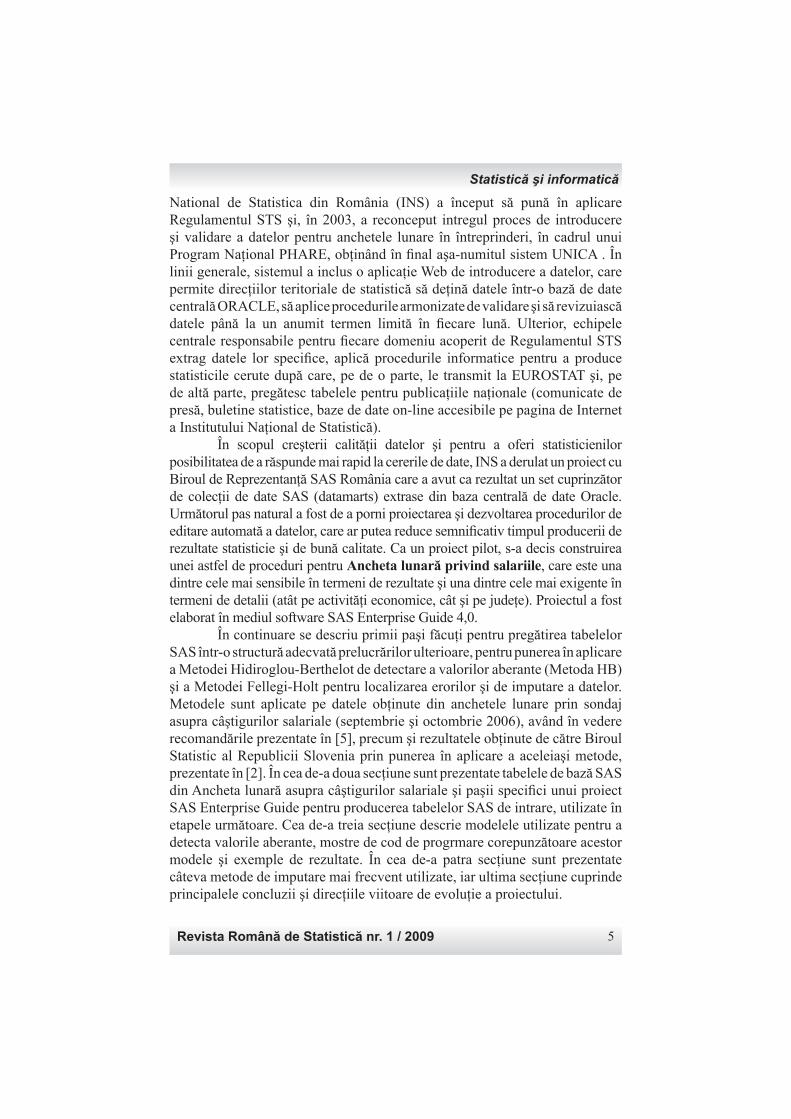
National de Statistica din România (INS) a început să pună în aplicare Regulamentul STS şi, în 2003, a reconceput intregul proces de introducere şi validare a datelor pentru anchetele lunare în întreprinderi, în cadrul unui Program Naţional PHARE, obţinând în fi nal aşa-numitul sistem UNICA . În linii generale, sistemul a inclus o aplicaţie Web de introducere a datelor, care permite direcţiilor teritoriale de statistică să deţină datele într-o bază de date centrală ORACLE, să aplice procedurile armonizate de validare şi să revizuiască datele până la un anumit termen limită în fi ecare lună. Ulterior, echipele centrale responsabile pentru fi ecare domeniu acoperit de Regulamentul STS extrag datele lor specifi ce, aplică procedurile informatice pentru a produce statisticile cerute după care, pe de o parte, le transmit la EUROSTAT şi, pe de altă parte, pregătesc tabelele pentru publicaţiile naţionale (comunicate de presă, buletine statistice, baze de date on-line accesibile pe pagina de Internet a Institutului Naţional de Statistică). În scopul creşterii calităţii datelor şi pentru a oferi statisticienilor posibilitatea de a răspunde mai rapid la cererile de date, INS a derulat un proiect cu Biroul de Reprezentanţă SAS România care a avut ca rezultat un set cuprinzător de colecţii de date SAS (datamarts) extrase din baza centrală de date Oracle. Următorul pas natural a fost de a porni proiectarea şi dezvoltarea procedurilor de editare automată a datelor, care ar putea reduce semnifi cativ timpul producerii de rezultate statisticie şi de bună calitate. Ca un proiect pilot, s-a decis construirea unei astfel de proceduri pentru Ancheta lunară privind salariile, care este una dintre cele mai sensibile în termeni de rezultate şi una dintre cele mai exigente în termeni de detalii (atât pe activităţi economice, cât şi pe judeţe). Proiectul a fost elaborat în mediul software SAS Enterprise Guide 4,0. În continuare se descriu primii paşi făcuţi pentru pregătirea tabelelor SAS într-o structură adecvată prelucrărilor ulterioare, pentru punerea în aplicare a Metodei Hidiroglou-Berthelot de detectare a valorilor aberante (Metoda HB) şi a Metodei Fellegi-Holt pentru localizarea erorilor şi de imputare a datelor. Metodele sunt aplicate pe datele obţinute din anchetele lunare prin sondaj asupra câştigurilor salariale (septembrie şi octombrie 2006), având în vedere recomandările prezentate în [5], precum şi rezultatele obţinute de către Biroul Statistic al Republicii Slovenia prin punerea în aplicare a aceleiaşi metode, prezentate în [2]. În cea de-a doua secţiune sunt prezentate tabelele de bază SAS din Ancheta lunară asupra câştigurilor salariale şi paşii specifi ci unui proiect SAS Enterprise Guide pentru producerea tabelelor SAS de intrare, utilizate în etapele următoare. Cea de-a treia secţiune descrie modelele utilizate pentru a detecta valorile aberante, mostre de cod de progrmare corepunzătoare acestor modele şi exemple de rezultate. În cea de-a patra secţiune sunt prezentate câteva metode de imputare mai frecvent utilizate, iar ultima secţiune cuprinde principalele concluzii şi direcţiile viitoare de evoluţie a proiectului.
Statistică şi informatică
Romanian Statistical Review nr. 1 / 20096
Descrierea tabelelor SAS primare şi pregătirea tabelelor SAS de intrare
Structura tabelelor SAS primare ale Anchetei lunare asupra câştigurilor salariale corespund principiilor aplicaţiilor de introducere a datelor utilizate în INS pentru toate anchetele statistice: fi ecare chestionar sau formular statistic este văzut ca o combinaţie de “capitole”, iar în fi ecare “capitol” există un set de rânduri şi de coloane. În cazul anchetei sunt două “capitole”. Primul capitol conţine ca rânduri variabilele statistice despre salarii şi câştiguri (într-un numar de 12) şi cel de-al doilea capitol conţine rânduri privind numărul de persoane angajate şi orele lucrate (într-un număr de 8). Drept coloane, tabela SAS include date cu privire la principalele activităţi economice şi secundare desfăşurate de companie. Fiecare înregistrare reprezintă o combinaţie de rânduri şi coloane. Dacă solicităm date despre salariile brute plătite, iar compania, pe lângă activitatea principală, are două alte activităţi secundare, va exista un rând (înregistrare) pentru salariile brute plătite aferente activităţii economice principale şi alte două rânduri, pentru fi ecare activitate secundară identifi cată. În realitate, fi ecare companie are şi un rând care este totalul rândurilor următoare ale respectivei companii. Chiar dacă acest rând reprezintă o povară suplimentară pentru companie, el este considerat ca o cheie de control importantă atât pentru companie, cât şi pentru ofi ciul de statistică. În scopul identifi cării unităţii de tip de activitate (KAU2) pentru toate companiile observate, chestionarul este conceput pentru a colecta date privind activitatea principală şi un număr de maxim 13 activităţi secundare exercitate. Numărul de activităţi secundare a fost derivat din experienţa anchetelor anterioare lunare şi anuale în întreprinderi. Astfel, pentru aproximativ 20.000 de companii incluse în ancheta lunară, tabela SAS primară are aproximativ 5.500.000 de rânduri. Fiecare înregistrare a unei unităţi conţine toate celulele determinate de rânduri şi de coloane, indiferent cât de multe activităţi are: 1 sau alte 13. Principalele variabile ale tabelei SAS primare pentru fi ecare lună sunt: luna anchetei, identifi catorul unităţii, identifi carea celulei din chestionar (cu indicarea corespunzătoare a rândului şi a coloanei), clasa NACE şi valoarea celulei. Doar un număr limitat de companii au mai multe activităţi secundare şi cea mai mare parte a celulelor sunt completate cu zero. După recodifi carea valorilor NACE - întrucât în tabela SAS primară, valoarea NACE pentru totaluri a fost marcată cu valoare lipsă (missing) - şi a denumirii variabilelor, în scopul folosirii lor în următoarele proceduri ca vectori, tabelele SAS au fost transpozate pentru a construi rânduri separate pe fi ecare companie pentru totaluri, activitate principală şi activităţile secundare existente, împreună cu un set unic de 20 de variabile de observare. Acest tip de structură a fost preferat faţă de o altă posibilă soluţie, respectiv, să aibă un rând unic pentru fi ecare companie, iar drept coloane să conţină un set de
Statistică şi informatică
Revista Română de Statistică nr. 1 / 2009 7
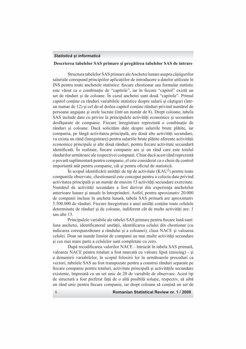
20 de variabile de observare, înmulţit cu 14 activităţi (o activitate principală şi 13 secundare), indiferent de numărul de activităţi secundare exercitate în realitate de companie şi, implicit, raportate pentru luna observată. Structura pentru care s-a optat este utilă pentru construirea separată de agregări pe activităţi economice, fi e prin luarea în considerare a activităţii principale, fi e a activităţilor omogene (principală sau secundară).Un exemplu al conţinutului tabelei SAS, după transpozare, este prezentat în continuare.
Conţinutul tabelei SAS pentru Ancheta lunară privind câştigurile salariale (fragment)
Tabelul 1Identifi -
cator (ID)
CAENprincipal
CAEN R01 … R08 … R13 … R18 R19 R20
2361542 1822 0 19882 … 20539 … 52 … 8736 0 0
2361542 1822 1822 19882 … 20539 … 52 … 8736 0 0
2768181 9131 0 75704 … 75704 … 65 … 15973 0 0
2768181 9131 9131 75704 … 75704 … 65 … 15973 0 0
2770487 5050 0 55554 … 56439 … 104 … 10720 0 0
2770487 5050 5050 34828 … 34828 … 104 … 5464 0 0
2770487 5050 5212 7629 … 7629 … 78 … 2080 0 0
2770487 5050 5530 6781 … 7228 … 40 … 1784 0 0
2770487 5050 6024 6316 … 6754 … 14 … 1392 0 0
2770499 5211 0 65125 … 66109 … 13 … 13104 0 0
2770499 5211 5211 53755 … 54739 … 11 … 10584 0 0
2770499 5211 5139 2750 … 2750 … 78 … 504 0 0
2770499 5211 1581 6438 … 6438 … 63 … 1512 0 0
2770499 5211 5530 2182 … 2182 … 3 … 504 0 0
În coloana CAEN, codul “0” semnifi că rândul de total, ca o sumă a valorilor raportate pentru activităţile principale şi secundare, dacă este cazul. Primele două companii (ID=2361542 şi ID=2768181) au raportat doar o activitate (principală) şi fi ecare dintre ultimele două (ID=2770487 şi ID=2770499) au raportat alte trei activităţi secundare, în plus faţă de cea principală. Acest simplu “truc” de codifi care a activităţii CAEN cu 0 permite agregarea cifrelor totale pe activitatea CAEN principală (excluzând alte rânduri) sau la agregare de activităţi omogene, adică pe “CAEN”, excluzând rândurile de total. Pentru a oferi o imagine asupra conţinutului variabilelor, variabila R01 înseamnă suma totală a salariilor brute plătite din fondul de salarii, R08 este suma totală a plăţilor brute (inclusiv bonusuri, prime, plăţi pentru
Statistică şi informatică
Romanian Statistical Review nr. 1 / 20098
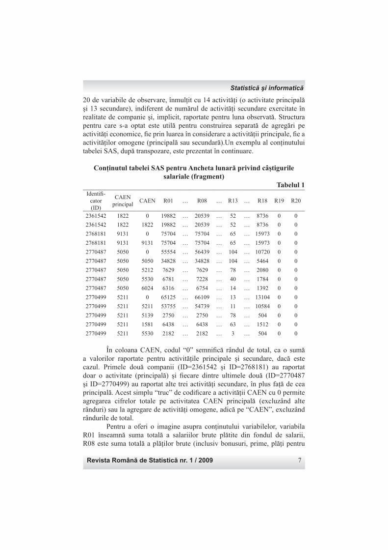
concedii de boală etc. ), R13 este numărul total de salariaţi la sfârşitul lunii, R18 şi R19 arată numărul total de ore lucrate în programul normal de timp şi ore suplimentare şi R20 numărul total de salariaţi care nu se afl ă pe statul de salarizare sau nu au un contract (exemplu, angajatori sau membri de familie). Pentru tabela fi nală SAS a lunii este necesar un număr de variabile suplimentare: cod de non-răspuns, care ajută la identifi carea unităţilor care nu au raport din mai multe motive (refuz, inchise temporar, fără activitate etc.) şi ponderile de sondaj. Aceste variabile sunt adăugate la fi şierul din tabele SAS separate.
Diagrama fl uxului de proces “Prepare Data” - Proiect ESOPFigura 1
Recodificare câmpuri cod CAEN "i câmpuri
date
Citire tabele primare SAS
pentru luna n-1 "i n
Tranpozare tabel SAS (normalizare structur )
Redresare e"antion (recalculare coeficien!i
extindere)
Concatenare tabele SAS luna n-1 "i n
Descrierea Metodei Hidiroglou-Berthelot
Procesul de editare are două faze majore. În timpul primei faze, care este pusă în aplicare în procesul de introducere a datelor, sunt testate principalele condiţii de control, în termeni de coerenţă a relaţiilor dintre variabile la nivel micro. Orice eroare (din cele programate) este semnalată şi responsabilul direcţiei teritoriale de statistică reverifi că datele din chestionar şi, dacă este necesar, contactează din nou compania pentru mai multe clarifi cări. De asemenea, sunt produse tabele de erori, indicând compania şi tipul de eroare care a avut loc. Această etapă necesită mult timp, iar în majoritatea cazurilor datele raportate sunt confi rmate.
Statistică şi informatică
Revista Română de Statistică nr. 1 / 2009 9
În cea de-a doua fază, la nivel central, o procedură de validare execută acelaşi tip de controale pentru a identifi ca orice înregistrări eronate, care ar fi putut fi ignorate de către direcţiile teritoriale de statistică. În acelaşi timp, datele raportate pentru luna curentă sunt verifi cate faţă de luna anterioară sau cu un istoric al datele raportate în timpul ultimului an. Doar dacă apar diferenţe mari, de echipa de anchetă centrale responsabile solicită din nou direcţia teritorială pentru a verifi ca dacă datele raportate sunt corecte sau nu. Cea mai mare parte a datelor este confi rmată, astfel încât nu este operată nici o corecţie. În această abordare clasică, volatilitatea unor variabile poate infl uenţa mult extinderea fi nală, deoarece cercetarea statistică este prin sondaj. Modifi cările de la o lună la alta, chiar dacă sunt confi rmate de către companie, nu pot fi atribuite tuturor companiilor care sunt reprezentate de unitatea din eşantion. În scopul diminuării infl uenţei modifi cărilor observate, este necesară a treia fază, care constă în combinarea editării automate cu cea selectivă şi cu imputarea automată, ţinând cont de comportamentul tuturor unităţilor respondente care sunt similare cu acele unităţi detectate cu variabile ale căror valori sunt aberante. Aplicate în cazul nostru, poate este necesară menţionarea unui detaliu: detectarea valorilor aberante ia în considerare numai acele companii care au răspuns în ambele anchete lunare. Cele care au răspuns numai pentru o perioadă sunt excluse din tabela SAS de detectare a valorilor aberante. Identifi carea valorilor aberante se bazează pe Metoda HB, care utilizează raportul dintre valorile observate ale variabilelor în două perioade consecutive de timp (luni, în cazul nostru). Modelul necesită defi nirea domeniilor de analiză, şi anume, grupuri de companii în care se realizează detectarea valorilor aberante. Aceste domenii pot fi construite din activităţi economice (secţiune/diviziune/grupă CAEN) şi clase de mărime, în funcţie de numărul mediu de persoane angajate de către fi ecare companie în luna observată. Raţiunea construirii domeniului de analiză este acela de a pune împreună unităţi similare, al căror comportament este cât se poate de omogen. Pe parcursul implementării modelului, una din opţiuni a fost de a construi domenii pe grupe CAEN, mai exact primele trei cifre ale clasei CAEN, combinat cu clase de mărime. Rezultatul a fost o fragmentare destul de ridicată, obţinând domenii cu un număr foarte redus de respondenţi, chiar domenii cu o singură companie. În aceste domenii mici, modelul are tendinţa de a semnala valori aberante indiferent de cât de bune sau rele par să fi e cifrele de la o perioadă la alta. Cea de-a doua opţiune a fost de a diviza domeniile pe diviziuni CAEN (de exemplu, primele două cifre ale clasei CAEN), care ar putea fi recomandată. Desigur, decizia fi nală ar trebui să fi e luată de către analist.
Statistică şi informatică
Romanian Statistical Review nr. 1 / 200910
Notaţii necesare pentru descrierea modelului: Pentru orice unitate i, avem 20 variabile yijt, unde j este indicele variabilei (j = 1 ÷ 20) şi t desemnează cele două perioade de timp (t = 1 şi t = 2). Raportul dintre cele două variabile desemnate de perioada de timp se numeşte trend:
>
=
altfel
yisexistaydacay
y
t jijiji
ji
ji
,0
0 , 1, 1, 1,
2,
(1)
În cadrul fi ecărui domeniu, se calculează Mediana neponderată a acestor trenduri: djtmed )( , unde d este domeniul. Utilizând mediana trendurilor, pentru fi ecare unitate se calculează un scor, desemnat să asigure simetria cozilor distribuţiei trendurilor:
≥−
≤<−=
djjidjji
djjijidj
ji tmedtfitmedt
tmedtfittmeds
)( ,1)(/
)(0 ,/)(1
(2)
Dacă tij este zero, scorul corespunzător nu este defi nit, ceea ce ar trebui să conducă la marcarea implicită a acestei înregistrări ca valoare aberantă. Este fi resc ca scorul să nu fi e defi nit, dacă pentru luna precedentă unitatea a raportat o valoare diferită de zero pentru o anumită variabilă şi egală cu zero pentru luna următoare sau vice-versa. În realitate, această situaţie ar putea apărea, de exemplu, în cazul concediilor medicale sau al plăţii de bonusuri. Se procedează la a doua transformare, pentru a combina scorul cu magnitudinea datei de analizat, rezultând efectul:
1] ),( [max 2, 1, c
jijijiji yysE = (3)
unde c1 este un parametru de reglaj cu valori între 0 şi 1. Dacă c1 este setat la zero, efectul este echivalent cu sij, omiţând să ia în considerare dimensiunea unităţii. Dacă este setat la 1, cu cât este mai mare valoarea variabilei, cu atât va infl uenţa mai mult determinarea valorii aberante. În literatura de specialitate, parametrul c1 este setat la 0,5. Se calculează scala din stânga şi dreapta cozii distribuţiei efectelor. Se calculează cuartilele efectelor în cadrul fi ecărui domeniu particular pentru toate variabilele: EQ1, EQ2 şi EQ3.. Scala din stânga şi dreapta cozilor sunt defi nite prin: ],max[ 2212, QQQleftj EcEEd −= (4)
],max[ 2223, QQQrightj EcEEd −= (5)
Statistică şi informatică
Revista Română de Statistică nr. 1 / 2009 11
Cea de-a doua parte a funcţiei de maximizare oferă posibilitatea de a preveni căutarea datei corecte în regiunile afl ate prea aproape de medie. În practică, parametrul de ajustare c2 este setat la 0,05. În cazul în care efectele sunt în afara intervalului ],[ ,32,32 rightjQleftjQ dcEdcE ⋅+⋅− (6) valoarea variabilei corespunzătoare este marcată ca valoare aberantă. Parametrul c3 determină lărgimea intervalului de acceptare, cu un maxim de 100. În literatura de specialitate, valoarea recomandată este de 40. Cu cât parametrul este setat la valori mai mari, zona de respingere devine mai mică, iar marcajul de valoare aberantă indică unităţi şi variabile ce trebuie verifi cate. A fost testat un set de trei valori ale parametrului c3, ca urmare a abordării sugerate în [3]: 20, 40 şi 50. Folosind o valoare de 20, metoda a indicat 6370 de unităţi având una sau mai multe variabile marcate ca valori aberante, 6013 pentru o valoare de 40 şi 5943 de unităţi pentru o valoare de 50. Valorile aberante declarate pentru c3 = 50 sunt, în general, suprimate din baza de imputare şi de revizuire a analistului, desemnându-le pentru imputare automată. În cazul nostru, încă mai există valori aberante implicite marcate datorită valorilor zero pentru luna curentă, sau, în domeniile de analiză de dimensiui reduse, din cauza unor mici schimbări de la o lună la alta. Indiferent de valoarea parametrului ales, este recomandat ca analistul să verifi ce valorile aberante şi să anuleze marcajul, dacă se consideră că valoarea raportată ca fi ind exactă, începând cu setul de date stabilit de către cea mai mare valoare a parametrului c3. Faţă de metoda de detectare a valorilor aberante bazată pe calculul efectelor, o altă soluţie este de a defi ni limite pentru fi ecare variabilă şi pentru fi ecare unitate. În acest scop, o metodă este sugerată în [4], constând în transformările inverse. Limitele inferioare şi superioare ale scorurilor se calculează utilizând următoarele formule:
( ) 1 ),max( 2, 1,
,32, c
jiji
leftjQdl yy
dcEs
⋅−= (7)
( ) 1 ),max( 2, 1,
,32, c
jiji
rightjQdu yy
dcEs
⋅+= (8)
Limitele inferioare şi superioare ale Medianei trendurilor sunt:
)1()(
,l
djdl s
tmedt −= (9)
)1()(, udjdu stmedt +⋅=
(10)
Statistică şi informatică
Romanian Statistical Review nr. 1 / 200912
Limitele inferioare şi superioare ale fi ecărei valori ale variabilei sunt date de:
1, ,, jidldl yty ⋅= (11)
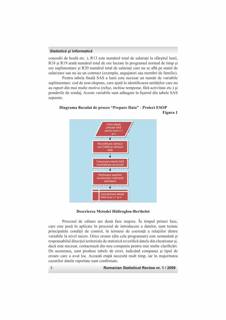
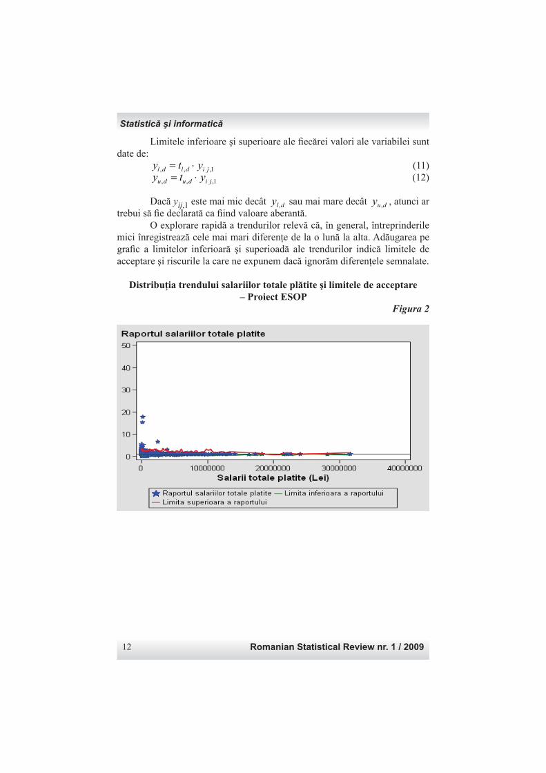
1, ,, jidudu yty ⋅= (12) Dacă yij,1 este mai mic decât dly , sau mai mare decât duy , , atunci ar trebui să fi e declarată ca fi ind valoare aberantă. O explorare rapidă a trendurilor relevă că, în general, întreprinderile mici înregistrează cele mai mari diferenţe de la o lună la alta. Adăugarea pe grafi c a limitelor inferioară şi superioadă ale trendurilor indică limitele de acceptare şi riscurile la care ne expunem dacă ignorăm diferenţele semnalate.
Distribuţia trendului salariilor totale plătite şi limitele de acceptare – Proiect ESOP
Figura 2
Statistică şi informatică
Revista Română de Statistică nr. 1 / 2009 13
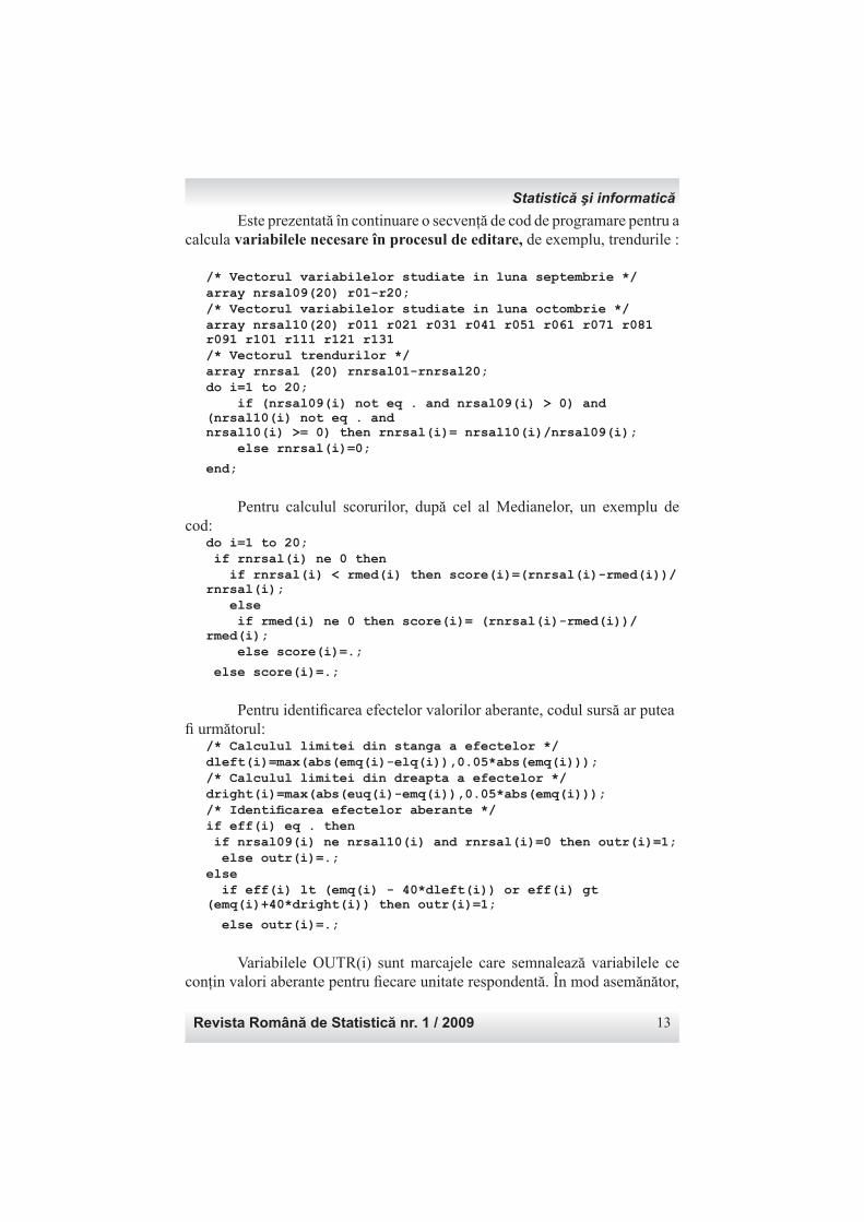
Este prezentată în continuare o secvenţă de cod de programare pentru a calcula variabilele necesare în procesul de editare, de exemplu, trendurile :
/* Vectorul variabilelor studiate in luna septembrie */ array nrsal09(20) r01-r20;/* Vectorul variabilelor studiate in luna octombrie */array nrsal10(20) r011 r021 r031 r041 r051 r061 r071 r081 r091 r101 r111 r121 r131 /* Vectorul trendurilor */array rnrsal (20) rnrsal01-rnrsal20; do i=1 to 20; if (nrsal09(i) not eq . and nrsal09(i) > 0) and (nrsal10(i) not eq . and nrsal10(i) >= 0) then rnrsal(i)= nrsal10(i)/nrsal09(i); else rnrsal(i)=0;
end;
Pentru calculul scorurilor, după cel al Medianelor, un exemplu de cod:
do i=1 to 20; if rnrsal(i) ne 0 then if rnrsal(i) < rmed(i) then score(i)=(rnrsal(i)-rmed(i))/rnrsal(i); else if rmed(i) ne 0 then score(i)= (rnrsal(i)-rmed(i))/rmed(i); else score(i)=.;
else score(i)=.;
Pentru identifi carea efectelor valorilor aberante, codul sursă ar putea fi următorul:
/* Calculul limitei din stanga a efectelor */dleft(i)=max(abs(emq(i)-elq(i)),0.05*abs(emq(i)));/* Calculul limitei din dreapta a efectelor */dright(i)=max(abs(euq(i)-emq(i)),0.05*abs(emq(i)));/* Identifi carea efectelor aberante */if eff(i) eq . then if nrsal09(i) ne nrsal10(i) and rnrsal(i)=0 then outr(i)=1; else outr(i)=.;else if eff(i) lt (emq(i) - 40*dleft(i)) or eff(i) gt (emq(i)+40*dright(i)) then outr(i)=1;
else outr(i)=.;
Variabilele OUTR(i) sunt marcajele care semnalează variabilele ce conţin valori aberante pentru fi ecare unitate respondentă. În mod asemănător,
Statistică şi informatică
Romanian Statistical Review nr. 1 / 200914
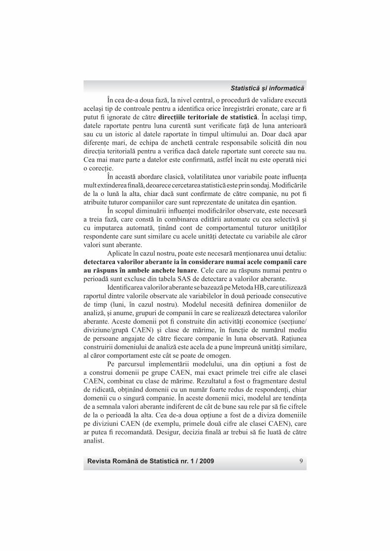
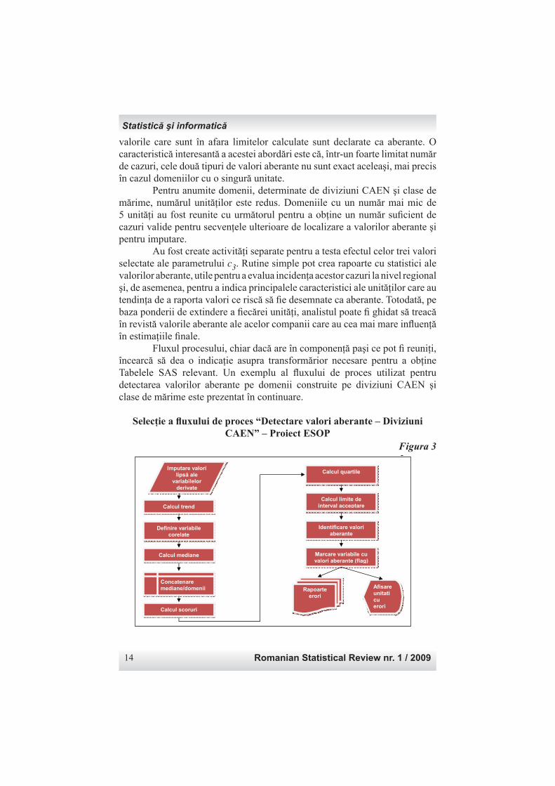
valorile care sunt în afara limitelor calculate sunt declarate ca aberante. O caracteristică interesantă a acestei abordări este că, într-un foarte limitat număr de cazuri, cele două tipuri de valori aberante nu sunt exact aceleaşi, mai precis în cazul domeniilor cu o singură unitate. Pentru anumite domenii, determinate de diviziuni CAEN şi clase de mărime, numărul unităţilor este redus. Domeniile cu un număr mai mic de 5 unităţi au fost reunite cu următorul pentru a obţine un număr sufi cient de cazuri valide pentru secvenţele ulterioare de localizare a valorilor aberante şi pentru imputare. Au fost create activităţi separate pentru a testa efectul celor trei valori selectate ale parametrului c3. Rutine simple pot crea rapoarte cu statistici ale valorilor aberante, utile pentru a evalua incidenţa acestor cazuri la nivel regional şi, de asemenea, pentru a indica principalele caracteristici ale unităţilor care au tendinţa de a raporta valori ce riscă să fi e desemnate ca aberante. Totodată, pe baza ponderii de extindere a fi ecărei unităţi, analistul poate fi ghidat să treacă în revistă valorile aberante ale acelor companii care au cea mai mare infl uenţă în estimaţiile fi nale. Fluxul procesului, chiar dacă are în componenţă paşi ce pot fi reuniţi, încearcă să dea o indicaţie asupra transformărior necesare pentru a obţine Tabelele SAS relevant. Un exemplu al fl uxului de proces utilizat pentru detectarea valorilor aberante pe domenii construite pe diviziuni CAEN şi clase de mărime este prezentat în continuare.
Selecţie a fl uxului de proces “Detectare valori aberante – Diviziuni CAEN” – Proiect ESOP
Figura 3Fig 3.
Calcul trend
Imputare valori
lips! ale
variabilelor
derivate
Definire variabile
corelate
Calcul mediane
Concatenare
mediane/domenii
Calcul scoruri
Calcul quartile
Calcul limite de
interval acceptare
Identificare valori
aberante
Marcare variabile cu
valori aberante (flag)
Rapoarte
erori
Afisare
unitati
cu
erori
Statistică şi informatică
Revista Română de Statistică nr. 1 / 2009 15
Descrierea Metodei FELLEGI-HOLT În orice cercetare statistică este necesară defi nirea unui set de condiţii de control, cât mai cuprinzător cu putinţă, pentru a fi ltra datele eronate încă din etapa de înregistrare a datelor în formularele anchetei. În etapa de editare automată (control automat) se utilizează acelaşi set de condiţii de control. Ele sunt utile după imputarea variabilelor cantitative metrice identifi cate ca având valori aberante. Metoda Fellegi-Holt indică faptul că datele trebuie să respecte toate condiţiile de control prin modifi carea valorilor variabilelor cu cea mai mică sumă posibilă a ponderilor de încredere. În termeni matematici, aşa cum se sugerează în [4], condiţiile de control pot fi clasifi cate în două mari categorii. Prima dintre ele poate implica mai multe variabile şi are o formă generală de tipul: 02,
10 <⋅+∑
=ji
n
jj yaa (13)
unde aj poate fi o constantă sau numele unei variabile auxiliare. Introducerea în defi niţia condiţiei de control a denumirii variabilei este o caracteristică extrem de importantă, folositoare pentru simplifi carea scrierii codului de programare în SAS. Utilizând yl,d ca limita inferioară a variabilei,
a0 = - yl,d şi =
=altfel
ijdacaa j ,0
,1. În cazul limitei superioare, avem
a0 = yu,d şi =−
=altfel
ijdacaa j ,0
,1.
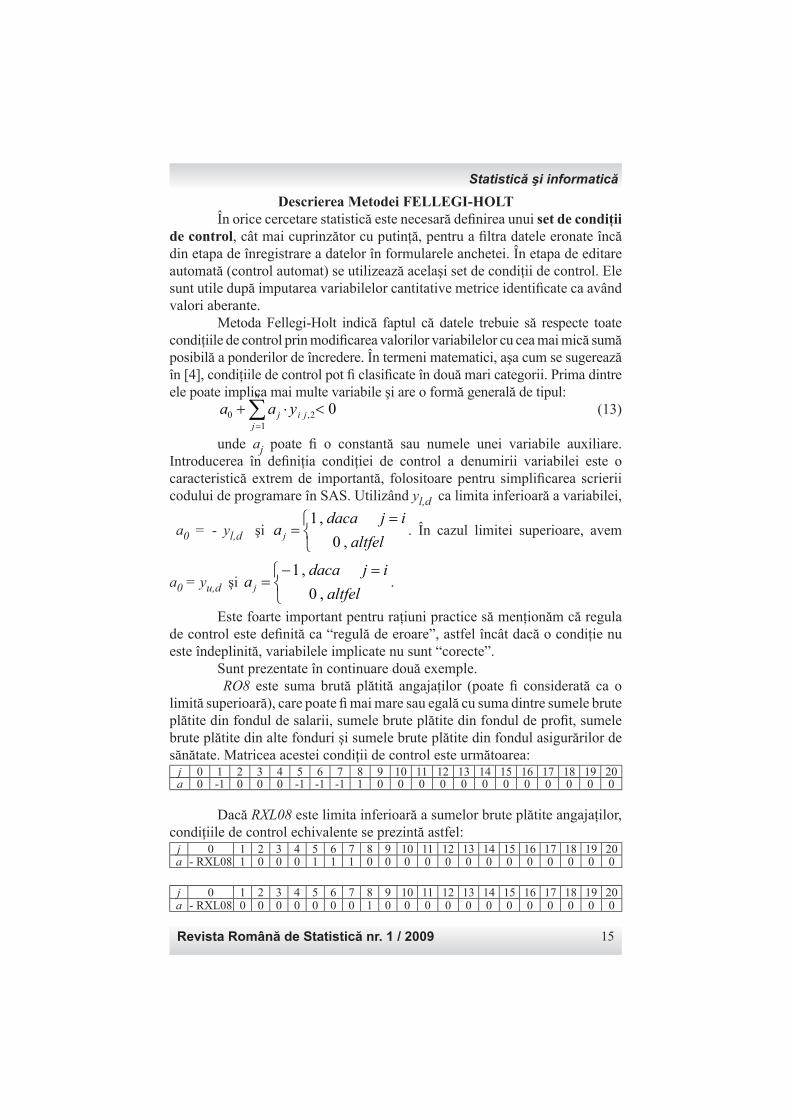
Este foarte important pentru raţiuni practice să menţionăm că regula de control este defi nită ca “regulă de eroare”, astfel încât dacă o condiţie nu este îndeplinită, variabilele implicate nu sunt “corecte”. Sunt prezentate în continuare două exemple. RO8 este suma brută plătită angajaţilor (poate fi considerată ca o limită superioară), care poate fi mai mare sau egală cu suma dintre sumele brute plătite din fondul de salarii, sumele brute plătite din fondul de profi t, sumele brute plătite din alte fonduri şi sumele brute plătite din fondul asigurărilor de sănătate. Matricea acestei condiţii de control este următoarea:
j 0 1 2 3 4 5 6 7 8 9 10 11 12 13 14 15 16 17 18 19 20a 0 -1 0 0 0 -1 -1 -1 1 0 0 0 0 0 0 0 0 0 0 0 0
Dacă RXL08 este limita inferioară a sumelor brute plătite angajaţilor, condiţiile de control echivalente se prezintă astfel:
j 0 1 2 3 4 5 6 7 8 9 10 11 12 13 14 15 16 17 18 19 20a - RXL08 1 0 0 0 1 1 1 0 0 0 0 0 0 0 0 0 0 0 0 0
j 0 1 2 3 4 5 6 7 8 9 10 11 12 13 14 15 16 17 18 19 20a - RXL08 0 0 0 0 0 0 0 1 0 0 0 0 0 0 0 0 0 0 0 0
Statistică şi informatică
Romanian Statistical Review nr. 1 / 200916
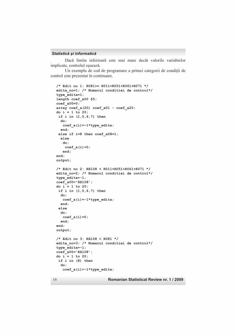
Dacă limita inferioară este mai mare decât valorile variabielor implicate, controlul eşuează. Un exemplu de cod de programare a primei categorii de condiţii de control este prezentat în continuare.
/* Edit no 1: R081>= R011+R051+R061+R071 */edita_no=1; /* Numarul conditiei de control*/type_edita=1;length coef_a00 $5;coef_a00=0;array coef_a(20) coef_a01 - coef_a20;do i = 1 to 20; if i in (1,5,6,7) then do; coef_a(i)=-1*type_edita; end; else if i=8 then coef_a08=1; else do; coef_a(i)=0; end;end;output;
/* Edit no 2: RXl08 < R011+R051+R061+R071 */edita_no=2; /* Numarul conditiei de control*/type_edita=-1;coef_a00=’RXl08’;do i = 1 to 20; if i in (1,5,6,7) then do; coef_a(i)=-1*type_edita; end; else do; coef_a(i)=0; end;end;output;
/* Edit no 3: RXl08 < R081 */edita_no=3; /* Numarul conditiei de control*/type_edita=-1;coef_a00=’RXl08’;do i = 1 to 20; if i in (8) then do; coef_a(i)=-1*type_edita;
Statistică şi informatică
Revista Română de Statistică nr. 1 / 2009 17
end; else do; coef_a(i)=0; end;end;output;
run;
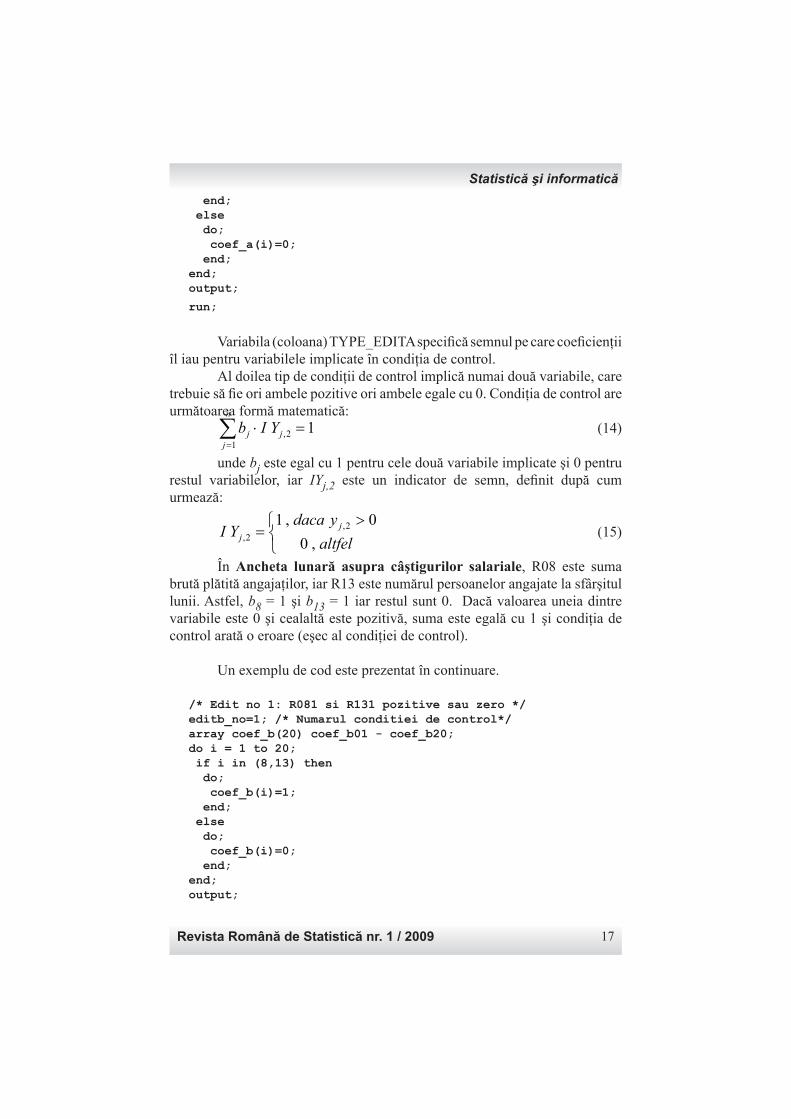
Variabila (coloana) TYPE_EDITA specifi că semnul pe care coefi cienţii îl iau pentru variabilele implicate în condiţia de control. Al doilea tip de condiţii de control implică numai două variabile, care trebuie să fi e ori ambele pozitive ori ambele egale cu 0. Condiţia de control are următoarea formă matematică: 1 2,
1
=⋅∑=
j
n
jj YIb (14)
unde bj este egal cu 1 pentru cele două variabile implicate şi 0 pentru restul variabilelor, iar IYj,2 este un indicator de semn, defi nit după cum urmează:
>
=altfel
ydacaYI j
j ,0
0,1 2,
2, (15) În Ancheta lunară asupra câştigurilor salariale, R08 este suma brută plătită angajaţilor, iar R13 este numărul persoanelor angajate la sfârşitul lunii. Astfel, b8 = 1 şi b13 = 1 iar restul sunt 0. Dacă valoarea uneia dintre variabile este 0 şi cealaltă este pozitivă, suma este egală cu 1 şi condiţia de control arată o eroare (eşec al condiţiei de control).
Un exemplu de cod este prezentat în continuare.
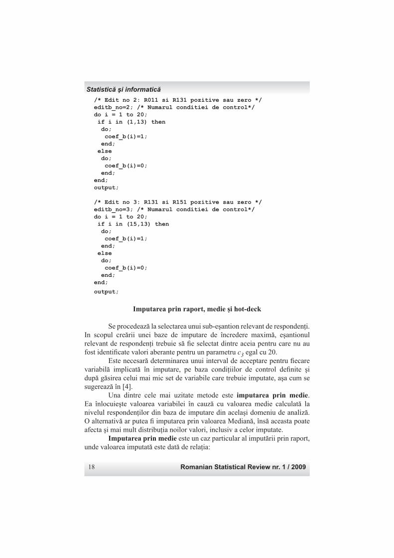
/* Edit no 1: R081 si R131 pozitive sau zero */editb_no=1; /* Numarul conditiei de control*/array coef_b(20) coef_b01 - coef_b20;do i = 1 to 20; if i in (8,13) then do; coef_b(i)=1; end; else do; coef_b(i)=0; end;end;output;
Statistică şi informatică
Romanian Statistical Review nr. 1 / 200918
/* Edit no 2: R011 si R131 pozitive sau zero */editb_no=2; /* Numarul conditiei de control*/do i = 1 to 20; if i in (1,13) then do; coef_b(i)=1; end; else do; coef_b(i)=0; end;end;output;
/* Edit no 3: R131 si R151 pozitive sau zero */editb_no=3; /* Numarul conditiei de control*/do i = 1 to 20; if i in (15,13) then do; coef_b(i)=1; end; else do; coef_b(i)=0; end;end;
output;
Imputarea prin raport, medie şi hot-deck
Se procedează la selectarea unui sub-eşantion relevant de respondenţi. In scopul creării unei baze de imputare de încredere maximă, eşantionul relevant de respondenţi trebuie să fi e selectat dintre aceia pentru care nu au fost identifi cate valori aberante pentru un parametru c3 egal cu 20. Este necesară determinarea unui interval de acceptare pentru fi ecare variabilă implicată în imputare, pe baza condiţiilor de control defi nite şi după găsirea celui mai mic set de variabile care trebuie imputate, aşa cum se sugerează în [4]. Una dintre cele mai uzitate metode este imputarea prin medie. Ea înlocuieşte valoarea variabilei în cauză cu valoarea medie calculată la nivelul respondenţilor din baza de imputare din acelaşi domeniu de analiză. O alternativă ar putea fi imputarea prin valoarea Mediană, însă aceasta poate afecta şi mai mult distribuţia noilor valori, inclusiv a celor imputate. Imputarea prin medie este un caz particular al imputării prin raport, unde valoarea imputată este dată de relaţia:
Statistică şi informatică
Revista Română de Statistică nr. 1 / 2009 19
jijji xRy ˆˆ ⋅= (16)
unde xij este valoarea unei variabile auxiliare (spre exemplu, numărul mediu al persoanelor ocupate, ea fi ind corelată cu plata sumelor brute) şi
∑∑
∈
∈=Si ji
Si ji
j x
yR r
ˆ . Desigur, dacă xij=1, obţinem specifi caţia imputării
prin medie. O altă metodă constă în imputarea valorilor invalide sau lipsă cu valori de la donatori găsiţi în acelaşi domeniu al bazei de imputare, din aceeaşi perioadă de timp, denumită imputare hot-deck. Pot exista cazuri în care valori pentru mai multe unităţi să fi e imputate cu o valoare de la acelaşi donator. Din acest motiv metoda este combinată cu imputarea prin donator aleator. Donatorii sunt aleşi complet aleator dintr-un domeniu de donatori, iar valoarea selectată înlocuieşte valoarea invalidă sau lipsă. Metoda este intensivă în termeni de programare şi timp de calculator, deoarece procesul de selecţie a donatorului trebuie să fi e repetat pentru toate unităţile cu date invalide sau lipsă. Dacă domeniul donatorilor nu este sufi cient de mare, procedura reuneşte primul domeniu identifi cat cu cel următor, până când este găsit un donator. Metoda este cunoscută în literatura de specialitate ca Metoda de imputare ierarhică hot-deck. Caracteristicile Anchetei lunare asupra câştigurilor salariale realizată de INS implică adaptarea metodei la modul în care sunt culese şi organizate datele. Întrucât algoritmul de detectare a valorilor aberante este restricţionat la nivelul rândurilor de total din tabelele SAS primare, se poate ridica o întrebare: dacă valorile aberante sunt găsite şi imputate, cum se poate translata valoarea imputată totală asupra cifrelor raportate de unitate pentru activitatea principală şi activităţile secundare ? Metoda cea mai facilă este de a imputa valorile parţiale utilzând raportul dintre valorile de origine ale termenilor sumei şi valoarea totală. Valorile aferente activităţii principale şi celor secundare pot fi calculate cu formula:
Tji
sjiTjisji y
yyy
,
, , , ˆˆ ⋅= (17)
unde s desemnează valorile corespunzătoare activităţilor principală şi secundare, iar T desemnează valorile pentru totaluri raportate pentru intreaga unitate statistică. Cerinţa ca valorile la nivel de unitate să fi e conforme cu regula de bază, adică valorile imputate pentru total să fi e egale cu suma valorilor aceleiaşi variabile raportată pentru activitatea principală şi cele secundare, dacă există,
Statistică şi informatică
Romanian Statistical Review nr. 1 / 200920
este extrem de importantă. În timpul calculelor, poziţiile zecimale pot cauza eşecul condiţiilor de control, deci va fi necesară multă atenţie atunci când aceste valori imputate sunt obţinute. Din nou, o soluţie facilă este de a reconstrui totalurile din termenii imputaţi. Intr-o manieră similară, valorile aberante pot fi marcate atunci când valoarea unei variabile pentru luna curentă pare a fi egală cu limita inferioară şi superioară, aşa cum sunt defi nite în (11) şi (12). Acest fapt este cauzat că trendul este egal cu trendul median, iar efectul şi scorul sunt egale cu zero. Însă valorile zecimale provoacă apariţia unei diferenţe, iar o funcţie FUZZ poate rezolva acest aparent paradox. Din nou, acest caz particular apare când în anumite activităţi (diviziuni CAEN) există o singură unitate – în principal companii de stat foarte mari – sau când defi nirea unei clase de mărime mult prea fi nă determină domenii cu o singură unitate. Este necesară o analiză atentă a acestor domenii înainte de lansarea procedurii de calcul al cuartilelor.
Concluzii
SAS Enterprise Guide oferă o platformă puternică de proiectare a fl uxurilor de proces separate pentru pregătirea datelor şi pentru a proceda la imputarea automată a datelor, utilizând metode bine cunoscute, potrivite pentru anchetele prin sondajele repetitive. În cursul dezvoltării proiectului, s-a considerat că statisticienii pot avea un control mult mai bun asupra tuturor etapelor procesului şi posibilitatea de a interveni pentru ajustări ad-hoc, spre exemplu în defi nirea domeniilor de analiză sau în producerea altor rapoarte relevante. Statisticianul poate programa rularea proiectului la o anumită dată şi oră, astfel încât să evalueze rezultatelor cât mai repede posibil, luând în considerare termenele stricte şi standardele de calitate. A fost necesar ca o parte din codul de programare să fi e scris în afara mediului SAS Enterprise Guide, spre exemplu pentru a programa etape SAS Data Step mai rapid. Utilizarea facilităţilor SAS EG de a importa codul SAS a permis legarea facilă cu diferite etape ale proiectului, ajutând în acest fel statisticianul să înţeleagă şi să controleze întregul proces. In stadiul său actual, proiectul SAS EG oferă funcţiile identifi care a valorilor aberante şi de localizare a erorilor pentru Ancheta lunară asupra câştigurilor salariale, lucrare realizată de Institutul Naţional de Statistică. Pentru viitor, sunt avute în vedere patru principale direcţii de dezvoltare: • Proiectarea unei interfeţe prietenoase pentru statistician ca să vizualizeze înregistrările şi variabilele marcate ca valori aberante şi să anuleze marcajul dacă este necesar; • Dezvoltarea unui macro SAS mai sofi sticat pentru a implementa
Statistică şi informatică
Revista Română de Statistică nr. 1 / 2009 21
metoda de imputare a celui mai apropiat donator; • Dezvoltarea unui proces separat de calculare a unui set cuprinzător de indicatori de calitate, util pentru realizarea rapoartelor de calitate; • Includerea tratării non-răspunsului total şi a procedurilor de extindere în proiect, pentru obţinerea rezutatelor fi nale ale anchetei.
Note 1.În engleză, Regulile de validare şi control sunt denumite “editing rules” sau “editing norms”, ceea ce, în traducere, ar putea fi numite “reguli” sau “norme de editare”. 2.Defi niţia EUROSTAT: Tipul de unitate de activitate (kind of activity unit: KAU) grupează toate părţile unei întreprinderi care contribuie la realizarea une activităţi la nivel de clasă (4 cifre) ale NACE Rev. 2 şi corespunde la una sau mai multe subdiviziuni operaţionale ale întreprinderii. Sistemul informaţional al întreprinderii trebuie să fi e capabil să indice sau să calculeze pentru fi ecare KAU cel puţin valoarea producţiei, consumul intermediar, costul manoperei, surplusul de operare, forţa de muncă şi formarea brută de capital.
*** Autorul mulţumeşte lui Rudi Seljak, de la Ofi ciul de Statistică al Republicii Slovenia, lui Philippe Brion de la INSEE-Franţa, Simonei Bonghez de la Reprezentanţa SAS România şi Dianei Hodor de la Institutul Naţional de Statistică pentru sfaturile, contribuţia şi sprijinul lor pentru punerea în practică şi dezvoltarea proiectului.
Bibliografi e selectivă [1] Fellegi, I.P. and Hold, D.: A Systematic Approach to Automatic Edit and Imputation, Journal of the American Statistical Association, Application Section, 71: 17-35, 1976 [2] Hidiroglou, M.A and Berthelot, J.M: Statistical Editing and Imputation for Periodic Business Surveys, Survey Methodology, 12(1): 73-83, June 1986, Statistics Canada [3] Hunt, J.W., Johnson, J.S. and King, C.S: Detecting Outliers in the Monthly Retail Trade Survey Using Hidiroglou-Berthelot Method, Proceedings of the Survey Research Methods Section, American Statistical Association (1999) [4] Seljak, R and Špeh, T. : Automatic Editing System for Two Short-Term Business Surveys, Supporting Paper presented at the Work Session on Statistical Data Editing, Conference of European Statisticians, Ottawa, 2005 [5] Recommended Practices for Editing and Imputation in Cross-Sectional Business Surveys, EDIMBUS Project, ISTAT, CBS, SFSO, August 2007
Statistică şi informatică
Romanian Statistical Review nr. 1 / 200922
AN APPLICATION OF DATA EDITING METHODS TO IMPROVE DATA QUALITY OF
SHORT-TERM BUSINESS STATISTICS
Dan Ion GHERGUŢ INSOMAR
Abstract
Improving statistical data quality is a key objective of the Romanian National Institute of Statistics (RNIS), and major efforts are devoted to produce and provide accurate data at the proper time for the proper users. It is, after all, the foundation of offi cial statistics credibility. In the production process of short-term business statistics—STS, specialists have to carefully judge the trade-off between data quality and usefulness: More accurate data means time and resources, but it is no longer of interest for users if the results are released too late. Bearing in mind the tight requirements, the Romanian National Institute of Statistics (RNIS) undertook several actions to reform the production process of STS. One step was to redefi ne the entire data collection and capturing process; the second one was to modernize the data processing instruments. In this second step, SAS® Enterprise Guide® is heavily used in several departments for data editing, imputation, grossing-up, and tabulation, in order to reduce the time till the release of offi cial results and to secure their overall quality. The paper gives a picture of the SAS® applications used in RNIS, implementing the recommended methods for data control and editing, applied in the area of short-term business surveys. Some considerations upon one method broadly used in the data editing process are presented, basically required for item-non-response treatment by means of classic imputation methods - mean value, hot-deck, historical data and, more seldom, cold-deck imputation – ensuring, also, the data-editing controls.
***
In the European Union, the production of monthly business statistics data (so called the short-term business statistics – STS) must comply with the provisions of the Council Regulation (EC) No 1165/98, amended by Regulation (EC) No 1158/2005 of the European Parliament and of the Council. The STS Regulation covers four major domains: industry, construction, retail trade and other services, defi ned according to the NACE classifi cation of activities (NACE rev.2). In addition to the STS Regulation, the STS requirements indicate the variables, periodicity, the level of details and the submission deadlines for the concerned variables to EUROSTAT. These deadlines vary from 15 days up to 2 months, depending on the type of required variable an on the group that each Member State belongs to, the group being defi ned by each country contribution to the value added obtained at EU level.
Statistics and IT
Revista Română de Statistică nr. 1 / 2009 23
Most often, the pressure of having the raw data at a reasonable date every month is diverted towards companies, which sometimes should fi ll-in the questionnaires some days before their fi nancial reports are closed, thus trying to gain some extra time for regional offi ces and central teams to capture the data, to perform primary validation, loading the central database and then to clean the data, to produce the required results and disseminate them. The companies have the possibility to revise their prior reported data on the occasion of the next monthly survey, but this still imply that all data must comply with precise and as comprehensive as possible editing rules. Even if the data-entry procedures are designed to fi ltrate the units that provided erroneous data, some of the data inconsistencies can be sought for only when the entire SAS table is available, giving the possibility to explore each unit’s historical data or to make comparisons within a certain analysis domain, given for example, by their economic activity and size class or geographical region. The urge to release the results as soon as possible after the reference month gives little time to recall the companies or to perform manual corrections if errors are found. In fact, the phase of data editing is one of the most time consuming after the raw data is captured and as bore some this activity might be, it is crucial for the quality of the results. Therefore, it is obvious that selective and automatic editing procedures are needed in order to cope with the short delays and the quality standards. Before the accession of Romania to the European Union, the Romanian National Statistical Institute (RNIS) started to implement the STS Regulation and in 2003 redesigned the entire data capturing and validation process within a PHARE National Program, having in the end the so called UNICA system. In general lines, the system comprised a Web-based data-entry application, which allows the regional offi ces to enter the data in a single central ORACLE data-base, to apply harmonized validation procedures and to revise the data till a specifi ed deadline each month. After this, central teams responsible for each area covered by the STS Regulation can extract the data and apply specifi c IT applications in order to produce the required statistics and afterwards, on one hand, to submit them to EUROSTAT and, on the other hand, to prepare the tabulations for national publications. In order to increase the data quality and to give the statisticians the possibility to respond more quickly to ad-hoc data requirements, the RNIS carried out in 2006 and 2007 a project with SAS Representative Offi ce Romania that resulted in a comprehensive set of SAS data marts extracted from the ORACLE central database. The next natural step was to start the development of automatic data editing procedures that could signifi cantly reduce the time to produce good quality results. As a pilot project, it was decided to build such procedures for the monthly survey on wages, which is one of the most sensible, in terms of its’ results, and most demanding in terms of details (both on economic activities and counties). This project was developed under SAS Enterprise Guide 4.0. This paper describes the fi rst steps taken to prepare the SAS tables extracted from the primary SAS tables in a suitable structure and the application of the Hidiroglou-Berthelot method to detect outliers (the H-B method) and the Fellegi-Holt method for localizing errors and data imputation. These methods are applied on two-months wages survey data (September and October 2006), based on recommendations given
Statistics and IT
Romanian Statistical Review nr. 1 / 200924
in [5] and the results of the application of the same methods obtained by the Statistical Offi ce of Republic of Slovenia, presented in [2]. In the second section an overview of the basic SAS tables on monthly wage survey and the SAS Enterprise Guide steps to produce the input SAS tables used in the following phases are given. The third section describes the models used to detect outliers, the corresponding sample code and some examples of the results. In the fourth section specifi cations on imputation methods used at RNIS are presented. The last section presents the main conclusions and the future developments of the project.
Description of primary SAS tables and preparation of input SAS tables
The primary SAS tables for the monthly survey on wages follow the philosophy of the data-entry applications used at RNIS for all statistical surveys: every questionnaire or statistical form is seen as a combination of “chapters” and within each “chapter” we have a set of rows and columns. In the case of the monthly survey on wages, there are two “chapters”. The fi rst chapter contains as rows the statistical variables on wages and salaries (a number of 12) and the second chapter contains the rows on number of employed persons and hours worked (in a number of 8). As columns, the SAS table includes the data on the main and secondary economic activities the company is engaged in. Thus, each record contains a combination of rows and columns. For instance, if we ask for the gross wage paid and the company, beside its main activity, has two other secondary activities, there will be a row (record) for the gross wages paid within the main activity and other two rows for each identifi ed secondary activity. In reality, each company has also a row that is the total of the other subsequent rows. Even if this is seen as an extra burden for the responding unit, the totals row is an important control key both for the company and for the statistical offi ce. In order to identify the Kind of Activity Units (KAU1) for all surveyed companies, the questionnaire is designed to collect data for the main activity and maximum 13 secondary activities. The number of secondary activities was derived from the experience of previous monthly and annual business surveys. In this way, for about 20,000 companies included in the monthly survey, the primary SAS table has roughly 5,500,000 rows. Each unit’s record contains all the cells determined by rows and columns, no matter how many activities it has – 1 or other 13. The main variables of the monthly primary SAS tables are: the survey month, Unit ID, identifi cation of questionnaire’s cell (indicating the corresponding row and column), the NACE class and the cell’s value. Only a limited number of companies have several secondary activities and, therefore, most off the cells are fi lled in with zero. After recoding the NACE values - because in the primary SAS table the NACE value for totals was marked with missing - and the variables’ names, in order to use them in following procedures as an array, the SAS table was transposed to construct separate rows for each company for total, main activity and existing secondary activities, together with a unique set of 20 observation variables. This structure was preferred against another possible solution, i.e. to have a unique row for each company, where as columns we could have a set of 20 observation variables multiplied with 14 activities (one main activity and 13 secondary) irrespective the number of secondary
Statistics and IT
Revista Română de Statistică nr. 1 / 2009 25
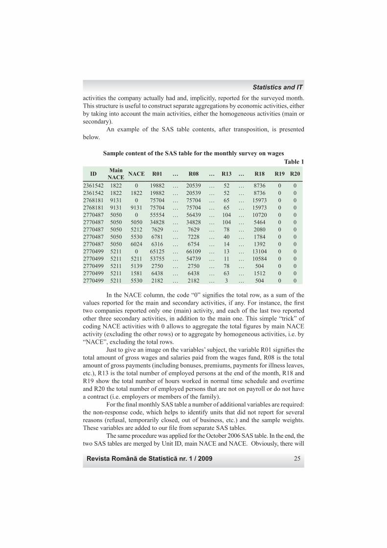
activities the company actually had and, implicitly, reported for the surveyed month. This structure is useful to construct separate aggregations by economic activities, either by taking into account the main activities, either the homogeneous activities (main or secondary). An example of the SAS table contents, after transposition, is presented below.
Sample content of the SAS table for the monthly survey on wagesTable 1
IDMain
NACENACE R01 … R08 … R13 … R18 R19 R20
2361542 1822 0 19882 … 20539 … 52 … 8736 0 02361542 1822 1822 19882 … 20539 … 52 … 8736 0 02768181 9131 0 75704 … 75704 … 65 … 15973 0 02768181 9131 9131 75704 … 75704 … 65 … 15973 0 02770487 5050 0 55554 … 56439 … 104 … 10720 0 02770487 5050 5050 34828 … 34828 … 104 … 5464 0 02770487 5050 5212 7629 … 7629 … 78 … 2080 0 02770487 5050 5530 6781 … 7228 … 40 … 1784 0 02770487 5050 6024 6316 … 6754 … 14 … 1392 0 02770499 5211 0 65125 … 66109 … 13 … 13104 0 02770499 5211 5211 53755 … 54739 … 11 … 10584 0 02770499 5211 5139 2750 … 2750 … 78 … 504 0 02770499 5211 1581 6438 … 6438 … 63 … 1512 0 02770499 5211 5530 2182 … 2182 … 3 … 504 0 0
In the NACE column, the code “0” signifi es the total row, as a sum of the values reported for the main and secondary activities, if any. For instance, the fi rst two companies reported only one (main) activity, and each of the last two reported other three secondary activities, in addition to the main one. This simple “trick” of coding NACE activities with 0 allows to aggregate the total fi gures by main NACE activity (excluding the other rows) or to aggregate by homogeneous activities, i.e. by “NACE”, excluding the total rows. Just to give an image on the variables’ subject, the variable R01 signifi es the total amount of gross wages and salaries paid from the wages fund, R08 is the total amount of gross payments (including bonuses, premiums, payments for illness leaves, etc.), R13 is the total number of employed persons at the end of the month, R18 and R19 show the total number of hours worked in normal time schedule and overtime and R20 the total number of employed persons that are not on payroll or do not have a contract (i.e. employers or members of the family). For the fi nal monthly SAS table a number of additional variables are required: the non-response code, which helps to identify units that did not report for several reasons (refusal, temporarily closed, out of business, etc.) and the sample weights. These variables are added to our fi le from separate SAS tables. The same procedure was applied for the October 2006 SAS table. In the end, the two SAS tables are merged by Unit ID, main NACE and NACE. Obviously, there will
Statistics and IT
Romanian Statistical Review nr. 1 / 200926
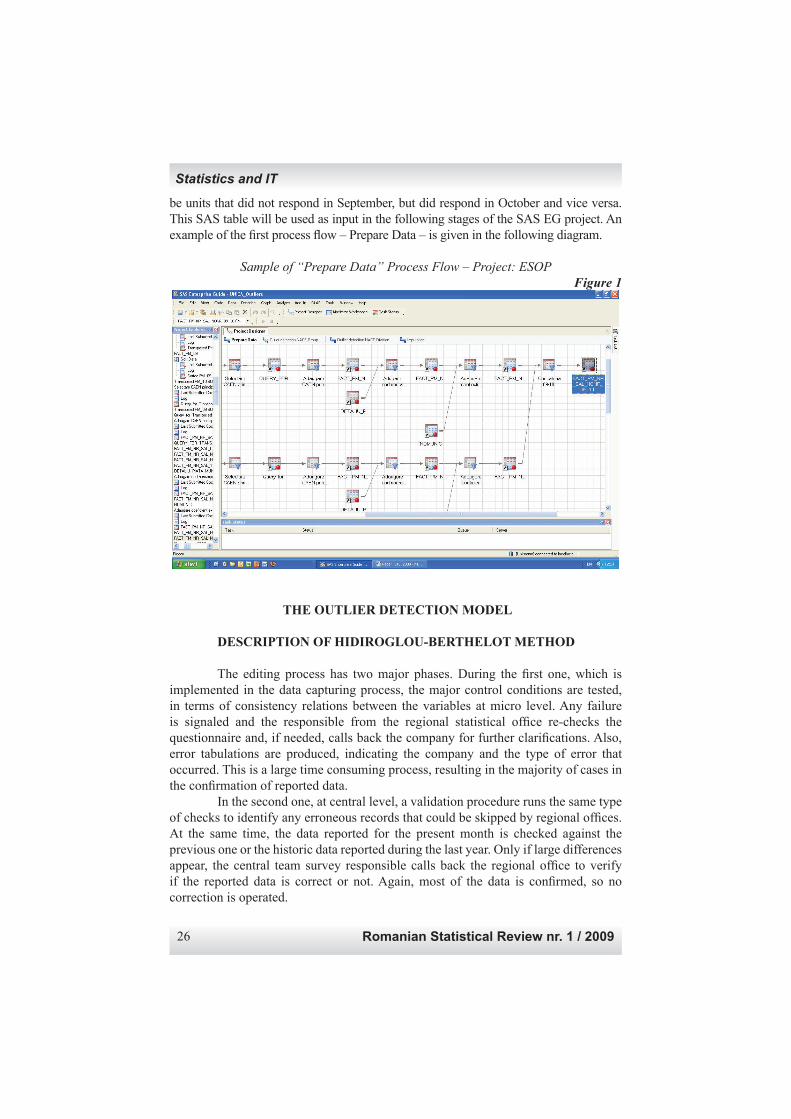
be units that did not respond in September, but did respond in October and vice versa. This SAS table will be used as input in the following stages of the SAS EG project. An example of the fi rst process fl ow – Prepare Data – is given in the following diagram.
Sample of “Prepare Data” Process Flow – Project: ESOP Figure 1
THE OUTLIER DETECTION MODEL
DESCRIPTION OF HIDIROGLOU-BERTHELOT METHOD
The editing process has two major phases. During the fi rst one, which is implemented in the data capturing process, the major control conditions are tested, in terms of consistency relations between the variables at micro level. Any failure is signaled and the responsible from the regional statistical offi ce re-checks the questionnaire and, if needed, calls back the company for further clarifi cations. Also, error tabulations are produced, indicating the company and the type of error that occurred. This is a large time consuming process, resulting in the majority of cases in the confi rmation of reported data. In the second one, at central level, a validation procedure runs the same type of checks to identify any erroneous records that could be skipped by regional offi ces. At the same time, the data reported for the present month is checked against the previous one or the historic data reported during the last year. Only if large differences appear, the central team survey responsible calls back the regional offi ce to verify if the reported data is correct or not. Again, most of the data is confi rmed, so no correction is operated.
Statistics and IT
Revista Română de Statistică nr. 1 / 2009 27
In this classical approach, the volatility of some variables can infl uence a lot the fi nal grossing-up, since we deal with a sample survey. Changes from one month to another, even confi rmed by the company, cannot be attributed to all the companies that the sampled unit represents. In order to diminish the infl uence of observed changes, a third phase is required, to combine selective and automatic editing and imputation, taking into account the behavior of all the respondent units that are similar with those units detected with outlier variables. Applied to our case, perhaps a detail should be mentioned: the detection of outliers takes into account only those companies that answered in the both monthly surveys. Therefore, those units responding only for one period are excluded from the SAS table. The detection of outliers is based on H-B method, which uses the ratio between the values of the observed variables in two consecutive time periods (months in our case). The model requires the defi nition of analysis domains, i.e. groups of companies within the detection of outliers is performed. These domains can be constructed by business activities (NACE headings) and size classes, based on the average number of persons employed by each company in the observed month. The rationale of the domain construction is to put together similar units, whose behavior is as homogeneous as possible. During the model implementation, one option was to construct domains by NACE groups, more exactly the fi rst three digits of the NACE class, combined with size classes. The result was a rather high fragmentation, obtaining domains with a very low number of respondents, even domains with only one company. In these small domains, the model tendency is to fl ag outliers no matter good or bad seem to be the fi gures from one period to another. The second option was to divide the domains by NACE division (i.e. fi rst two digits of NACE class), which could be recommended. Of course, the fi nal decision should be taken by the analyst. For the description of the model, some notations are needed. For any unit i, we have 20 variables yij,t, where j is the variable index (j = 1 ÷20) and t designates our two time periods (t = 1 and t = 2).The ratio of these two variables is called trend:
>
=
altfel
yisexistaydacay
y
t jijiji
ji
ji
,0
0 , 1, 1, 1,
2,
(1)
Within each domain, the unweighted median of these trends is computed:
djtmed )( , where d is the domain. Using the trends median, within the particular domain, for each unit and variable a score is computed, designated to ensure more symmetry of the tails of the trend distribution:
≥−
≤<−=
djjidjji
djjijidj
ji tmedtfitmedt
tmedtfittmeds
)( ,1)(/
)(0 ,/)(1
(2)
Statistics and IT
Romanian Statistical Review nr. 1 / 200928
If tij is zero, the corresponding score is not defi ned, which should mark implicitly these records as outliers. This should be quite natural if for the previous month the unit reported a non zero value for a certain variable, and zero for the next one, or vice-versa. In reality, this could occur, for instance in the case of illness payments or bonuses.A second transformation is performed, in order to combine the scores with magnitude of the analyzed data as effects: 1] ),( [max 2, 1,
cjijijiji yysE = (3)
where c1 is a tuning parameter with values between 0 and 1. If c1 is set to zero the effect yields to sij , omitting to consider the size of the unit. If it set to 1, the larger the value, the larger the infl uence on the determination of the outliers. In the literature, this parameter is set to 0.5.The next step is to calculate the scale of the left and right tail of the effects distribution. For this purpose we need to compute the effects’ quartiles within each particular domain for all our variables: EQ1, EQ2 and EQ3. The scales of the left and right tails are defi ned by:
],max[ 2212, QQQleftj EcEEd −= (4)
],max[ 2223, QQQrightj EcEEd −= (5)
The second part of the maximization function gives the possibility to prevent looking for correct data in regions too close the median. Also in practice, this tuning parameter is set to 0.05. If the effects are outside the interval
],[ ,32,32 rightjQleftjQ dcEdcE ⋅+⋅− (6)
the value of the corresponding variable is fl agged as outlier. The parameter c3 determines the width of the acceptance interval, with a maximum of 100. The literature indicates a recommended value of 40. As the parameter is set to larger values, the rejection area becomes smaller and the outlier fl ags show critical units and variables that should be reviewed. A set of three values of c3 were tested, following the approach suggested in [3]: 20, 40 and 50. Using a value of 20, the method declared 6,370 units having several variables marked as outliers, 6,013 for a value of 40 and 5,943 units for a value of 50. The outliers declared for c3 = 50 are generally suppressed from the imputation base and analyst review, qualifying them for automatic imputation. Nevertheless, in our case there are still implicit outliers marked due to zero values for the current month or, in small analysis domains, because of slight changes from one month to another. Irrespective the chosen parameter value, the analyst should review the outliers and override the fl ag if he or she considers the reported value as accurate, starting with the data set determined by the largest parameter value. In addition to outlier detection method based calculated effects, another
Statistics and IT
Revista Română de Statistică nr. 1 / 2009 29
solution is to defi ne bounds for each variable for each unit. For this purpose, a method is suggested in [4], consisting in inverse transformations. The scores lower and upper bounds are calculated as follows:
( ) 1 ),max( 2, 1,
,32, c
jiji
leftjQdl yy
dcEs
⋅−= (7)
( ) 1 ),max( 2, 1,
,32, c
jiji
rightjQdu yy
dcEs
⋅+= (8)
The lower and upper bound of ratio medians are:
)1(
)(,
l
djdl s
tmedt −= (9)
)1()(, udjdu stmedt +⋅= (10)
Finally, the lower and upper bound of each variable’s value are given by:
1, ,, jidldl yty ⋅= (11)
1, ,, jidudu yty ⋅= (12)
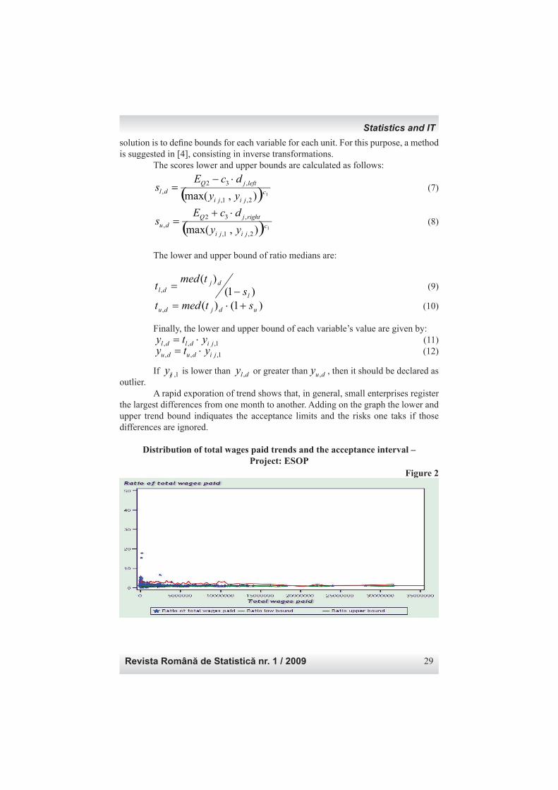
If 1,ijy is lower than dly , or greater than duy , , then it should be declared as outlier. A rapid exporation of trend shows that, in general, small enterprises register the largest differences from one month to another. Adding on the graph the lower and upper trend bound indiquates the acceptance limits and the risks one taks if those differences are ignored.
Distribution of total wages paid trends and the acceptance interval – Project: ESOP
Figure 2
Statistics and IT
Romanian Statistical Review nr. 1 / 200930
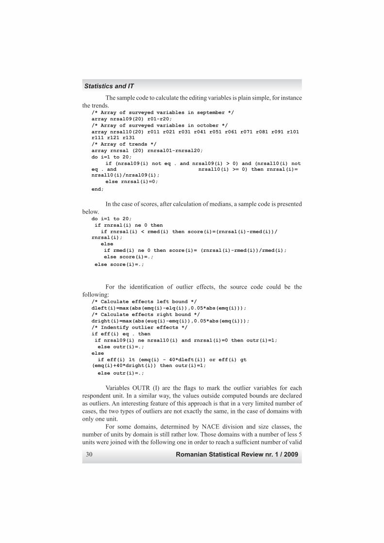
The sample code to calculate the editing variables is plain simple, for instance the trends.
/* Array of surveyed variables in september */ array nrsal09(20) r01-r20;/* Array of surveyed variables in october */array nrsal10(20) r011 r021 r031 r041 r051 r061 r071 r081 r091 r101 r111 r121 r131 /* Array of trends */array rnrsal (20) rnrsal01-rnrsal20; do i=1 to 20; if (nrsal09(i) not eq . and nrsal09(i) > 0) and (nrsal10(i) not eq . and nrsal10(i) >= 0) then rnrsal(i)= nrsal10(i)/nrsal09(i); else rnrsal(i)=0;
end;
In the case of scores, after calculation of medians, a sample code is presented below.
do i=1 to 20; if rnrsal(i) ne 0 then if rnrsal(i) < rmed(i) then score(i)=(rnrsal(i)-rmed(i))/rnrsal(i); else if rmed(i) ne 0 then score(i)= (rnrsal(i)-rmed(i))/rmed(i); else score(i)=.;
else score(i)=.;
For the identifi cation of outlier effects, the source code could be the following:
/* Calculate effects left bound */dleft(i)=max(abs(emq(i)-elq(i)),0.05*abs(emq(i)));/* Calculate effects right bound */dright(i)=max(abs(euq(i)-emq(i)),0.05*abs(emq(i)));/* Indentify outlier effects */if eff(i) eq . then if nrsal09(i) ne nrsal10(i) and rnrsal(i)=0 then outr(i)=1; else outr(i)=.;else if eff(i) lt (emq(i) - 40*dleft(i)) or eff(i) gt (emq(i)+40*dright(i)) then outr(i)=1;
else outr(i)=.;
Variables OUTR (I) are the fl ags to mark the outlier variables for each respondent unit. In a similar way, the values outside computed bounds are declared as outliers. An interesting feature of this approach is that in a very limited number of cases, the two types of outliers are not exactly the same, in the case of domains with only one unit. For some domains, determined by NACE division and size classes, the number of units by domain is still rather low. Those domains with a number of less 5 units were joined with the following one in order to reach a suffi cient number of valid
Statistics and IT
Revista Română de Statistică nr. 1 / 2009 31
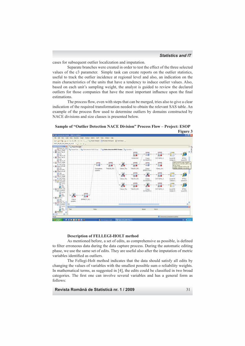
cases for subsequent outlier localization and imputation. Separate branches were created in order to test the effect of the three selected values of the c3 parameter. Simple task can create reports on the outlier statistics, useful to track the outlier incidence at regional level and also, an indication on the main characteristics of the units that have a tendency to induce outlier values. Also, based on each unit’s sampling weight, the analyst is guided to review the declared outliers for those companies that have the most important infl uence upon the fi nal estimations. The process fl ow, even with steps that can be merged, tries also to give a clear indication of the required transformation needed to obtain the relevant SAS table. An example of the process fl ow used to determine outliers by domains constructed by NACE divisions and size classes is presented below.
Sample of “Outlier Detection NACE Division” Process Flow – Project: ESOPFigure 3
Description of FELLEGI-HOLT method As mentioned before, a set of edits, as comprehensive as possible, is defi ned to fi lter erroneous data during the data capture process. During the automatic editing phase, we use the same set of edits. They are useful also after the imputation of metric variables identifi ed as outliers. The Fellegi-Holt method indicates that the data should satisfy all edits by changing the values of variables with the smallest possible sum o reliability weights. In mathematical terms, as suggested in [4], the edits could be classifi ed in two broad categories. The fi rst one can involve several variables and has a general form as follows:
Statistics and IT
Romanian Statistical Review nr. 1 / 200932
02, 1
0 <⋅+∑=
ji
n
jj yaa (13)
where aj could be a constant or a name of one to the auxiliary variables. The inclusion in the edit defi nition of the variable name is a very important feature of this model defi nition, useful to simplify the SAS ® programming code. Using yl,d as the
lower bound of variable yij,2, a0 = - yl,d and =
=altfel
ijdacaa j ,0
,1. In the case of
the upper bound, then we have a0 = yu,d and =−
=altfel
ijdacaa j ,0
,1.
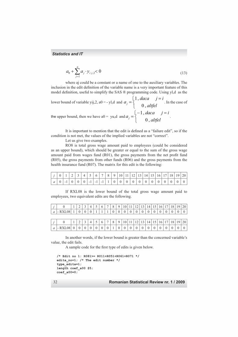
It is important to mention that the edit is defi ned as a “failure edit”, so if the condition is not met, the values of the implied variables are not “correct”. Let us give two examples. RO8 is total gross wage amount paid to employees (could be considered as an upper bound), which should be greater or equal to the sum of the gross wage amount paid from wages fund (R01), the gross payments from the net profi t fund (R05), the gross payments from other funds (R06) and the gross payments from the health insurance fund (R07). The matrix for this edit is the following:
j 0 1 2 3 4 5 6 7 8 9 10 11 12 13 14 15 16 17 18 19 20
a 0 -1 0 0 0 -1 -1 -1 1 0 0 0 0 0 0 0 0 0 0 0 0
If RXL08 is the lower bound of the total gross wage amount paid to employees, two equivalent edits are the following.
j 0 1 2 3 4 5 6 7 8 9 10 11 12 13 14 15 16 17 18 19 20
a - RXL08 1 0 0 0 1 1 1 0 0 0 0 0 0 0 0 0 0 0 0 0
j 0 1 2 3 4 5 6 7 8 9 10 11 12 13 14 15 16 17 18 19 20
a - RXL08 0 0 0 0 0 0 0 1 0 0 0 0 0 0 0 0 0 0 0 0
In another words, if the lower bound is greater than the concerned variable’s value, the edit fails. A sample code for the fi rst type of edits is given below.
/* Edit no 1: R081>= R011+R051+R061+R071 */edita_no=1; /* The edit number */type_edita=1;length coef_a00 $5;coef_a00=0;
Statistics and IT
Revista Română de Statistică nr. 1 / 2009 33
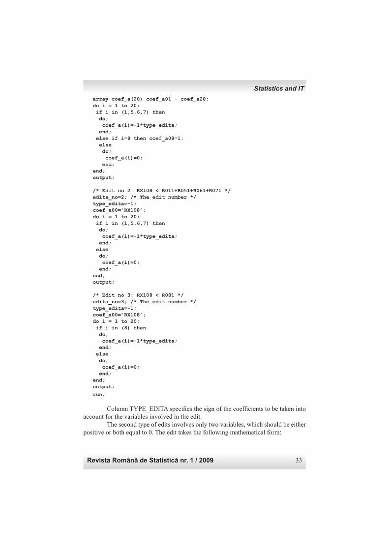
array coef_a(20) coef_a01 - coef_a20;do i = 1 to 20; if i in (1,5,6,7) then do; coef_a(i)=-1*type_edita; end; else if i=8 then coef_a08=1; else do; coef_a(i)=0; end;end;output;
/* Edit no 2: RXl08 < R011+R051+R061+R071 */edita_no=2; /* The edit number */type_edita=-1;coef_a00=’RXl08’;do i = 1 to 20; if i in (1,5,6,7) then do; coef_a(i)=-1*type_edita; end; else do; coef_a(i)=0; end;end;output;
/* Edit no 3: RXl08 < R081 */edita_no=3; /* The edit number */type_edita=-1;coef_a00=’RXl08’;do i = 1 to 20; if i in (8) then do; coef_a(i)=-1*type_edita; end; else do; coef_a(i)=0; end;end;output;
run;
Column TYPE_EDITA specifi es the sign of the coeffi cients to be taken into account for the variables involved in the edit. The second type of edits involves only two variables, which should be either positive or both equal to 0. The edit takes the following mathematical form:
Statistics and IT
Romanian Statistical Review nr. 1 / 200934
1 2,1
=⋅∑=
j
n
jj YIb
(14) where bj equals 1 for the two involved variables and 0 for the rest and IYj,2 is a sign indicator, defi ned as follows:
>
=altfel
ydacaYI j
j ,0
0,1 2,
2,
(15) As an example, in our monthly wage survey, R08 is the total gross wage amount paid to employees and R13 is the number of persons employed at the end of the month. Therefore, b8 = 1 and b13 = 1 and the rest are 0. If one variable is 0 and the other is positive, the sum yields 1 and the edit shows a failure condition. A sample code is given below.
/* Edit no 1: R081 and R131 positive or zero */editb_no=1; /* The edit number */array coef_b(20) coef_b01 - coef_b20;do i = 1 to 20; if i in (8,13) then do; coef_b(i)=1; end; else do; coef_b(i)=0; end;end;output;
/* Edit no 2: R011 and R131 positive or zero */editb_no=2; /* The edit number */do i = 1 to 20; if i in (1,13) then do; coef_b(i)=1; end; else do; coef_b(i)=0; end;end;output;
/* Edit no 3: R131 and R151 positive or zero */editb_no=3; /* The edit number */do i = 1 to 20; if i in (15,13) then do; coef_b(i)=1; end; else do;
Statistics and IT
Revista Română de Statistică nr. 1 / 2009 35
coef_b(i)=0; end;end;output;
/* Edit no 4: R011 and R161 positive or zero */editb_no=4; /* The edit number */do i = 1 to 20; if i in (1,16) then do; coef_b(i)=1; end; else do; coef_b(i)=0; end;end;
output;
Imputation methods Ratio, mean and HOT-DECK imputation For imputation purposes, a relevant sample of respondents must be selected. In order to give maximum reliability of the imputation base, the relevant sample is selected among respondents that were not declared as outliers for a c3 parameter equal 20. As suggested in [4], an acceptance interval has to be determined for each variable involved in imputation, based on defi ned edits and after fi nding the smallest set of variables to be imputed. One method often used is the mean imputation. It imputes the value of the concerned variable with the mean value computed among the respondents from the imputation base in the same analysis domain. An alternative could be the median value, but this could affect the distribution. The mean imputation method is special case of ratio imputation, where the imputed value is given by
jijji xRy ˆˆ ⋅= (16)
where xij is the value of an auxiliary variable (for instance the mean number of persons employed, being correlated with the gross wage payments) and
∑∑
∈
∈=Si ji
Si ji
j x
yR r
ˆ . Of course, if xij=1, we get the specifi cation of mean
imputation. Another method is to impute invalid or missing data with values from a donor found in the same domain of the imputation base, for the same period of time, called hot-deck imputation. There are cases when values for several units could be imputed with the same donor value. That is why this method is combined with random donor
Statistics and IT
Romanian Statistical Review nr. 1 / 200936
imputation. The donors are chosen completely at random from the donors’ domain and the selected value replaces the missing or invalid data. This method is rather intensive, since the donor selection process must be repeated for all units with invalid data. Also, if the donor domain is not large enough, the procedure collapses the fi rst identifi ed domain with the next one, until a donor is found. Literature labels this method as hierarchical hot-deck imputation. The specifi c features of the RNIS monthly survey on wages complicate a little bit the picture. As the outlier detection algorithm is restricted to total rows in the primary SAS table, a question may arise: if outlier values are found and therefore imputed, how to translate the imputed total value upon the unit’s reported fi gures for the main and secondary activities? The easiest solution is to impute the subsequent values using the original ratios between the terms of the sum and the total value. The values of the related main and secondary activities could be calculated as follows:
Tji
sjiTjisji y
yyy
,
, , , ˆˆ ⋅= (17)
where s designates the values corresponding to the main and secondary activities and T designates the values for the totals, reported for the entire statistical unit. One major issue is the requirement for these values, at unit level, to comply with the basic condition, i.e. the imputed value for totals to be equal with the sum of values for the same variables reported for the main and secondary activities. During calculation, decimal digits can cause the failure of this edit, so care should be taken when these imputed values are computed. Again, one easy solution is to reconstruct the totals from the imputed terms. In a similar way, outliers may occur when the variable’s value for the current month seems to be equal with the lower and upper bounds as defi ned in (11) and (12). This is due to the fact that the trend is equal with the median trend and the corresponding effect and score are 0. Decimal digits cause this difference and a FUZZ function could solve it. Again, this is a particular case when in some activities (NACE divisions) there are single units – mainly state companies – or a too refi ned size class defi nition creates domains with only one unit. A careful analysis of the resulted domains should be undertaken before starting the procedures that creates the quartiles.
Conclusions SAS Enterprise Guide provides a powerful platform to design separate process fl ows to prepare data and to proceed to automatic data editing imputation, using well-known methods suitable for repetitive sample surveys. In the development of this project, it was considered that statisticians could have a better control upon all data processing stages, having also the possibility to intervene for ad-hoc adjustments, for instance in the defi nition of domains or to produce other relevant reports. Also, the statistician can schedule the project to run on a specifi ed data and hour, so to assess the results as soon as possible, considering the tight deadlines and quality standards. Nevertheless, some code had to be written outside SAS Enterprise Guide,
Statistics and IT
Revista Română de Statistică nr. 1 / 2009 37
just to program SAS Data Steps faster. Using the SAS Enterprise Guide facilities to import SAS code, it was easy to link with different project steps, so to help statistician to understand and to control the process fl ow. In it’s present state, the SAS Enterprise Guide project delivers outlier identifi cation, error localization and imputation for the monthly survey on wages carried out by Romanian National Statistical Institute. As for the future, four main developments are envisaged: • to design a friendly interface that allows the statistician to visualize the records and the variables marked as outliers and to override the fl ag if necessary; • to develop a more sophisticated SAS macro to implement the nearest neighbor imputation method; • to develop a separate process fl ow to compute a comprehensive set of quality indicators, useful for required quality reports; • to include the total non-response treatement and grossing-up procedures to produce the fi nal survey results.
Note 1. EUROSTAT defi nition: The kind of activity unit (KAU) groups all the parts of an enterprise contributing to the performance of an activity at class level (4- digits) of NACE Rev. 2 and corresponds to one or more operational subdivisions of the enterprise. The enterprise’s information system must be capable of indicating or calculating for each KAU at least the production value, intermediate consumption, manpower costs, the operating surplus and employment and gross fi xed capital formation.
ACKNOWLEDGMENTS The author would like to thank Rudi Seljak, Statistical Offi ce of the Republic of Slovenia, Philippe Brion, INSEE-France and Simona Bonghez, SAS Representative Offi ce - Romania for their inputs, contribution and support to the implementation and development of this project.
References [1] Fellegi, I.P. and Hold, D.: A Systematic Approach to Automatic Edit and Imputation, Journal of the American Statistical Association, Application Section, 71: 17-35, 1976 [2] Hidiroglou, M.A and Berthelot, J.M: Statistical Editing and Imputation for Periodic Business Surveys, Survey Methodology, 12(1): 73-83, June 1986, Statistics Canada [3] Hunt, J.W., Johnson, J.S. and King, C.S: Detecting Outliers in the Monthly Retail Trade Survey Using Hidiroglou-Berthelot Method, Proceedings of the Survey Research Methods Section, American Statistical Association (1999) [4] Seljak, R and Špeh, T. : Automatic Editing System for Two Short-Term Business Surveys, Supporting Paper presented at the Work Session on Statistical Data Editing, Conference of European Statisticians, Ottawa, 2005 [5] Recommended Practices for Editing and Imputation in Cross-Sectional Business Surveys, EDIMBUS Project, ISTAT, CBS, SFSO, August 2007
Statistics and IT
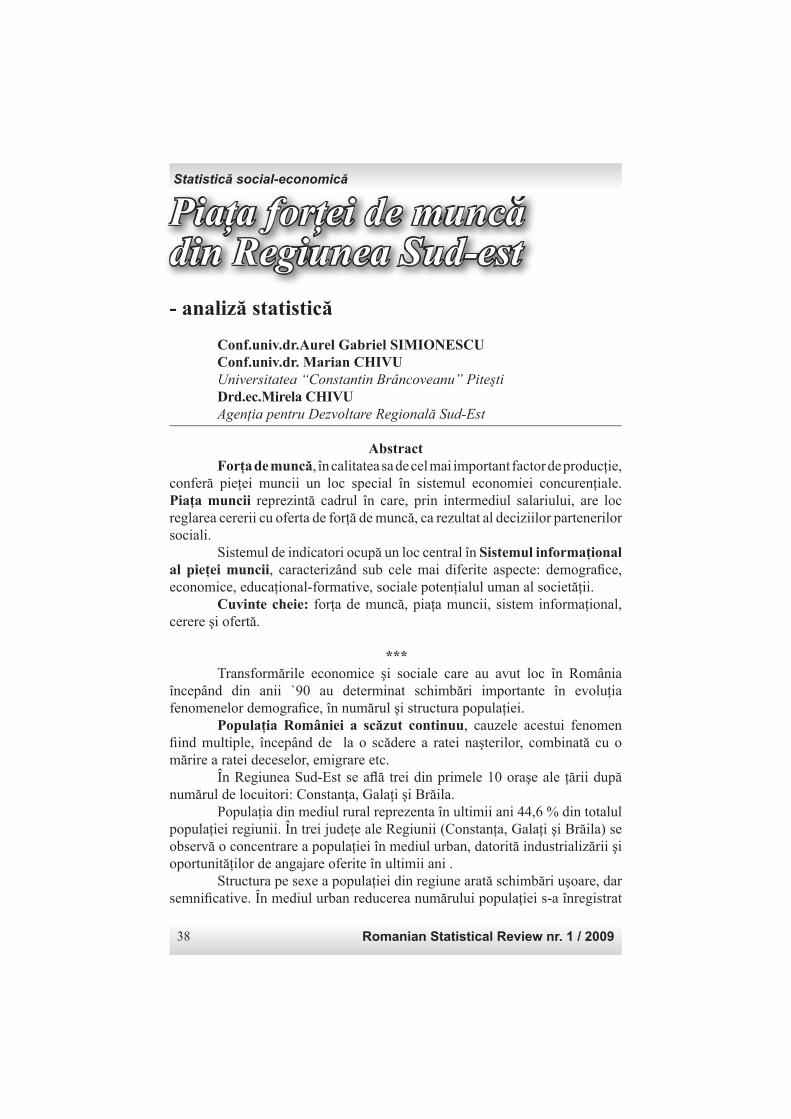
Romanian Statistical Review nr. 1 / 200938
Piaţa forţei de muncă din Regiunea Sud-est- analiză statistică
Conf.univ.dr.Aurel Gabriel SIMIONESCU Conf.univ.dr. Marian CHIVU Universitatea “Constantin Brâncoveanu” Piteşti Drd.ec.Mirela CHIVU Agenţia pentru Dezvoltare Regională Sud-Est
Abstract Forţa de muncă, în calitatea sa de cel mai important factor de producţie, conferă pieţei muncii un loc special în sistemul economiei concurenţiale. Piaţa muncii reprezintă cadrul în care, prin intermediul salariului, are loc reglarea cererii cu oferta de forţă de muncă, ca rezultat al deciziilor partenerilor sociali. Sistemul de indicatori ocupă un loc central în Sistemul informaţional al pieţei muncii, caracterizând sub cele mai diferite aspecte: demografi ce, economice, educaţional-formative, sociale potenţialul uman al societăţii. Cuvinte cheie: forţa de muncă, piaţa muncii, sistem informaţional, cerere şi ofertă.
*** Transformările economice şi sociale care au avut loc în România începând din anii `90 au determinat schimbări importante în evoluţia fenomenelor demografi ce, în numărul şi structura populaţiei. Populaţia României a scăzut continuu, cauzele acestui fenomen fi ind multiple, începând de la o scădere a ratei naşterilor, combinată cu o mărire a ratei deceselor, emigrare etc. În Regiunea Sud-Est se afl ă trei din primele 10 oraşe ale ţării după numărul de locuitori: Constanţa, Galaţi şi Brăila. Populaţia din mediul rural reprezenta în ultimii ani 44,6 % din totalul populaţiei regiunii. În trei judeţe ale Regiunii (Constanţa, Galaţi şi Brăila) se observă o concentrare a populaţiei în mediul urban, datorită industrializării şi oportunităţilor de angajare oferite în ultimii ani . Structura pe sexe a populaţiei din regiune arată schimbări uşoare, dar semnifi cative. În mediul urban reducerea numărului populaţiei s-a înregistrat
Statistică social-economică
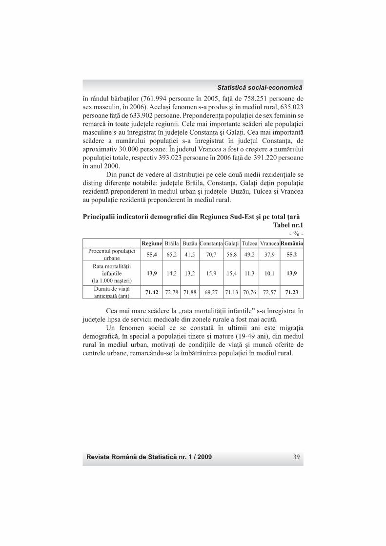
Revista Română de Statistică nr. 1 / 2009 39
în rândul bărbaţilor (761.994 persoane în 2005, faţă de 758.251 persoane de sex masculin, în 2006). Acelaşi fenomen s-a produs şi în mediul rural, 635.023 persoane faţă de 633.902 persoane. Preponderenţa populaţiei de sex feminin se remarcă în toate judeţele regiunii. Cele mai importante scăderi ale populaţiei masculine s-au înregistrat în judeţele Constanţa şi Galaţi. Cea mai importantă scădere a numărului populaţiei s-a înregistrat în judeţul Constanţa, de aproximativ 30.000 persoane. În judeţul Vrancea a fost o creştere a numărului populaţiei totale, respectiv 393.023 persoane în 2006 faţă de 391.220 persoane în anul 2000. Din punct de vedere al distribuţiei pe cele două medii rezidenţiale se disting diferenţe notabile: judeţele Brăila, Constanţa, Galaţi deţin populaţie rezidentă preponderent în mediul urban şi judeţele Buzău, Tulcea şi Vrancea au populaţie rezidentă preponderent în mediul rural.
Principalii indicatorii demografi ci din Regiunea Sud-Est şi pe total ţară Tabel nr.1
- % - Regiune Brăila Buzău Constanţa Galaţi Tulcea Vrancea România
Procentul populaţiei urbane
55,4 65,2 41,5 70,7 56,8 49,2 37,9 55.2
Rata mortalităţii infantile
(la 1.000 naşteri)13,9 14,2 13,2 15,9 15,4 11,3 10,1 13,9
Durata de viaţă anticipată (ani)
71,42 72,78 71,88 69,27 71,13 70,76 72,57 71,23
Cea mai mare scădere la „rata mortalităţii infantile” s-a înregistrat în judeţele lipsa de servicii medicale din zonele rurale a fost mai acută. Un fenomen social ce se constată în ultimii ani este migraţia demografi că, în special a populaţiei tinere şi mature (19-49 ani), din mediul rural în mediul urban, motivaţi de condiţiile de viaţă şi muncă oferite de centrele urbane, remarcându-se la îmbătrânirea populaţiei în mediul rural.
Statistică social-economică
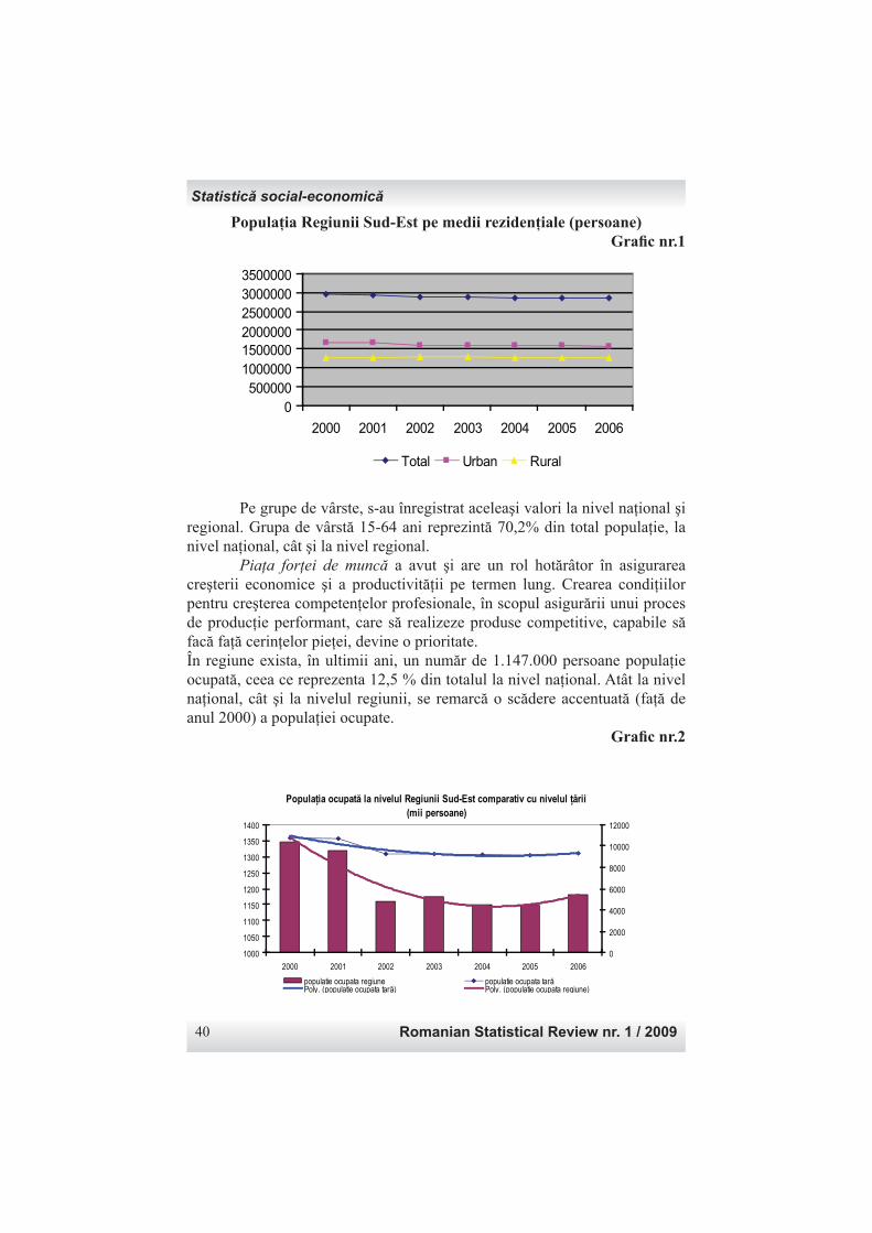
Romanian Statistical Review nr. 1 / 200940
Populaţia Regiunii Sud-Est pe medii rezidenţiale (persoane)Grafi c nr.1
0
500000
1000000
1500000
2000000
2500000
3000000
3500000
2000 2001 2002 2003 2004 2005 2006
Total Urban Rural
Pe grupe de vârste, s-au înregistrat aceleaşi valori la nivel naţional şi regional. Grupa de vârstă 15-64 ani reprezintă 70,2% din total populaţie, la nivel naţional, cât şi la nivel regional. Piaţa forţei de muncă a avut şi are un rol hotărâtor în asigurarea creşterii economice şi a productivităţii pe termen lung. Crearea condiţiilor pentru creşterea competenţelor profesionale, în scopul asigurării unui proces de producţie performant, care să realizeze produse competitive, capabile să facă faţă cerinţelor pieţei, devine o prioritate.În regiune exista, în ultimii ani, un număr de 1.147.000 persoane populaţie ocupată, ceea ce reprezenta 12,5 % din totalul la nivel naţional. Atât la nivel naţional, cât şi la nivelul regiunii, se remarcă o scădere accentuată (faţă de anul 2000) a populaţiei ocupate.
Grafi c nr.2
Populaţia ocupată la nivelul Regiunii Sud-Est comparativ cu nivelul ţării
(mii persoane)
1000
1050
1100
1150
1200
1250
1300
1350
1400
2000 2001 2002 2003 2004 2005 2006
0
2000
4000
6000
8000
10000
12000
populatie ocupata regiune populatie ocupata tarăPoly. (populatie ocupata tară) Poly. (populatie ocupata regiune)
Statistică social-economică
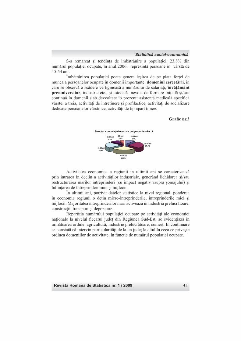
Revista Română de Statistică nr. 1 / 2009 41
S-a remarcat şi tendinţa de îmbătrânire a populaţiei, 23,8% din numărul populaţiei ocupate, în anul 2006, reprezintă persoane în vârstă de 45-54 ani. Îmbătrânirea populaţiei poate genera ieşirea de pe piaţa forţei de muncă a persoanelor ocupate în domenii importante: domeniul cercetării, în care se observă o scădere vertiginoasă a numărului de salariaţi, învăţământ pre/universitar, industrie etc., şi totodată nevoia de formare iniţială şi/sau continuă în domenii slab dezvoltate în prezent: asistenţă medicală specifi că vârstei a treia, activităţi de întreţinere şi profi lactice, activităţi de socializare dedicate persoanelor vârstnice, activităţi de tip «part time».
Grafi c nr.3
55-64 ani9,8%
45-54 ani23,8%
35-44 ani25,6%
25-34 ani27,1%
15-24 ani9,1%
65+ani4,6%
Structura populaţiei ocupate pe grupe de vârstă
Activitatea economica a regiunii in ultimii ani se caracterizează prin intrarea în declin a activităţilor industriale, generând lichidarea şi/sau restructurarea marilor întreprinderi (cu impact negativ asupra şomajului) şi înfi inţarea de întreprinderi mici şi mijlocii. În ultimii ani, potrivit datelor statistice la nivel regional, ponderea în economia regiunii o deţin micro-întreprinderile, întreprinderile mici şi mijlocii. Majoritatea întreprinderilor mari activează în industria prelucrătoare, construcţii, transport şi depozitare. Repartiţia numărului populaţiei ocupate pe activităţi ale economiei naţionale la nivelul fi ecărui judeţ din Regiunea Sud-Est, se evidenţiază în următoarea ordine: agricultură, industrie prelucrătoare, comerţ. În continuare se constată că intervin particularităţi de la un judeţ la altul în ceea ce priveşte ordinea domeniilor de activitate, în funcţie de numărul populaţiei ocupate.
Statistică social-economică
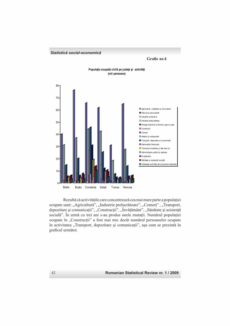
Romanian Statistical Review nr. 1 / 200942
Grafi c nr.4
0
10
20
30
40
50
60
70
80
Brăila Buzău Constanţa Galaţi Tulcea Vrancea
Populaţia ocupată civilă pe judeţe şi activităţi
(mii persoane)
Agricultură, v ânătoare şi silv icultură
Pescuit şi piscicultură
Industrie ex tractiv ă
Industrie prelucrătoare
Energie electrică şi termică, gaze şi apă
Construcţii
Comerţ
Hoteluri şi restaurante
Transport, depozitare şi comunicaţii
Intermedieri financiare
Tranzacţii imobiliare şi alte serv icii
Administraţie publică şi apărare
Înv ăţământ
Sănătate şi asistenţă socială
Celelalate activ ităţi ale economiei naţionale
Rezultă că activităţile care concentrează cea mai mare parte a populaţiei ocupate sunt: „Agricultură”, „Industrie prelucrătoare”, „Comerţ” , „Transport, depozitare şi comunicaţii”, „Construcţii”, „Învăţământ”, „Sănătate şi asistenţă socială”. În urmă cu trei ani s-au produs unele mutaţii. Numărul populaţiei ocupate în „Construcţii” a fost mai mic decât numărul persoanelor ocupate în activitatea „Transport, depozitare şi comunicaţii”, aşa cum se prezintă în grafi cul următor.
Statistică social-economică
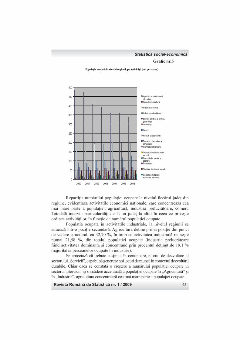
Revista Română de Statistică nr. 1 / 2009 43
Grafi c nr.5
Populaţia ocupată la nivelul regiunii, pe activităţi (mii persoane)
0
50
100
150
200
250
300
350
400
450
500
2000 2001 2002 2003 2004 2005 2006
Agricultură, vânătoare şisilviculturăPescuit şi piscicultură
Industrie extractivă
Industrie prelucrătoare
Energie electrică şi termică,gaze şi apăConstrucţii
Comerţ
Hoteluri şi restaurante
Transport, depozitare şicomunicaţiiIntermedieri financiare
Tranzacţii imobiliare şi alteserviciiAdministraţie publică şiapărareÎnvăţământ
Sănătate şi asistenţă socială
Celelalte activităţi aleeconomiei naţionale
Repartiţia numărului populaţiei ocupate la nivelul fi ecărui judeţ din regiune, evidenţiază activităţile economiei naţionale, care concentrează cea mai mare parte a populaţiei: agricultură, industria prelucrătoare, comerţ. Totodată intervin particularităţi de la un judeţ la altul în ceea ce priveşte ordinea activităţilor, în funcţie de numărul populaţiei ocupate. Populaţia ocupată în activităţile industriale, la nivelul regiunii se situează într-o poziţie secundară. Agricultura deţine prima poziţie din punct de vedere structural, cu 32,70 %, în timp ce activitatea industrială reuneşte numai 21,58 %, din totalul populaţiei ocupate (industria prelucrătoare fi ind activitatea dominantă şi concentrând prin procentul deţinut de 19,1 % majoritatea persoanelor ocupate în industrie). Se apreciază că trebuie susţinut, în continuare, efortul de dezvoltare al sectorului „Servicii”, capabil să genereze noi locuri de muncă în contextul dezvoltării durabile. Chiar dacă se constată o creştere a numărului populaţiei ocupate în sectorul „Servicii” şi o scădere accentuată a populaţiei ocupate în „Agricultură” şi în „Industrie”, agricultura concentrează cea mai mare parte a populaţiei ocupate.
Statistică social-economică
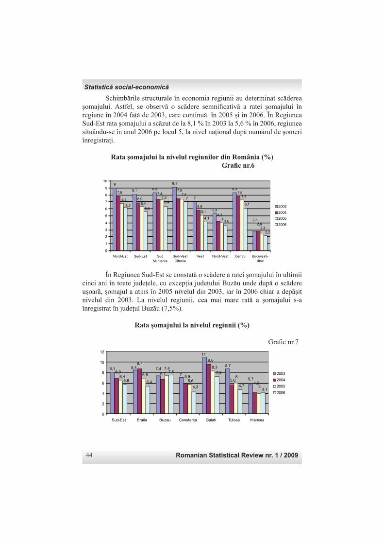
Schimbările structurale în economia regiunii au determinat scăderea şomajului. Astfel, se observă o scădere semnifi cativă a ratei şomajului în regiune în 2004 faţă de 2003, care continuă în 2005 şi în 2006. În Regiunea Sud-Est rata şomajului a scăzut de la 8,1 % în 2003 la 5,6 % în 2006, regiunea situându-se în anul 2006 pe locul 5, la nivel naţional după numărul de şomeri înregistraţi.
Rata şomajului la nivelul regiunilor din România (%) Grafi c nr.6
9
8,1 8,3
9,1
7
8,3
5,4
2,8
7,8
5,8
7,8
4,2
2,8
7,57,4
6,9
2,4
7,3
5,1
7,47,3
6,4
6,8
4
2,2
6,1
3,64,1
76,4
5,66,2
0
1
2
3
4
5
6
7
8
9
10
Nord-Est Sud-Est Sud
Muntenia
Sud-Vest
Oltenia
Vest Nord-Vest Centru Bucuresti-
Ilfov
2003
2004
2005
2006
În Regiunea Sud-Est se constată o scădere a ratei şomajului în ultimii cinci ani în toate judeţele, cu excepţia judeţului Buzău unde după o scădere uşoară, şomajul a atins în 2005 nivelul din 2003, iar în 2006 chiar a depăşit nivelul din 2003. La nivelul regiunii, cea mai mare rată a şomajului s-a înregistrat în judeţul Buzău (7,5%).
Rata şomajului la nivelul regiunii (%)
Grafi c nr.7
5,7
7,48,18,7
11
7
8,5
8,7
4,25,6
9,6
5,96,7
6,97,4
4
6
8,3
5,6
6,86,4
4,14,7
7,2
4,3
7,5
5,45,6
0
2
4
6
8
10
12
Sud-Est Braila Buzau Constanta Galati Tulcea Vrancea
2003
2004
2005
2006
Romanian Statistical Review nr. 1 / 200944
Statistică social-economică
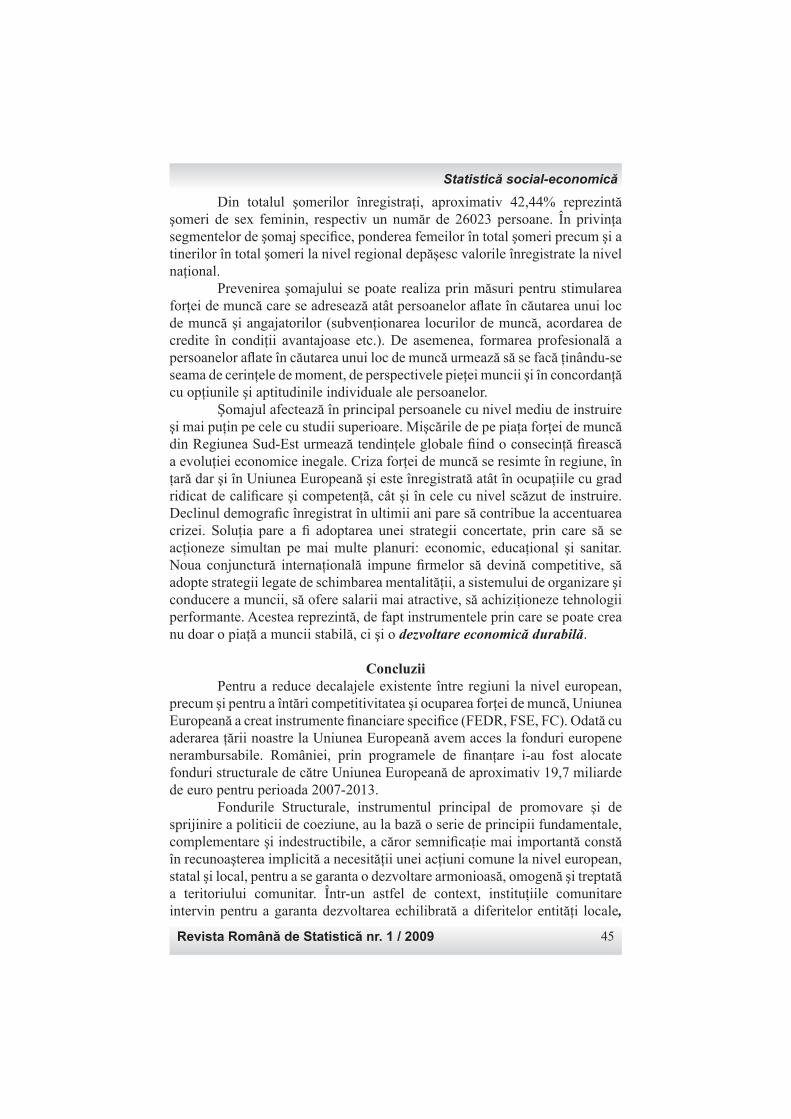
Din totalul şomerilor înregistraţi, aproximativ 42,44% reprezintă şomeri de sex feminin, respectiv un număr de 26023 persoane. În privinţa segmentelor de şomaj specifi ce, ponderea femeilor în total şomeri precum şi a tinerilor în total şomeri la nivel regional depăşesc valorile înregistrate la nivel naţional. Prevenirea şomajului se poate realiza prin măsuri pentru stimularea forţei de muncă care se adresează atât persoanelor afl ate în căutarea unui loc de muncă şi angajatorilor (subvenţionarea locurilor de muncă, acordarea de credite în condiţii avantajoase etc.). De asemenea, formarea profesională a persoanelor afl ate în căutarea unui loc de muncă urmează să se facă ţinându-se seama de cerinţele de moment, de perspectivele pieţei muncii şi în concordanţă cu opţiunile şi aptitudinile individuale ale persoanelor. Şomajul afectează în principal persoanele cu nivel mediu de instruire şi mai puţin pe cele cu studii superioare. Mişcările de pe piaţa forţei de muncă din Regiunea Sud-Est urmează tendinţele globale fi ind o consecinţă fi rească a evoluţiei economice inegale. Criza forţei de muncă se resimte în regiune, în ţară dar şi în Uniunea Europeană şi este înregistrată atât în ocupaţiile cu grad ridicat de califi care şi competenţă, cât şi în cele cu nivel scăzut de instruire. Declinul demografi c înregistrat în ultimii ani pare să contribue la accentuarea crizei. Soluţia pare a fi adoptarea unei strategii concertate, prin care să se acţioneze simultan pe mai multe planuri: economic, educaţional şi sanitar. Noua conjunctură internaţională impune fi rmelor să devină competitive, să adopte strategii legate de schimbarea mentalităţii, a sistemului de organizare şi conducere a muncii, să ofere salarii mai atractive, să achiziţioneze tehnologii performante. Acestea reprezintă, de fapt instrumentele prin care se poate crea nu doar o piaţă a muncii stabilă, ci şi o dezvoltare economică durabilă.
Concluzii Pentru a reduce decalajele existente între regiuni la nivel european, precum şi pentru a întări competitivitatea şi ocuparea forţei de muncă, Uniunea Europeană a creat instrumente fi nanciare specifi ce (FEDR, FSE, FC). Odată cu aderarea ţării noastre la Uniunea Europeană avem acces la fonduri europene nerambursabile. României, prin programele de fi nanţare i-au fost alocate fonduri structurale de către Uniunea Europeană de aproximativ 19,7 miliarde de euro pentru perioada 2007-2013. Fondurile Structurale, instrumentul principal de promovare şi de sprijinire a politicii de coeziune, au la bază o serie de principii fundamentale, complementare şi indestructibile, a căror semnifi caţie mai importantă constă în recunoaşterea implicită a necesităţii unei acţiuni comune la nivel european, statal şi local, pentru a se garanta o dezvoltare armonioasă, omogenă şi treptată a teritoriului comunitar. Într-un astfel de context, instituţiile comunitare intervin pentru a garanta dezvoltarea echilibrată a diferitelor entităţi locale,
Revista Română de Statistică nr. 1 / 2009 45
Statistică social-economică
Romanian Statistical Review nr. 1 / 200946
ori de câte ori acestea, datorită limitelor lor sau carenţelor administrative, nu pot acţiona. Cele două interpretări furnizează justifi cări diverse pentru intervenţia din partea nivelelor de guvernare «superioare». Se apreciază că trebuie promovată o reformă a bugetului naţional care să permită o integrare a procesului de planifi care, prioritizare şi cheltuire, atât a resurselor interne, cât şi a celor europene.
Bibliografi e
- Isaic-Maniu, Al., Mitruţ, C., Voineagu, V., Statistică pentru managementul afacerilor, Ediţia a II-a, Editura Economică, Bucureşti, 1998 - Lilea, E., Goschin Z., Vătui, M., Boldeanu, D., Statistică, Editura ASE, Bucureşti, 2001 - *** Planul de Dezoltare Regională al Regiunii Sud-Est, 2007-2013, Agenţia pentru Dezvoltare Regională Sud-Est - *** Programul Operaţional Sectorial Dezvoltarea Resurselor Umane 2007-2013 - *** Programul Operaţional Regional 2007-2013 - *** Strategia Lisabona, Comisia Europeană - *** Biroul European de Statistică, EUROSTAT, 2008 - *** Revista Română de Statistică, INS, Colecţia 2004-2008 - *** Anuarul Statistic al României, ediţiile 2001-2007 - www.ec.europa.eu - www.infoeuropa.ro
THE LABOR MARKET IN THE SOUTH- EAST REGION
- Statistical analysis -
PhD Senior Lecturer Aurel Gabriel SIMIONESCU PhD Senior Lecturer Marian CHIVU “Constantin Brâncoveanu” University, Pitesti PhD Candidate, Economist Mirela CHIVU Regional Development Agency South East
Employment is one of the most important factors of production, labor market has a special place in the competitive economy. Labor markets through salary adjusting by the supply and demand of manpower is a result of decisions made by the employers. The indicators play an important part of the central information system in the labor markets characterized by the different aspects - demographic, economic, educational-training, social potential of human society. Keywords: employment, labor market, information system, application and offer.
Statistică social-economică
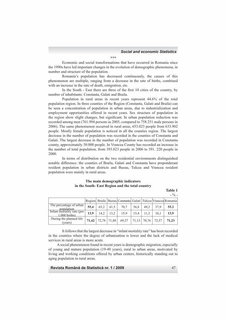
Revista Română de Statistică nr. 1 / 2009 47
*** Economic and social transformations that have occurred in Romania since the 1990s have led important changes in the evolution of demographic phenomena, in number and structure of the population. Romania’s population has decreased continuously, the causes of this phenomenon are multiple, ranging from a decrease in the rate of births, combined with an increase in the rate of death, emigration, etc. In the South - East there are three of the fi rst 10 cities of the country, by number of inhabitants: Constanta, Galati and Braila. Population in rural areas in recent years represent 44.6% of the total population region. In three counties of the Region (Constanta, Galati and Braila) can be seen a concentration of population in urban areas, due to industrialization and employment opportunities offered in recent years. Sex structure of population in the region show slight changes, but signifi cant. In urban population reduction was recorded among men (761.994 persons in 2005, compared to 758.251 male persons in 2006). The same phenomenon occurred in rural areas, 653.023 people from 633.902 people. Mostly female population is noticed in all the counties region. The largest decrease in the number of population was recorded in the counties of Constanta and Galati. The largest decrease in the number of population was recorded in Constanta county, approximately 30.000 people. In Vrancea County has recorded an increase in the number of total population, from 393.023 people in 2006 to 391. 220 people in 2000. In terms of distribution on the two residential environments distinguished notable difference: the counties of Braila, Galati and Constanta have preponderant resident population in urban districts and Buzau, Tulcea and Vrancea resident population were mainly in rural areas.
The main demographic indicators in the South- East Region and the total country
Table 1- % -
Region Braila Buzau Constanta Galati Tulcea Vrancea RomaniaThe percentage of urban
population55,4 65,2 41,5 70,7 56,8 49,2 37,9 55.2
Infant mortality rate (per 1.000 births)
13,9 14,2 13,2 15,9 15,4 11,3 10,1 13,9
During the planned life (years)
71,42 72,78 71,88 69,27 71,13 70,76 72,57 71,23
It follows that the largest decrease in “infant mortality rate” has been recorded in the counties where the degree of urbanization is lower and the lack of medical services in rural areas is more acute. A social phenomenon found in recent years is demographic migration, especially of young and mature population (19-49 years), rural to urban areas, motivated by living and working conditions offered by urban centers, historically standing out to aging population in rural areas.
Social and economic Statistics
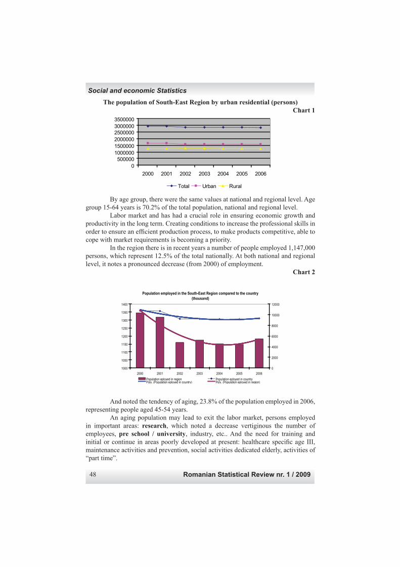
Romanian Statistical Review nr. 1 / 200948
The population of South-East Region by urban residential (persons)Chart 1
0
500000
1000000
1500000
2000000
2500000
3000000
3500000
2000 2001 2002 2003 2004 2005 2006
Total Urban Rural
By age group, there were the same values at national and regional level. Age group 15-64 years is 70.2% of the total population, national and regional level. Labor market and has had a crucial role in ensuring economic growth and productivity in the long term. Creating conditions to increase the professional skills in order to ensure an effi cient production process, to make products competitive, able to cope with market requirements is becoming a priority. In the region there is in recent years a number of people employed 1,147,000 persons, which represent 12.5% of the total nationally. At both national and regional level, it notes a pronounced decrease (from 2000) of employment.
Chart 2
Population employed in the South-East Region compared to the country (thousand)
1000
1050
1100
1150
1200
1250
1300
1350
1400
2000 2001 2002 2003 2004 2005 2006
0
2000
4000
6000
8000
10000
12000
Population eployed in region Population eployed in countryPoly. (Population eployed in country) Poly. (Population eployed in region)
And noted the tendency of aging, 23.8% of the population employed in 2006, representing people aged 45-54 years. An aging population may lead to exit the labor market, persons employed in important areas: research, which noted a decrease vertiginous the number of employees, pre school / university, industry, etc.. And the need for training and initial or continue in areas poorly developed at present: healthcare specifi c age III, maintenance activities and prevention, social activities dedicated elderly, activities of “part time”.
Social and economic Statistics
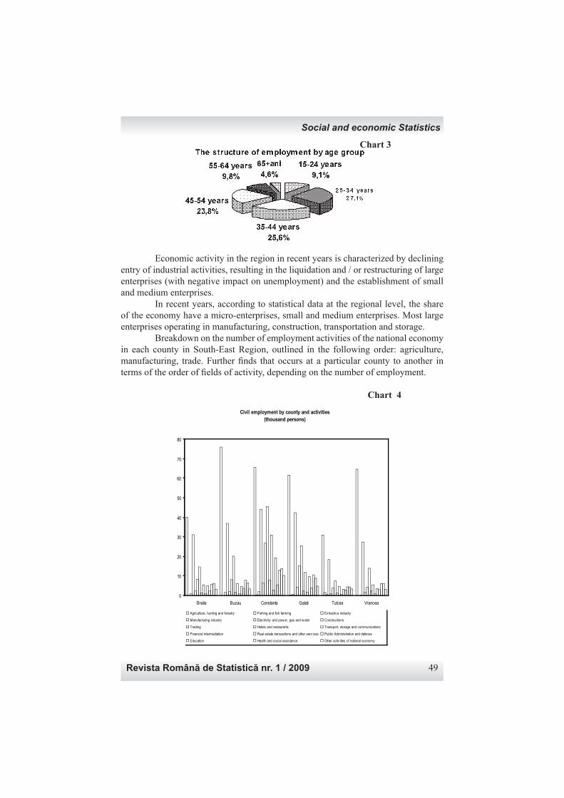
Revista Română de Statistică nr. 1 / 2009 49
Chart 3
Economic activity in the region in recent years is characterized by declining entry of industrial activities, resulting in the liquidation and / or restructuring of large enterprises (with negative impact on unemployment) and the establishment of small and medium enterprises. In recent years, according to statistical data at the regional level, the share of the economy have a micro-enterprises, small and medium enterprises. Most large enterprises operating in manufacturing, construction, transportation and storage. Breakdown on the number of employment activities of the national economy in each county in South-East Region, outlined in the following order: agriculture, manufacturing, trade. Further fi nds that occurs at a particular county to another in terms of the order of fi elds of activity, depending on the number of employment.
Chart 4
Civil employment by county and activities
(thousand persons)
0
10
20
30
40
50
60
70
80
Braila Buzau Constanta Galati Tulcea Vrancea
Agriculture, hunting and forestry Fishing and fish farming Ex tractiv e industry
Manufacturing industry Electricity and pow er, gas and w ater Constructions
Trading Hotels and restaurants Transport, storage and communications
Financial intermediation Real estate transactions and other serv ices Public Administration and defense
Education Health and social assistance Other activ ities of national economy
Social and economic Statistics
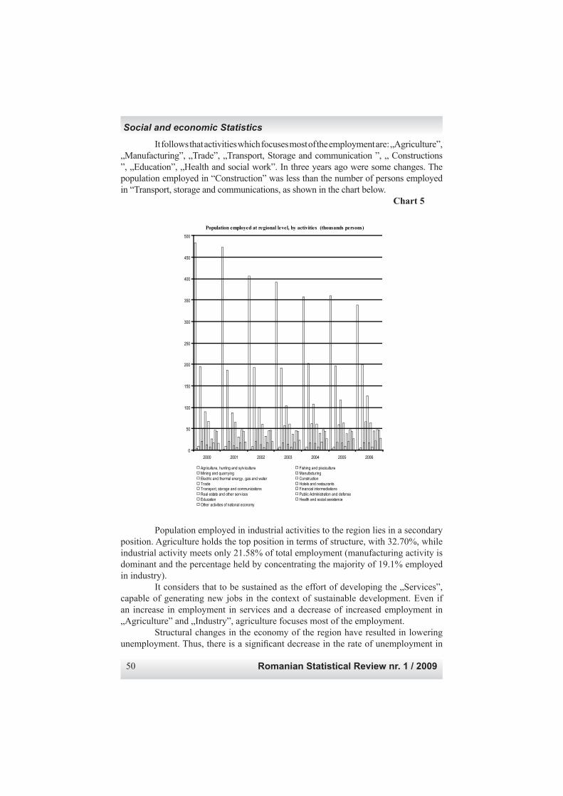
Romanian Statistical Review nr. 1 / 200950
It follows that activities which focuses most of the employment are: „Agriculture”, „Manufacturing”, „Trade”, „Transport, Storage and communication ”, „ Constructions ”, „Education”, „Health and social work”. In three years ago were some changes. The population employed in “Construction” was less than the number of persons employed in “Transport, storage and communications, as shown in the chart below. Chart 5
Population employed at regional level, by activities (thousands persons)
0
50
100
150
200
250
300
350
400
450
500
2000 2001 2002 2003 2004 2005 2006
Agriculture, hunting and sylviculture Fishing and piscicultureMining and quarrying ManufacturingElectric and thermal energy, gas and water ConstructionTrade Hotels and restaurantsTransport, storage and communications Financial intermediationsReal estate and other services Public Administration and defenseEducation Health and social assistanceOther activities of national economy
Population employed in industrial activities to the region lies in a secondary position. Agriculture holds the top position in terms of structure, with 32.70%, while industrial activity meets only 21.58% of total employment (manufacturing activity is dominant and the percentage held by concentrating the majority of 19.1% employed in industry). It considers that to be sustained as the effort of developing the „Services”, capable of generating new jobs in the context of sustainable development. Even if an increase in employment in services and a decrease of increased employment in „Agriculture” and „Industry”, agriculture focuses most of the employment. Structural changes in the economy of the region have resulted in lowering unemployment. Thus, there is a signifi cant decrease in the rate of unemployment in
Social and economic Statistics
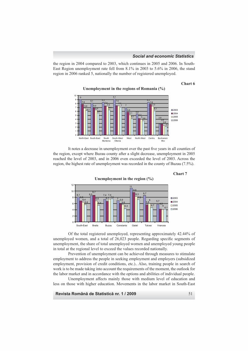
Revista Română de Statistică nr. 1 / 2009 51
the region in 2004 compared to 2003, which continues in 2005 and 2006. In South-East Region unemployment rate fell from 8.1% in 2003 to 5.6% in 2006, the stand region in 2006 ranked 5, nationally the number of registered unemployed.
Chart 6Unemployment in the regions of Romania (%)
9
8,1 8,3
9,1
7
8,3
5,4
2,8
7,8
5,8
7,8
4,2
2,8
7,57,4
6,9
2,4
7,3
5,1
7,47,3
6,4
6,8
4
2,2
6,1
3,64,1
76,4
5,66,2
0
1
2
3
4
5
6
7
8
9
10
North-East South-East South
Muntenia
South-West
Oltenia
West North-West Centru Bucharest-
Ilfov
2003
2004
2005
2006
It notes a decrease in unemployment over the past fi ve years in all counties of the region, except where Buzau county after a slight decrease, unemployment in 2005 reached the level of 2003, and in 2006 even exceeded the level of 2003. Across the region, the highest rate of unemployment was recorded in the county of Buzau (7.5%).
Chart 7Unemployment in the region (%)
5,7
7,48,18,7
11
7
8,58,7
4,25,6
9,6
5,96,76,9
7,4
4
6
8,3
5,6
6,86,4
4,14,7
7,2
4,3
7,5
5,45,6
0
2
4
6
8
10
12
South-East Braila Buzau Constanta Galati Tulcea Vrancea
2003
2004
2005
2006
Of the total registered unemployed, representing approximately 42.44% of unemployed women, and a total of 26,023 people. Regarding specifi c segments of unemployment, the share of total unemployed women and unemployed young people in total at the regional level to exceed the values recorded nationally. Prevention of unemployment can be achieved through measures to stimulate employment to address the people in seeking employment and employers (subsidized employment, provision of credit conditions, etc.).. Also, training people in search of work is to be made taking into account the requirements of the moment, the outlook for the labor market and in accordance with the options and abilities of individual people. Unemployment affects mainly those with medium level of education and less on those with higher education. Movements in the labor market in South-East
Social and economic Statistics
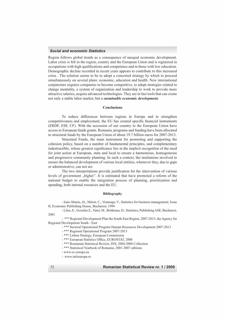
Romanian Statistical Review nr. 1 / 200952
Region follows global trends as a consequence of unequal economic development. Labor crisis is felt in the region, country and the European Union and is registered in occupations with high qualifi cations and competence and in those with low education. Demographic decline recorded in recent years appears to contribute to this increased crisis . The solution seems to be to adopt a concerted strategy by which to proceed simultaneously on several plans: economic, education and health. New international conjuncture requires companies to become competitive, to adopt strategies related to change mentality, a system of organization and leadership to work to provide more attractive salaries, acquire advanced technologies. They are in fact tools that can create not only a stable labor market, but a sustainable economic development.
Conclusions
To reduce differences between regions in Europe and to strengthen competitiveness and employment, the EU has created specifi c fi nancial instruments (ERDF, ESF, CF). With the accession of our country to the European Union have access to European funds grants. Romania, programs and funding have been allocated to structural funds by the European Union of about 19.7 billion euros for 2007-2013. Structural Funds, the main instrument for promoting and supporting the cohesion policy, based on a number of fundamental principles, and complementary indestructible, whose greatest signifi cance lies in the implicit recognition of the need for joint action at European, state and local to ensure a harmonious, homogeneous and progressive community planning. In such a context, the institutions involved to ensure the balanced development of various local entities, whenever they, due to gaps or administrative, can not act. The two interpretations provide justifi cation for the intervention of various levels of government „higher”. It is estimated that have promoted a reform of the national budget to enable the integration process of planning, prioritization and spending, both internal resources and the EU.
Bibliography
- Isaic-Maniu, Al., Mitrut, C., Voineagu, V., Statistics for business management, Issue II, Economic Publishing House, Bucharest, 1998 - Lilea, E., Goschin Z., Vatui, M., Boldeanu, D., Statistics, Publishing ASE, Bucharest, 2001 - *** Regional Development Plan the South-East Region, 2007-2013, the Agency for Regional Development South - East - *** Sectoral Operational Program Human Resources Development 2007-2013 - *** Regional Operational Program 2007-2013 - *** Lisbon Strategy, European Commission - *** European Statistics Offi ce, EUROSTAT, 2008 - *** Romanian Statistical Review, INS, 2004-2008 Collection - *** Statistical Yearbook of Romania, 2001-2007 editions - www.ec.europa.eu - www.infoeuropa.ro
Social and economic Statistics
Revista Română de Statistică nr. 1 / 2009 53
Rezultate distribuţionale ale Procesului Poisson- Dirichlet de două variabile Lector univ. dr. Mihail BUŞU Universitatea „Spiru Haret”
Abstract
În articol se prezintă rezultatele investigaţiei, proprietăţile şi aplicaţiile Distribuţiei Poisson- Dirichlet de două variabile. S-au stabilit notaţiile şi istoricul acestei distribuţii. Se demonstrează că procese cunoscute pentru serii probabilistice sunt cazuri particulare ale acestei distribuţii de două variabile. Distribuţia este maximală într-un anumit sens, care arată invarianţa faţă de permutaţii de aceeaşi lungime. Introducem Procesul Poisson- Dirichlet şi arătăm câteva dintre proprietăţile sale de bază. Se generalizează Procesul Dirichlet, care este un instrument des folosit de către statistica bayesiană de când aceasta s-a descoperit. Este analizată lungimea unui caz special al procesului Poisson- Dirichlet. Se descoperă o nouă clasă de densităţi ale simplexului şi discutăm calculele momentelor sale. În incheiere, se consideră variate realizări ale distribuţiei posterioare ale Procesului Poisson- Dirichlet. Cuvinte cheie: Distribuţie Poisson- Dirichlet, distribuţii posterioare, atomic, model, parametri, mostră, permutare, hipergeometric
* * * Studiul măsurilor probabilităţii aleatorii există încă din perioada lui Bayes, însă punerea sa în aplicare în statistica non- parametrică a lui Bayes s-a dovedit a fi greoaie şi destul de refractară până acum 25 de ani. Ferguson( 1973) propune o măsură a probabilităţii aleatorii, numită Procesul Dirichlet, pentru rezolvarea problemelor non- parametrice ale lui Bayes. Ferguson defi neşte Procesul Dirichlet recomandând distribuţia îmbinată a acestui proces care se aplică unei împărţiri măsurabile arbitrare a spaţiului măsurii. Se conferă o abordare constructivă a Procesului Dirichlet specifi când o secvenţă de puncte aleatorii( conform unei măsurători „ prior”) şi o secvenţă a probabilităţii aferentă, i.e., o secvenţă infi nită de variabile aleatorii non- negative care vor forma cu siguranţă una singură. Kingman( 1965) numeşte această secvenţă Distribuţia Poisson- Dirichlet. Existenţa a două reprezentări similare ale aceluiaşi proces aleatoriu nu este o coincidenţă. Pentru a explica legătura dintre ele, se prezintă câteva defi niţii:
Statistică matematică
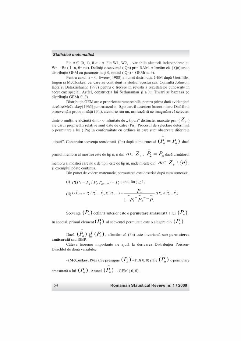
Romanian Statistical Review nr. 1 / 200954
Fie α Є [0, 1), θ > - α. Fie W1, W2,... variabile aleatorii independente cu Wn ~ Be ( 1- α, θ+ nα). Defi niţi o secvenţă ( Qn) prin RAM. Afi rmăm că ( Qn) are o distribuţie GEM cu parametri α şi θ, notată ( Qn) ~ GEM( α, θ). Pentru cazul α = 0, Ewens( 1988) a numit distribuţia GEM după Greiffi ths, Engen şi McCloskez, cei care au contribuit la studiul acestui caz. Consultă Johnson, Kotz şi Balakrishnan( 1997) pentru o trecere în revistă a rezultatelor cunoscute în acest caz special. Astfel, construcţia lui Sethuraman şi a lui Tiwari se bazează pe distribuţia GEM( 0, θ). Distribuţia GEM are o proprietate remarcabilă, pentru prima dată evidenţiată de către McCoskey( 1965) pentru cazul α = 0, pe care îl descriem în continuare. Dată fi ind o secvenţă a probabilităţii ( Pn), aleatorie sau nu, urmează să ne imaginăm că selectaţi
dintr-o mulţime alcăuită dintr- o infi nitate de „ tipuri” distincte, marcate prin ( +Z ) ale cărui proprietăţi relative sunt date de către (Pn). Procesul de selectare determină o permutare a lui ( Pn) în conformitate cu ordinea în care sunt observate diferitele
„tipuri”. Construim secvenţa reordonată (Pn) după cum urmează )(~
nn PP = dacă
primul membru al mostrei este de tip n, n din +∈Zn ; mPP =~
2 dacă următorul
membru al mostrei care nu e de tip n este de tip m, unde m este din }{\ nZm +∈ ; şi exemplul poate continua. Din punct de vedere matematic, permutarea este descrisă după cum urmează:
(i) nn PPPPPP == ,....),/( 211
~; and, for j > 1,
(ii) ).,...(~
...~~
,....),,,..../(~~
1
21
21
~~
11
~
1jn
j
njnj PPPIPPPPPPP
PPP
P ≠−−
==
−+
Secvenţa )(~
nP defi nită anterior este o permutare amăsurată a lui )( nP .
În special, primul element )(~
1P al secvenţei permutate este o alegere din )( nP .
Dacă )(~
nP d )( nP , afi rmăm că (Pn) este invariantă sub permuterea amăsurată sau ISBP. Câteva teoreme importante ne ajută la derivarea Distribuţiei Poisson- Dirichlet de două variabile.
- (McCoskey, 1965). Se presupue )( nP ~ PD( 0, θ) şi fi e )(~
nP o permutare
amăsurată a lui )( nP . Atunci )(~
nP ~ GEM ( 0, θ).
Statistică matematică
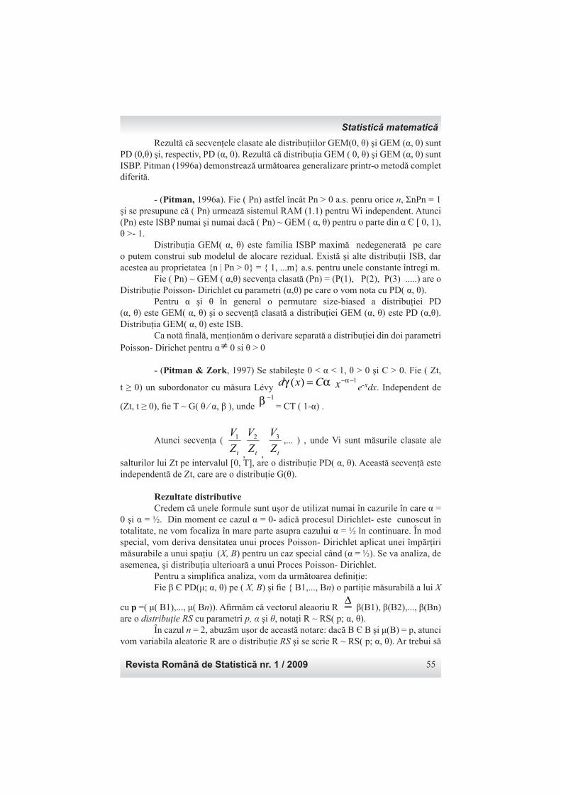
Revista Română de Statistică nr. 1 / 2009 55
Rezultă că secvenţele clasate ale distribuţiilor GEM(0, θ) şi GEM (α, 0) sunt PD (0,θ) şi, respectiv, PD (α, 0). Rezultă că distribuţia GEM ( 0, θ) şi GEM (α, 0) sunt ISBP. Pitman (1996a) demonstrează următoarea generalizare printr-o metodă complet diferită.
- (Pitman, 1996a). Fie ( Pn) astfel încât Pn > 0 a.s. penru orice n, ΣnPn = 1 şi se presupune că ( Pn) urmează sistemul RAM (1.1) pentru Wi independent. Atunci (Pn) este ISBP numai şi numai dacă ( Pn) ~ GEM ( α, θ) pentru o parte din α Є [ 0, 1), θ >- 1. Distribuţia GEM( α, θ) este familia ISBP maximă nedegenerată pe care o putem construi sub modelul de alocare rezidual. Există şi alte distribuţii ISB, dar acestea au proprietatea {n | Pn > 0} = { 1, ...m} a.s. pentru unele constante întregi m. Fie ( Pn) ~ GEM ( α,θ) secvenţa clasată (Pn) = (P(1), P(2), P(3) .....) are o Distribuţie Poisson- Dirichlet cu parametri (α,θ) pe care o vom nota cu PD( α, θ). Pentru α şi θ în general o permutare size-biased a distribuţiei PD (α, θ) este GEM( α, θ) şi o secvenţă clasată a distribuţiei GEM (α, θ) este PD (α,θ). Distribuţia GEM( α, θ) este ISB. Ca notă fi nală, menţionăm o derivare separată a distribuţiei din doi parametri Poisson- Dirichet pentru α≠ 0 si θ > 0
- (Pitman & Zork, 1997) Se stabileşte 0 < α < 1, θ > 0 şi C > 0. Fie ( Zt,
t ≥ 0) un subordonator cu măsura Lévy αγ Cxd =)( 1−−αx e-xdx. Independent de
(Zt, t ≥ 0), fi e T ~ G( θ ⁄ α, β ), unde 1−β = CT ( 1-α) .
Atunci secvenţa ( tZ
V1
, tZ
V2
, tZ
V3 ,... ) , unde Vi sunt măsurile clasate ale
salturilor lui Zt pe intervalul [0, T], are o distribuţie PD( α, θ). Această secvenţă este independentă de Zt, care are o distribuţie G(θ).
Rezultate distributive Credem că unele formule sunt uşor de utilizat numai în cazurile în care α = 0 şi α = ½. Din moment ce cazul α = 0- adică procesul Dirichlet- este cunoscut în totalitate, ne vom focaliza în mare parte asupra cazului α = ½ în continuare. În mod special, vom deriva densitatea unui proces Poisson- Dirichlet aplicat unei împărţiri măsurabile a unui spaţiu (X, B) pentru un caz special când (α = ½). Se va analiza, de asemenea, şi distribuţia ulterioară a unui Proces Poisson- Dirichlet. Pentru a simplifi ca analiza, vom da următoarea defi niţie: Fie β Є PD(μ; α, θ) pe ( X, B) şi fi e { B1,..., Bn) o partiţie măsurabilă a lui X
cu p =( μ( B1),..., μ( Bn)). Afi rmăm că vectorul aleaoriu R∆
β(B1), β(B2),..., β(Bn) are o distribuţie RS cu parametri p, α şi θ, notaţi R ~ RS( p; α, θ). În cazul n = 2, abuzăm uşor de această notare: dacă B Є B şi μ(B) = p, atunci vom variabila aleatorie R are o distribuţie RS şi se scrie R ~ RS( p; α, θ). Ar trebui să
Statistică matematică
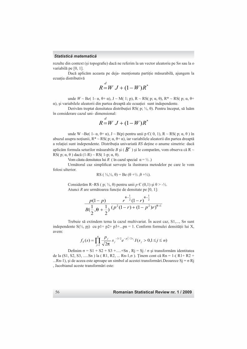
Romanian Statistical Review nr. 1 / 200956
rezulte din context (şi topografi e) dacă ne referim la un vector aleatoriu pe Sn sau la o variabilă pe [0, 1]. Dacă aplicăm aceasta pe deja- menţionata partiţie măsurabilă, ajungem la ecuaţia distributivă
*)1( RWJWRd
−+=
unde W ~ Be( 1- α, θ+ α), J ~ M( 1; p), R ~ RS( p; α, θ), R* ~ RS( p; α, θ+ α), şi variabilele aleatorii din partea dreaptă ale ecuaţiei sunt independente. Derivăm treptat densitatea distribuţiei RS( p; ½, θ). Pentru început, să luăm în considerare cazul uni- dimensional:
*)1( RWJWRd
−+=
unde W ~Be( 1- α, θ+ α), J ~ B(p) pentru unii p Є( 0, 1), R ~ RS( p; α, θ ) în abuzul asupra noţiunii, R* ~ RS( p; α, θ+ α), iar variabilele aleatorii din partea dreaptă a relaţiei sunt independente. Distribuţia univariată RS deţine o anume simetrie: dacă
aplicăm formula seturilor măsurabile B şi ( cB ) şi le comparăm, vom observa că R ~ RS( p; α, θ ) dacă (1-R) ~ RS( 1-p; α, θ). Vom căuta densitatea lui R ( în cazul special α = ½ .) Următorul caz simplifi cat serveşte la ilustrarea metodelor pe care le vom folosi ulterior.
RS ( ½,½, θ) = Be (θ +½ ,θ +½).
Considerăm R~RS ( p; ½, θ) pentru unii p Є (0,1) şi θ > -½. Atunci R are următoarea funcţie de densitate pe [0, 1]:
122
2
1
2
1
))1()1((
)1(
)2
1,
2
1(
)1(+
−−
−+−−
+
−θ
θθ
θrprp
rr
B
pp
Trebuie să extindem tema la cazul multivariat. În acest caz, S1,..., Sn sunt independente S(½, pj) cu p1+ p2+ p3+...pn = 1. Conform formulei densităţii lui X, avem:
)1,0(2
)(1
2/2/3 2
njsIesp
sfn
jj
sp
jj
Sjj ≤≤>=∏
=
−−
π
Defi nim σ = S1 + S2 + S3 +.....+Sn , Rj = Sj / σ şi transformăm identitatea de la (S1, S2, S3, .....Sn ) la ( R1, R2, ... Rn-1,σ ). Ţinem cont că Rn = 1-( R1+ R2 + ...Rn-1), şi de aceea este aproape un simbol al acestei transformări.Deoarece Sj = σ Rj , Jacobianul aceste transformări este:
Statistică matematică
Revista Română de Statistică nr. 1 / 2009 57
1
1
2
1
11
1
...
...00
........................
0...0
0...0
),,...,(
),...( −
−
−
=
−−
=∂∂ n
n
n
n
n
R
R
R
R
RR
SSσ
σσ
σ
σ
σ
σ
şi atunci
∏=
−−− ×=n
j
nrp
jj
Rjjer
prf
1
12/2/3,
2
)(2
),( σσπ
σσ
σ
}.)/(2
1exp{...
)2(
...
1
22
22/32/3
12/1 ∑
=
+−−− −=
n
jjj
n
nnn rprr
pp
σσ
π
Integrând dupa σ obţinem,
)())/(
2)
2(...
)2(
...)(
1
2/2
2/2/32/3
12/1
nn njj
n
nnn
R SrIrp
nrr
pprf ∈Γ=
∑−−
π
)(
)...(
...)2
(...
2/2
1
21
2/32/31
2/
1
nn
n
n
nn
n
SrI
r
p
r
p
rrn
pp∈
++
Γ=
−−
π
Simplifi cat, vom nota cu X pe R*. Condiţionând R pe J = ej,
XWeWeJR j
d
j )1( }/{ −+==
Notăm cu Y această condiţională pe R. Deoarece X si W sunt independente,
),(
)1(),(
2/12/1
, xfww
wxf XWXπ
−− −=
apoi substituind: yi = ωij + (1-ω) xi, obţinem:
⇒−==∂∂ −
−
− n
n
n wyy
xx 1
11
11 )1(...),...(
),...(
Statistică matematică
Romanian Statistical Review nr. 1 / 200958
.)1( )
1,...,
1,...,
1(
)1(),( 11
2/12/1
,nnj
XWY ww
y
w
wy
w
yf
wwwyf −
−−
−−−
−
−−
=π
Integrând după ω obţinem:
. )1
,...,1
,...,1
()1(
)( 12/12/1
0wd
w
y
w
wy
w
yf
wwyf nj
X
y
Y
j
−−
−
−−
=−−
∫ π Formăm distribuţia condiţională a lui R reducând toate valorile posibile ale lui J, şi obţinem:
. )1
(
)1()(
2/12/1
01
wdw
ewrf
wwprf j
X
nrn
jjR
j
−
−−=
−−
=∫∑
π
Fie R~ RS (p,½, θ) pentru unii p Є Sn si θ > -½. Atunci densitatea lui R este
).(
)...(
...
)2
1(
)2
(...)(
22
1
21
2/32/31
2
1
1
nn
n
n
nn
n
R SrI
r
p
r
p
rrn
pprf ∈
+++Γ
+Γ=
+
−−
−θ
θπ
θ
Formulele momentelor pentru funcţia densităţii
Metoda utilizată pentru calcularea momentelor lui R = β( B) trebuie folosită cu foarte mare grijă. Metoda nu se aplică pentru momente mai mari de 3 pentru că apar termeni care nu sunt acoperiţi de Lema 1. În cazul special al lui α=½, cunoaştem densitatea lui R din lema precedentă şi putem spera să obţinem astfel de momente generale în acest fel.
∫ ∫ +
−−+
−+−−
+
−==
1
0
1
0122
2/12/1
])1()1([
)1(
)2
1,
2
1(
)1( )( xd
xpxp
xx
B
ppxdxfxRE
n
Rnn
θ
θθ
θ
Funcţia hipergeometrică Gauss H( a, b, c, z) este dată de expresia integrală
∫ −−−− −−−
=1
0
11 ) 1()1(),(
1),,,( tdzttt
bcbBzcbaH abcb
Statistică matematică
Revista Română de Statistică nr. 1 / 2009 59
Rezultă:
∫ +−−−+
+
−−
+
−=
1
0
)1(2/12/1
12
) 1()1(
2
1,
2
11
xdxzxxBp
pRE nn θθθ
θ θ
),,12,
2
1,1(
2
1,
2
12
1,
2
1)1(
12
znnH
Bp
nBp
+++++
+
+++−=
+
θθθ
θ
θθ
θ
unde z = (2p-1) / p² . Catalogăm unele din cunoscutele proprietăţi ale funcţiei hipergeometrie Gauss folosită în cele ce urmează: Fie H( a, b, c, z) defi nită.
∑=
−−
−
−
−=−
∈
−−−=
−−−−−=
−+=
=+−−+
−−−−−=−−−−
−−=
m
k
k
k
kk
bac
/
a
,z(c)
(b)
k
m)(m,b,c,z)(H
N,m(v)For
b,c,z).a,cH(cz )(,c,z)(i v)H(a,b
).z
,c,b,aH (z )(H(a,b,c,z)
,thenbac(iii)I f
,z)cb)z H(a,b,a) (c( c
,z))z]H(a,b,cbac(c[c,z))H(a,b,c) (z(ii)c(c
).z
zb,c,H(a,cz )(,z)(i)H(a,b,c
0
21
1
1
2
1112121
2
1
01
1211111
1
unde (x)n = x(x+1)(x+2)...(x+n-1) = Γ(x+n) / Γ(x)
Aplicând Lema 3 (i) , după mici calcule, obţinem:
).)1(
21,12,
2
1,1(
2
1,
2
1)1(
2
1,
2
1
2
12 p
pnH
Bp
nBp
RE n
−−
++++
+−
+++=
+
θθθ
θ
θθ
θ
Statistică matematică
Romanian Statistical Review nr. 1 / 200960
Rezultă
)1()1(
21)
2
1( )1(
)(])1(
21)
2
522(12[ )2(
)1()1(
)12( )2(0
2
2
2
2
+−−
−+−+
+−−
−+−−++
+−−
−++−=
nhp
pnn
nhp
pnnn
nhp
pnn
θθ
θθθ
θθ
Pentru simplifi care notăm mn = ERn. Ştim că pentru n>1 avem:
)(
2
1,
2
1)1(
2
1,
2
1
121 nh
Bp
nBpmn
+−
+−+=
+−
θ
θθ
θ
şi
).1(
2
1,
2
1)1(
2
1,
2
3
122 −
+−
+−+=
+− nh
Bp
nBp
mn
θ
θθ
θ
Se introduc aceste valori şi calculăm mn în funcţie de mn-1 şi mn-2 Se obţine următorul rezultat: Fie R~ RS (p,½, θ) pentru θ > -½ si p≠ ½ si fi e mn = ERn.
)12)(1(2
))12(2)24(63()223(
,2,,
),0(1
122
22
1
0
−−+−++−+−+−−
=
≥=
≠=
−−
pn
mppnppmpnm
nforandpm
pm
nnn
θ
θθ
Notă: Dacă p = 0, 1, unele din expresiile intermediare care duc la acest rezultat sunt lipsite de importanţă; totuşi, formula fi nală rămâne valabilă. De exemplu, dacă p = 1, atunci toate momentele lui R sunt egale cu 1, şi Lema 4 confi rmă faptul că:
.1)12)(1(2
))121(22463()223(≡
−−+++−+−+−+−−
=n
nnmn
θ
θθ
Problemele apar când p=½. Este curios că mn se dovedeşte a fi un polinominal de grad n în p, astfel încât termenul (2p- 1) din numitorul Lemei 4. trebuie să se anuleze cu termenii menţionaţi. Acest aspect nu se poate observa în cadrul formulei
Statistică matematică
Revista Română de Statistică nr. 1 / 2009 61
recursive. Pentru p=½, trebuie să folosim în schimb unul din rezultatele recente; şi anume R ~ Be(θ+½, θ+½) dată de Lema 1. Oferim o formulă închisă pentru momentele lui R. Să presupunem că R~ RS (p,½, θ).
.)2
1(
)12(
)(1
2
2,
2
12
1,
2
1
1
0∑−
=
−−++
−
++
++
+++=
n
k
knk
k
kn ppn
n
k
n
nnB
nB
REθ
θθ
θθ
Densitatea distribuţiei posterioare
În cadrul aplicaţiei statisticii lui Bayes, presupunem o distribuţie „ prioritară” pentru parametrii din modelul prezentat. Înainte de a observa datele, ştim cum ar trebui distribuiţi parametrii (consideraţi variabile aleatorii). Această distribuţie prioritară se noatează prin π(.) După ce am observat datele, ne-am schimbat părerea despre distribuţia parametrilor şi am format distribuţia „prioritară”. Distribuţia posterioară, dată fi ind X = x, este notată π(. /x). Pentru a exemplifi ca această metodă, calculăm o distribuţie posterioară care ocupă un loc dominant: Fie W = ( W1 ,W2, W3, ....Wn ) un vector şi considerăm o distribuţie Diriclet W ~ D(α1, α2, ... αn ). Condiţional pe W, fi e X~ M(1;W); astfel încât
.1.,.)/( njsaWWeXP jj ≤≤== Calculăm distribuţia posterioară a lui W condiţionată de X după cum urmează:
⇒=
==−−
−−
jn
jn
w
www
wWeXPww
n
n
....
)/(....11
1
111
1
1
αα
ααα
),,...,(~}/{
)()(
1 ααj
n
j
j DeXW =
unde )( j
iα= iα
+ ij∂ . Rezultă că distribuţia posterioară a lui W este de asemenea o distribuţie Dirichlet, dar cu un parametru ajustat.
Statistică matematică
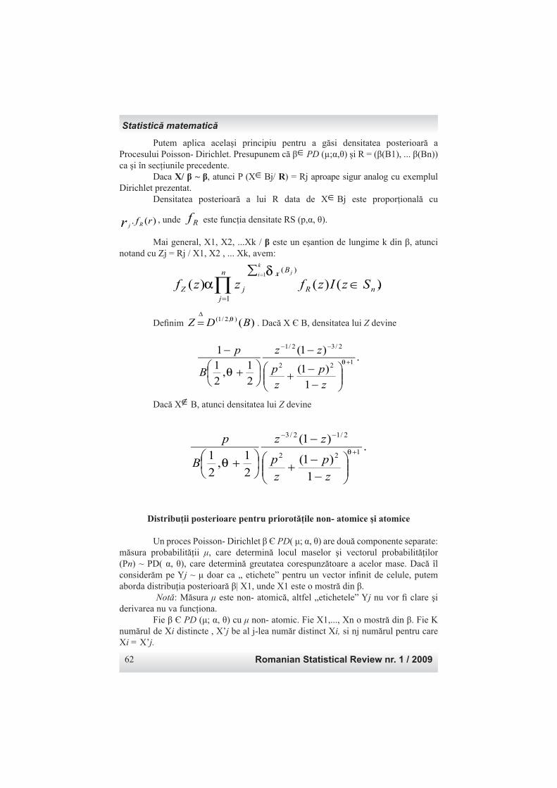
Romanian Statistical Review nr. 1 / 200962
Putem aplica acelaşi principiu pentru a găsi densitatea posterioară a Procesului Poisson- Dirichlet. Presupunem că β∈PD (µ;α,θ) şi R = (β(B1), ... β(Bn)) ca şi în secţiunile precedente. Daca X/ β ~ β, atunci P (X∈Bj/ R) = Rj aproape sigur analog cu exemplul Dirichlet prezentat. Densitatea posterioară a lui R data de X∈Bj este proporţională cu
)(. rfRjr , unde Rf este funcţia densitate RS (p,α, θ).
Mai general, X1, X2, ...Xk / β este un eşantion de lungime k din β, atunci notand cu Zj = Rj / X1, X2 , ... Xk, avem:
).()()(1
)(
1nR
Bn
jjZ SzIzfzzf
k
i jXi
∈∑ =
∏=
δα
Defi nim )(),2/1( BDZ θ∆
= . Dacă X Є B, densitatea lui Z devine
.
1
)1(
)1(
2
1,
2
11
122
2/32/1
+
−−
−−
+
−
+
−θ
θz
p
z
p
zz
B
p
Dacă X∉B, atunci densitatea lui Z devine
.
1
)1(
)1(
2
1,
2
1 122
2/12/3
+
−−
−−
+
−
+θ
θz
p
z
p
zz
B
p
Distribuţii posterioare pentru priorotăţile non- atomice şi atomice
Un proces Poisson- Dirichlet β Є PD( μ; α, θ) are două componente separate: măsura probabilităţii μ, care determină locul maselor şi vectorul probabilităţilor (Pn) ~ PD( α, θ), care determină greutatea corespunzătoare a acelor mase. Dacă îl considerăm pe Yj ~ μ doar ca „ etichete” pentru un vector infi nit de celule, putem aborda distribuţia posterioară β| X1, unde X1 este o mostră din β. Notă: Măsura μ este non- atomică, altfel „etichetele” Yj nu vor fi clare şi derivarea nu va funcţiona. Fie β Є PD (μ; α, θ) cu μ non- atomic. Fie X1,..., Xn o mostră din β. Fie K numărul de Xi distincte , X’j be al j-lea număr distinct Xi, si nj numărul pentru care Xi = X’j.
Statistică matematică
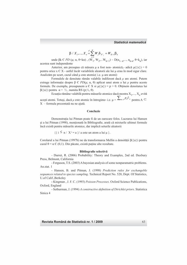
Revista Română de Statistică nr. 1 / 2009 63
kK
K
jXj
d
n WWXXj
βδβ 11
'1,...,/ +=
+=∑ unde βk Є PD (μ; α, θ+kα) , (W1, W2,...Wk+1) ~ D(n1- α,..., nk-α, θ+kα), iar acestea sunt independente Anterior, am presupus că măsura μ a fost non- atomică,- adică μ({x}) = 0 pentru orice x Є X - astfel încât variabilele aleatorii ale lui μ erau în mod sigur clare. Analizăm pe scurt, cazul când μ este atomic( i.e. μ are atomi) Formulele de densitate rămân valabile indiferent dacă μ are atomi. Putem extrage informaţie despre β Є PD(μ; α, θ) aplicat unui atom a lui μ pentru aceste formule. De exemplu, presupunem a Є X si μ({a}) = p > 0. Obţinem densitatea lui β({a}) pentru α = ½ , numita RS (p;½, θ). Ecuaţia rămâne valabilă pentru măsurile atomice dacă mostra X1,..., Xn evită
aceşti atomi. Totuşi, dacă μ este atomic în întregime- i.e. μ = aAa ap ∂∑ ∈ pentru A ⊂ X – formula prezentată nu ne ajută.
Concluzie
Demonstraţia lui Pitman poate fi de un oarecare folos. Lucrarea lui Hansen şi a lui Pitman (1998), menţionată în Bibliografi e, arată că mixturile ultimei formule încă există pentru măsurile atomice, dar implică seturile aleatorii
{{ i ≤ n / X i = a }/ a este un atom a lui μ }.
Corolarul a lui Pitman (1997b) ne da transformarea Mellin a densităţii β({a}) pentru cazul θ = α Є (0,1). Din păcate, există puţine alte rezultate.
Bibliografi e selectivă - Durret, R. (2006) Probability: Theory and Examples, 2nd ed. Duxbury Press, Belmont, California - Ferguson, T.S. (2003) A bayesian analysis of some nonparamatric problems. An.stat. 1 - Hansen, B. and Pitman, J. (1998) Prediction rules for exchangeble sequances related to species sampling. Technical Report No. 520, Dept. Of Statistics, U.of Calif.,Berkeley - Kingman , J. F. C. (1993) Poisson Processes. Oxford Science Publications, Oxford, England - Sethurman, J. (1994) A constructive defi nition of Dirichlet priors. Statistica Sinica 4
Statistică matematică
Romanian Statistical Review nr. 1 / 200964
DISTRIBUTIONAL RESULTS OF THE TWO PARAMETER POISSON- DIRICHLET
DISTRIBUTION
Ph.D. Lecturer Mihail BUŞU „Spiru Haret” University
ABSTRACT In this article are presented the results of the investigations of the properties and applications of the two parameter Poisson- Dirichlet Distribution. It were established notations and it was described the background history of this distribution. It has been shown that certain previously-known distributions for probability sequences are marginal cases of this two-parameter distribution. This distribution is in some sense maximal among those distributions which exhibit invariance under size-biased permutation. We then introduce the related Poisson- Dirichlet process and show some of its more basic properties. This generalizes the Dirichlet process, which has been a popular tool for Bayesian statisticians since discovery. In particular, we investigate at length a new special case of the Poisson- Dirichlet process. Therein, we uncover a new class of densities on the simplex and discuss computation of its moments. We also consider various realizations of the posterior distribution of the Poisson- Dirichlet process. Key-words: distribution, Poisson- Dirichlet, posterior, model, parameters, sample, permutations, hypergeometric
* * * While the study of the random probability measures has been around since the time of Bayes, its application to Bayesian non-parametric statistics proved cumbersome and fairly intractable until about twenty-fi ve years ago. Ferguson (1973) proposes a random probability measure, called a Dirichlet process, for treating Bayesian non-parametric problems. Ferguson defi nes the Dirichlet process by prescribing the joint distribution of this process applied to an arbitrary measurable partition of the measure space. This same article gives a constructive approach to the Dirichlet process by specifying a sequence of random points (according to some “prior” measure) and a corresponding probability sequence; i.e., an infi nite sequence of non-negative random variables which sums to one almost surely. Kingman(1975) terms this probability sequence the Poisson- Dirichlet distribution. The existence of two similar-looking representations of the same random process is no coincidence. To begin to explain their connection, we present some defi nitions. Let α Є [0, 1), θ > - α. Let W1, W2,... be independent random variables with Wn ~ Be ( 1- α, θ+ nα). Defi ne a sequence (Qn ) by the RAM as above. Then we say (Qn) has a GEM distribution with parameters α and θ, denoted (Qn) ~ GEM(α, θ). For the α = 0 case, Ewens (1988) named above distribution GEM for Griffi ths, Engen and McCloskey, who contributed to the study of this case. See Johnson, Kotz, and Balakrishnan (1997) for a survey of known results in this special case. Sethuraman
Mathematical Statistics
Revista Română de Statistică nr. 1 / 2009 65
and Tiwari’s construction above in thus based upon the GEM(0, θ) distribution. The GEM distribution has a remarkable property, fi rst known by McCloseky (1965) for the α = 0 case, which we describe here. Given a probability sequence (Pn), random or not, imagine sampling from a population of infi nitely- many distinct ‚”types”, labeled by Z+, whose relative proportions are given by (Pn). The act of sampling induces a permutation of (Pn) according to the order in which the different „types” are observed.
In words, we construct the reordered sequence )(~
nP as follows nPP =1
~
if the
fi rst member of the sample is of type n, +∈Zn ; mPP =~
2 if the next member of
the sample not of type n is of type m, }{\ nZm +∈ ; and so on.Mathematically, the permutation is described as follows:
(i) nn PPPPPP == ,....),/( 211
~
; and, for j > 1,
(ii)
).,...(~
...~~
,....),,,..../(~~
1
21
21
~~
11
~
1jn
j
njnj PPPIPPPPPPP
PPP
P ≠−−
==
−+
The sequence )(~
nP defi ned above is a size-biased permutation of )( nP .
In particular, the fi rst element )(~
1P of the permuted sequence is a size-pick from
)( nP .
If )(~
nP d )( nP , we say that )( nP is invariant under sized bised permutation, or ISBP. A few important theorems help us to derive the two parameter Poisson-Dirichlet distribution.
(McCloskey, 1965) Suppose )( nP ~PD(0, θ) and let )(~
nP be a size-
biased permutation of )( nP . Then )(~
nP ~GEM( 0, θ).
It follows from these results that the ranked sequences of the GEM (0, θ) and GEM(α, 0) distributions are are PD(0, θ) and PD(α, 0), respectively. Moreover, it follows that the GEM (0, θ) and GEM(α, 0) distributions are ISBP.
Let )( nP be such that nP >0 a.s for all n, 1=∑ nnP , and suppose
Mathematical Statistics
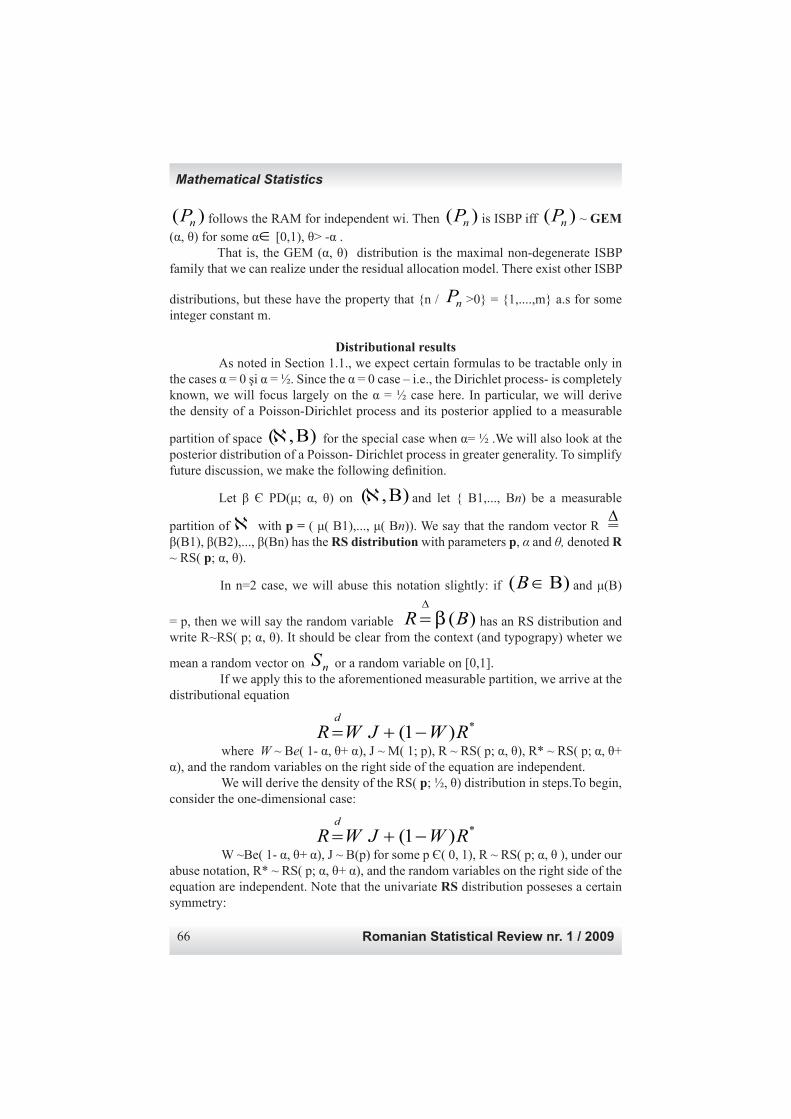
Romanian Statistical Review nr. 1 / 200966
)( nP follows the RAM for independent wi. Then )( nP is ISBP iff )( nP ~ GEM (α, θ) for some α∈ [0,1), θ> -α . That is, the GEM (α, θ) distribution is the maximal non-degenerate ISBP family that we can realize under the residual allocation model. There exist other ISBP
distributions, but these have the property that {n / nP >0} = {1,....,m} a.s for some integer constant m.
Distributional results As noted in Section 1.1., we expect certain formulas to be tractable only in the cases α = 0 şi α = ½. Since the α = 0 case – i.e., the Dirichlet process- is completely known, we will focus largely on the α = ½ case here. In particular, we will derive the density of a Poisson-Dirichlet process and its posterior applied to a measurable
partition of space ),( Βℵ for the special case when α= ½ .We will also look at the posterior distribution of a Poisson- Dirichlet process in greater generality. To simplify future discussion, we make the following defi nition.
Let β Є PD(μ; α, θ) on ),( Βℵ and let { B1,..., Bn) be a measurable
partition of ℵ with p = ( μ( B1),..., μ( Bn)). We say that the random vector R∆
β(B1), β(B2),..., β(Bn) has the RS distribution with parameters p, α and θ, denoted R ~ RS( p; α, θ).
In n=2 case, we will abuse this notation slightly: if )( Β∈B and μ(B)
= p, then we will say the random variable )(BR β∆
= has an RS distribution and write R~RS( p; α, θ). It should be clear from the context (and typograpy) wheter we
mean a random vector on nS or a random variable on [0,1]. If we apply this to the aforementioned measurable partition, we arrive at the distributional equation
*)1( RWJWRd
−+= where W ~ Be( 1- α, θ+ α), J ~ M( 1; p), R ~ RS( p; α, θ), R* ~ RS( p; α, θ+ α), and the random variables on the right side of the equation are independent. We will derive the density of the RS( p; ½, θ) distribution in steps.To begin, consider the one-dimensional case:
*)1( RWJWRd
−+= W ~Be( 1- α, θ+ α), J ~ B(p) for some p Є( 0, 1), R ~ RS( p; α, θ ), under our abuse notation, R* ~ RS( p; α, θ+ α), and the random variables on the right side of the equation are independent. Note that the univariate RS distribution posseses a certain symmetry:
Mathematical Statistics
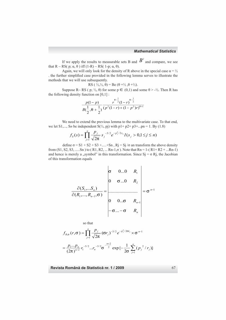
Revista Română de Statistică nr. 1 / 2009 67
If we apply the results to measurable sets B and cB and compare, we see
that R ~ RS( p; α, θ ) iff (1-R) ~ RS( 1-p; α, θ). Again, we will only look for the density of R above in the special case α = ½ . the further simplifi ed case provided in the following lemma serves to illustrate the methods that we will use subsequently.
RS ( ½,½, θ) = Be (θ +½ ,θ +½). Suppose R~ RS ( p; ½, θ) for some p ∈ (0,1) and some θ > -½. Then R has the following density function on [0,1] :
122
2
1
2
1
))1()1((
)1(
)2
1,
2
1(
)1(+
−−
−+−−
+
−θ
θθ
θrprp
rr
B
pp
We need to extend the previous lemma to the multivariate case. To that end, we let S1,..., Sn be independent S(½, pj) with p1+ p2+ p3+...pn = 1. By (1.8)
)1,0(2
)(1
2/2/3 2
njsIesp
sfn
jj
sp
jj
Sjj ≤≤>=∏
=
−−
π
defi ne σ = S1 + S2 + S3 +.....+Sn , Rj = Sj /σ an transform the above density from (S1, S2, S3, .....Sn ) to ( R1, R2, ... Rn-1,σ ). Note that Rn = 1-( R1+ R2 + ...Rn-1) and hence is merely a „symbol” in this transformation. Since Sj = σ Rj, the Jacobian of this transformation equals
1
1
2
1
11
1
...
...00
........................
0...0
0...0
),,...,(
),...( −
−
−
=
−−
=∂∂ n
n
n
n
n
R
R
R
R
RR
SSσ
σσ
σ
σ
σ
σ
so that
∏=
−−− ×=n
j
nrp
jj
Rjjer
prf
1
12/2/3,
2
)(2
),( σσπ
σσ
σ
}.)/(
2
1exp{...
)2(
...
1
22
22/32/3
12/1 ∑
=
+−−− −=
n
jjj
n
nnn rprr
pp
σσ
π
Mathematical Statistics
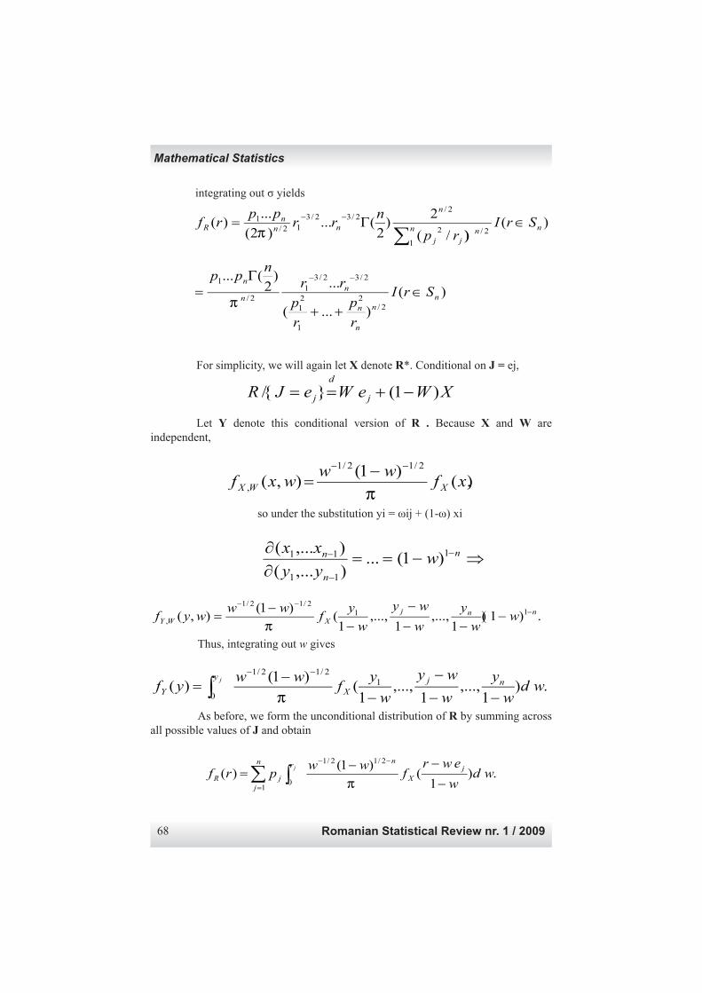
Romanian Statistical Review nr. 1 / 200968
integrating out σ yields
)())/(
2)
2(...
)2(
...)(
1
2/2
2/2/32/3
12/1
nn njj
n
nnn
R SrIrp
nrr
pprf ∈Γ=
∑−−
π
)(
)...(
...)2
(...
2/2
1
21
2/32/31
2/
1
nn
n
n
nn
n
SrI
r
p
r
p
rrn
pp∈
++
Γ=
−−
π
For simplicity, we will again let X denote R*. Conditional on J = ej,
XWeWeJR j
d
j )1( }/{ −+==
Let Y denote this conditional version of R . Because X and W are independent,
),()1(
),(2/12/1
, xfww
wxf XWXπ
−− −=
so under the substitution yi = ωij + (1-ω) xi
⇒−==∂∂ −
−
− n
n
n wyy
xx 1
11
11 )1(...),...(
),...(
.)1)(1
,...,1
,...,1
()1(
),( 112/12/1
,nnj
XWY ww
y
w
wy
w
yf
wwwyf −
−−
−−−
−
−−
=π
Thus, integrating out w gives
. )1
,...,1
,...,1
()1(
)( 12/12/1
0wd
w
y
w
wy
w
yf
wwyf nj
X
y
Y
j
−−
−
−−
=−−
∫ π As before, we form the unconditional distribution of R by summing across all possible values of J and obtain
. )1
(
)1()(
2/12/1
01
wdw
ewrf
wwprf j
X
nrn
jjR
j
−
−−=
−−
=∫∑
π
Mathematical Statistics
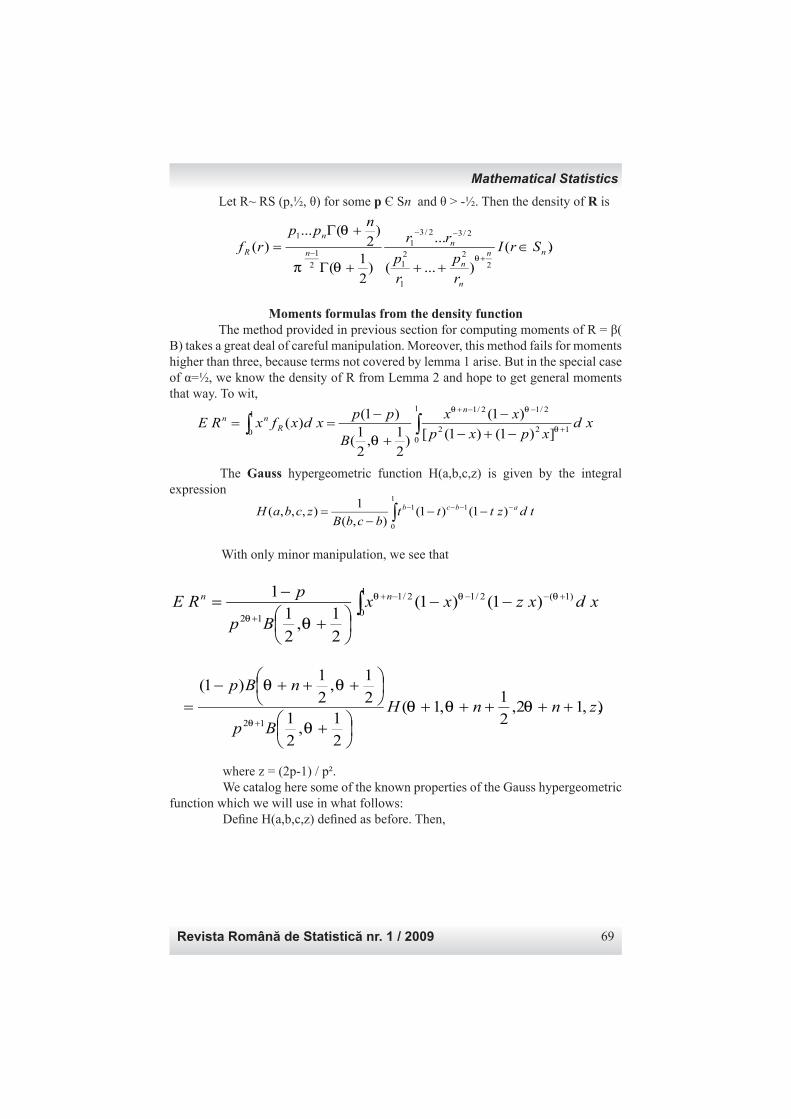
Revista Română de Statistică nr. 1 / 2009 69
Let R~ RS (p,½, θ) for some p Є Sn and θ > -½. Then the density of R is
).(
)...(
...
)2
1(
)2
(...)(
22
1
21
2/32/31
2
1
1
nn
n
n
nn
n
R SrI
r
p
r
p
rrn
pprf ∈
+++Γ
+Γ=
+
−−
−θ
θπ
θ
Moments formulas from the density function The method provided in previous section for computing moments of R = β( B) takes a great deal of careful manipulation. Moreover, this method fails for moments higher than three, because terms not covered by lemma 1 arise. But in the special case of α=½, we know the density of R from Lemma 2 and hope to get general moments that way. To wit,
∫ ∫ +
−−+
−+−−
+
−==
1
0
1
0122
2/12/1
])1()1([
)1(
)2
1,
2
1(
)1( )( xd
xpxp
xx
B
ppxdxfxRE
n
Rnn
θ
θθ
θ
The Gauss hypergeometric function H(a,b,c,z) is given by the integral expression
∫ −−−− −−−
=1
0
11 ) 1()1(),(
1),,,( tdzttt
bcbBzcbaH abcb
With only minor manipulation, we see that
∫ +−−−+
+
−−
+
−=
1
0
)1(2/12/1
12
) 1()1(
2
1,
2
11
xdxzxxBp
pRE nn θθθ
θ θ
),,12,
2
1,1(
2
1,
2
12
1,
2
1)1(
12
znnH
Bp
nBp
+++++
+
+++−=
+
θθθ
θ
θθ
θ
where z = (2p-1) / p². We catalog here some of the known properties of the Gauss hypergeometric function which we will use in what follows: Defi ne H(a,b,c,z) defi ned as before. Then,
Mathematical Statistics
Romanian Statistical Review nr. 1 / 200970
∑=
−−
−
−
−=−
∈
−−−=
−−−−−=
−+=
=+−−+
−−−−−=−−−−
−−=
m
k
k
k
kk
bac
/
a
,z(c)
(b)
k
m)(m,b,c,z)(H
N,m(v)For
b,c,z).a,cH(cz )(,c,z)(i v)H(a,b
).z
,c,b,aH (z )(H(a,b,c,z)
,thenbac(iii)I f
,z)cb)z H(a,b,a) (c( c
,z))z]H(a,b,cbac(c[c,z))H(a,b,c) (z(ii)c(c
).z
zb,c,H(a,cz )(,z)(i)H(a,b,c
0
21
1
1
2
1112121
2
1
01
1211111
1
where (x)n = x(x+1)(x+2)...(x+n-1) = Γ(x+n) / Γ(x) Applying lema 3(i), after short computations, we get:
).)1(
21,12,
2
1,1(
2
1,
2
1)1(
2
1,
2
1
2
12 p
pnH
Bp
nBp
RE n
−−
++++
+−
+++=
+
θθθ
θ
θθ
θ
and then
)1()1(
21)
2
1( )1(
)(])1(
21)
2
522(12[ )2(
)1()1(
)12( )2(0
2
2
2
2
+−−
−+−+
+−−
−+−−++
+−−
−++−=
nhp
pnn
nhp
pnnn
nhp
pnn
θθ
θθθ
θθ
For simplicity, let mn = ERn. Then we know from (3.18) that, for n > 2,
)(
2
1,
2
1)1(
2
1,
2
1
121 nh
Bp
nBpmn
+−
+−+=
+−
θ
θθ
θ
and
).1(
2
1,
2
1)1(
2
1,
2
3
122 −
+−
+−+=
+− nh
Bp
nBp
mn
θ
θθ
θ
Mathematical Statistics
Revista Română de Statistică nr. 1 / 2009 71
We now substitute these expression into (3.19) and solve for mn in terms of mn-1 and mn-2. This requires lengthly arithmetic, but at long last we arrive at following result: Let R~ RS (p,½, θ) for some θ > -½ and p≠ ½ and let mn = ERn. Then
)12)(1(2
))12(2)24(63()223(
,2,,
),0(1
122
22
1
0
−−+−++−+−+−−
=
≥=
≠=
−−
pn
mppnppmpnm
nforandpm
pm
nnn
θ
θθ
Note: If p = 0,1 some of the intermediate expressions leading to this result are meaningless; however, the fi nal formula still holds. For example, if p=1, then all moments of r equal 1, and lemma 4 confi rms this:
.1)12)(1(2
))121(22463()223(≡
−−+++−+−+−+−−
=n
nnmn
θ
θθ
On the other hand, trouble arises when p= =½. Curiously enough, mn always turns out to be a polynomial of degree n in p, so that the (2p-1) term in the denominator of lemma 4 must cancel with terms above.This cannot be seen within the recursion formula itself, unfortunately. For p= ½, we should use instead one of our earliest results; namely, that R ~ Be(θ+½, θ+½) by lemma 1. Lastly, we provide a closed formula for the moments of R.
.)2
1(
)12(
)(1
2
2,
2
12
1,
2
1
1
0∑−
=
−−++
−
++
++
+++=
n
k
knk
k
kn ppn
n
k
n
nnB
nB
REθ
θθ
θθ
Density of the posterior distribution
In the Bayesian statistical framework, we presume a „prior” distribution for the parameters in our model. That is, prior to observing data, we have a notion of how the parameters – regarded as random variables- should be distributed. We often denote this prior distribution by π(.). After observing the data, we modify our belief about the distribution of the parameters and form a “posterior” distribution. The posterior distribution, given data X=x, is denoted π(. /x). To exemplify this method, we compute a posterior distribution which features prominently in this and subsequent sections.Let W = ( W1 ,W2, W3, ....Wn ) be a vector of parameters in some model, and assume a Dirichlet prior distribution: W ~ D(α1, α2, ... αn ). Conditional on W, let X~ M(1;W); i.e.,
.1.,.)/( njsaWWeXP jj ≤≤==
Mathematical Statistics
Romanian Statistical Review nr. 1 / 200972
Then we compute the posterior distribution of W given X as follows:
⇒=
==−−
−−
jn
jn
w
www
wWeXPww
n
n
....
)/(....11
1
111
1
1
αα
ααα
),,...,(~}/{
)()(
1 ααj
n
j
j DeXW =
where )( j
iα= iα
+ ij∂
That is, the posterior distribution of W is again a Dirichlet distribution, but with one parameter adjusted. We can apply the same principle to fi nd the posterior density of the Poisson- Dirichlet process. Suppose β∈PD (µ;α,θ) si R = (β(B1), ... β(Bn)) as in the previous sections. If X/ β ~ β, then P( X∈Bj/ R) = Rj a.s., analogous to the Dirichlet example above. Thus, the posterior density of R given X∈Bj
is proportional to )(. rfRjr , where Rf is the RS(p,α, θ).
More generally, suppose that X1, X2, ...Xk / β is a sample of size k from β. Then, with the notation Zj = Rj / X1, X2 , ... Xk, we have
).()()(1
)(
1nR
Bn
jjZ SzIzfzzf
k
i jXi
∈∑ =
∏=
δα
Defi ne )(),2/1( BDZ θ∆
= . If X Є B, then the density of Z is
.
1
)1(
)1(
2
1,
2
11
122
2/32/1
+
−−
−−
+
−
+
−θ
θz
p
z
p
zz
B
p
If X∉B, then the density of Z is
.
1
)1(
)1(
2
1,
2
1 122
2/12/3
+
−−
−−
+
−
+θ
θz
p
z
p
zz
B
p
Mathematical Statistics
Revista Română de Statistică nr. 1 / 2009 73
Posterior distribution for non-atomic and atomic priors A Poisson- Dirichlet process β Є PD( μ; α, θ) has two separate components: the probability measure μ which determines the location of the masses, and the vector of probabilities (Pn) ~ PD( α, θ), which determines the corresponding weights of those masses. If we think of the Yj ~ μ merely as „labels” for an infi nite vector of cells, we can approach the posterior distribution β| X1, where X1 is a sample from β, as follows. Note: Throughout this section, we must assume that the measure μ is non-atomic; otherwise the „labels” Yj will not be distinct, and the derivation below will not work. Suppose β Є PD (μ; α, θ) with μ non-atomic. Let X1,..., Xn be a sample from β. Let K be the number distinct Xi , X’j be the j’th distinct Xi, and nj be the number of Xi = X’j . Then:
kK
K
jXj
d
n WWXXj
βδβ 11
'1,...,/ +=
+=∑ where βk Є PD (μ; α, θ+kα) , (W1, W2,...Wk+1) ~ D(n1- α,..., nk- α, θ+kα),and these are independent. In the previous section, we denoted to assume that measure μ was non-atomic-i.e., that μ({x}) = 0 for all x Є X- so that μ- random variables were distinct almost surely. We briefl y consider here the case when μ is atomic (i.e., μ has atoms). First, the density formulas hold regardless of whether μ has atoms. In fact, we can extract information about β Є PD(μ; α, θ) applied to an atom of μ for these formulas. For example, suppose a Є X and μ({a}) = p > 0. Then the lemma gives us the density of β({a}) when α = ½ , namely RS (p;½, θ). Second, note that formula still holds for atomic measures is the sample X1,...,
Xn avoid these atoms. However, if μ is purely atomic- i.e., μ = aAa ap ∂∑ ∈ for some A ⊂ X - Theorem 5 offeres us no help.
Conclusion The curent work of Pitman may be of some assistance. Hansen and Pitman shows that mixtures of the form from the last equation still exist for atomic measures but involve the random sets.
{{ i ≤ n / X i = a }/ a is an atom of μ }. Corrolary of Pitman gives us the Mellin transform of the density of β({a}) for the case θ = α Є (0,1) . Unfortunately, few other results exist.
Selective bibliography - Durret, R. (2006) Probability: Theory and Examples, 2nd ed. Duxbury Press, Belmont, California - Ferguson, T.S. (2003) A bayesian analysis of some nonparamatric problems. An.stat. 1, 209-230 - Hansen, B. and Pitman, J. (1998) Prediction rules for exchangeble sequances related to species sampling. Technical Report No. 520, Dept. Of Statistics, U.of Calif.,Berkeley - Kingman , J. F. C. (1993) Poisson Processes. Oxford Science Publications, Oxford, England - Sethurman, J. (1994) A constructive defi nition of Dirichlet priors. Statistica Sinica 4, 639-650
Mathematical Statistics
Romanian Statistical Review nr. 1 / 200974
Managementul riscurilor asociate procesului de implementare a proiectelor Conf. univ. dr. Nicu MARCU Lect. univ. dr. Daniela GIURESCU Universitatea Craiova
Abstract Managementul riscurilor asociate procesului de implementare a proiectelor vizează identifi carea, analizarea şi înlăturarea (sau reducerea) tuturor factorilor interni şi externi care ar putea avea un impact nefavorabil asupra capacităţii membrilor echipei de implementare a proiectului de a-şi derula în mod optim activitatea. Managementul riscului reprezintă setul de activităţi de identifi care a riscurilor şi de măsuri - răspuns de contracarare a posibilelor efecte negative asupra desfăşurării activităţii unităţii de implementare a proiectelor. Dintre obiectivele managementului riscurilor asociate implementării proiectului sunt de evidenţiat: identifi carea factorilor sau cauzelor de risc; evaluarea şi prioritizarea riscurilor; asigurarea avertizării adecvate şi a răspunsurilor prompte; contribuţia la îmbunătăţirea generală a activităţii unităţii benefi cirare a proiectelor implementate. Cuvinte cheie: mangement de risc, etape, implementarea proiectelor, impact, probabilitatea riscurilor.
Etape ale managementului de risc
În implementarea managementului de risc asociat proiectelor sunt identifi cate o serie de etape de acţiune, la care ne referim în continuare:
Procesul de identifi care a riscurilor Riscul poate fi defi nit ca orice eveniment care poate împiedica realizarea proiectului şi îndeplinirea aşteptărilor celor interesaţi în execuţia acestuia. Constituie risc acea situaţie/condiţie/eveniment care, dacă are loc, are un efect pozitiv sau negativ asupra obiectivelor, resurselor sau reputaţiei organizaţiei, cât şi asupra îndeplinirii cu succes a sarcinilor/activităţilor/misiunii echipei de implementare a proiectului.
Management şi statistică
Revista Română de Statistică nr. 1 / 2009 75
Identifi carea riscurilor şi adoptarea măsurilor de protecţie împotriva acestora conduce la maximizarea evenimentelor pozitive şi minimizarea consecinţelor unor evenimente adverse. Identifi carea şi evaluarea riscurilor : - Intr-o primă etapă, precizarea riscurilor interne (pe care membrii echipei proiectului le pot controla şi infl uenţa) şi a riscurilor externe (care nu se afl ă sub controlul participanţilor la proiect) - Intr-o a doua etapă, stabilirea cauzelor care pot conduce la diferite evenimente. Factorii de risc externi pot apărea în legătură cu: legislaţia (schimbări în legislaţia românească şi a Uniunii Europene, complexitatea legislaţiei, adoptarea/neadoptarea unor norme care să permită/faciliteze implementarea proiectelor cu fi nanţare comunitară); mediul politic (schimbări în structura administraţiei centrale şi/sau locale); construcţie instituţională (defi nire neclară a misiunii şi/sau a responsabilităţilor unor instituţii partenere); indisponibilitatea fondurilor fi nanciare (de la bugetul naţional şi alte surse publice/private, parteneri fi nanciari prea numeroşi); fl ux insufi cient de lichidităţi (datorat raportărilor/actelor contabile incorecte, întârziate); infrastructură (spaţiu insufi cient de lucru /arhivare /depozitare); tehnologia informaţiei (software); nevoi externe (legate de numărul mare de tranzacţii/măsuri întreprinse/proiecte/programe); pierderi accidentale de date/documente; insatisfacţia partenerilor (cauzată de numărul prea mare de parteneri sau de sistemul sofi sticat de raportare/comunicare cu aceştia); timp alocat insufi cient/informaţii externe insufi ciente/târzii; resurse umane (nivel al salariilor redus, nivel scăzut al motivaţiei personalului/politici de personal inadecvate). Factorii de risc interni pot fi reprezentaţi de: managementul resurselor umane (nivel scăzut al aptitudinilor/califi cării, personal insufi cient /fără experienţă / insufi cient motivat / fără pregătire in-service); efi cienţă (dezvoltarea insufi cientă a proceselor/procedurilor interne, dezvoltarea insufi cientă a funcţiilor interne ca de exemplu cea de audit intern); proceduri contabile incorecte; sistem IT insufi cient dezvoltat; insufi cienţa lichidităţilor (datorate transferurilor întârziate/insufi cient controlate, administrare inadecvată a cererilor/transferurilor de lichidităţi); autoritate (structura internă a unitaţii de implementare a proiectului, defi nirea domeniilor de autoritate, proceduri de delegare, raportare); procesarea informaţiei (slaba asigurare a confi denţialităţii şi securităţii informaţiei, calitatea slabă a infrastructurii IT, insufi cienta verifi care a datelor); date incorecte / inutile; insufi cienţa sistemelor de back-up al informaţiei; frauda (confl ictul de interese, utilizarea unor resurse neautorizate, managementul inadecvat al informaţiei confi denţiale). Parametrii utilizaţi în evaluarea riscurilor sunt reprezentaţi de probabilitatea riscurilor de a se produce (gradul de risc), respectiv impactul acestora (gravitatea).
Management şi statistică
Romanian Statistical Review nr. 1 / 200976
▪ Probabilitatea este dată de posibilitatea ca un risc să apară sau ca un factor de risc să se materializeze şi să devină actual. ▪ Impactul este dat de amplitudinea/magnitudinea efectului asupra unei activităţi sau obiectiv, dacă factorul de risc /cauza se materializează sau devine actual. Probabilitatea este dată de posibilitatea ca un risc să apară sau ca un factor de risc să se materializeze şi să devină actual. Probabilitatea producerii riscului identifi cat poate fi evaluată prin acordarea unei note în intervalul 1-9 (1 are semnifi caţia unei probabilităţi foarte mici de apariţie, iar 9 semnifi că o probabilitate de apariţie foarte mare), pe baza experienţei persoanelor consultate în privinţa riscurilor. În situaţia înregistrării unei probabilităţi de realizare foarte mici, nu se impune o supraveghere strictă a acestui risc, nu sunt aşteptate consecinţe deosebite asupra proiectului, dar riscul respectiv trebuie revăzut şi reanalizat cu regularitate pentru eventuale recuantifi cări. În situaţia înregistrării unei probabilităţi de realizare moderate se recomandal ca un membru al echipei să primească sarcina supravegherii acestor riscuri; pot exista consecinţe semnifi cative asupra proiectului, fapt pentru care riscul va fi revăzut şi recuantifi cat periodic deşi nu va afecta punctele de verifi care ale proiectului. În situaţia înregistrării unei probabilităţi de realizare foarte mari, este necesară o supraveghere strictă şi permanentă a riscului de către un membru al echipei de implementare a proiectului. Impactul este dat de amplitudinea/magnitudinea efectului asupra unei activităţi sau obiectiv, dacă factorul de risc/cauza se materializează sau devine actual. Dacă efectele sunt mici atât asupra termenelor, cât şi asupra costurilor proiectului, procesul de implementare va fi afectat într-o mică măsură, putând fi anulat riscul cu anumite ajustări. În situaţia înregistrării unui impact mediu, în cazul în care pot fi afectate costurile, termenele sau calitatea, rezultatele şi succesul proiectului vor fi afectate profund, impunându-se ajustări bine coordonate. În situaţia înregistrării unui impact mare şi a materializării riscurilor, proiectul va eşua sau va fi oprit, fi ind necesare ajustări majore şi/sau de natură strategică. Procesul de identifi care a riscurilor se desfăşoară în mod continuu prin utilizarea următoarelor tehnici de identifi care, ca de exemplu: chestionare şi interviuri; analiza unor rapoarte de fi nalizare a altor proiecte; reuniuni de brainstorming; metoda scenariilor; analiza de sistem; cunoştinţe şi experienţa personală a membrilor echipei de implementare a proiectului. Identifi carea riscurilor se bazează pe răspunsurile la unele întrebări cheie:
Management şi statistică
Revista Română de Statistică nr. 1 / 2009 77
- In ce constă riscul şi care sunt caracteristicile sale? - Cât de serios trebuie tratat riscul identifi cat? - Ce trebuie făcut pentru a micşora impactul riscului asupra rezultatelor proiectului?
Procesul de evaluare cantitativă şi calitativă a riscurilor
Evaluarea şi monitorizarea riscurilor asociate proiectului reprezintă un proces dinamic derulat pe întregul parcurs al ciclului de viaţă al proiectului. Evaluarea riscurilor implică evaluarea probabilităţii şi a consecinţelor riscurilor identifi cate în vederea stabilirii scalei probabilităţilor şi a scalei consecinţelor, elaborarea matricei de clasare a riscurilor, acordarea unui punctaj pentru fi ecare risc identifi cat, prioritizarea riscurilor identifi cate în conformitate cu punctajul lor, evaluarea permanentă a calităţii datelor disponibile. Riscurile identifi cate sunt prioritizate pe baza matricilor de clasare a riscurilor. Prioritizarea riscurilor se realizează prin întocmirea unei matrice a rating-ului riscului pe baza scalelor probabilităţilor şi a impactului, deciziile urmând a fi adoptate în funcţie de lista de prioritizare a riscurilor. Evaluarea riscurilor va avea drept rezultate: lista riscurilor prioritare, listele riscurilor pentru analize suplimentare şi administrare, puncte de pornire pentru alte activităţi cu risc potenţial.
Soluţii propuse / Planifi carea răspunsurilor la risc
Stabilirea riscurilor implică elaborarea de către managerul de proiect a unui plan de acţiune pentru prevenirea sau acceptarea acestora, plan ce vizează asigurarea: - stabilirii responsabililor şi a responsabilităţilor pentru fi ecare risc ce a fost identifi cat; - monitorizarea şi raportarea în urma acţiunilor întreprinse; - cuantifi carea efectelor ce se pot produce ca urmare a schimbărilor intervenite. Pentru un risc identifi cat pot fi propuse mai multe strategii de răspuns; dintre strategiile identifi cate va fi aleasă strategia adecvată pentru care vor fi stabilite acţiuni specifi ce de implementare. Ca răspuns la categoriile de risc identifi cate, pot fi adopta următoarele tipuri de strategii: Strategii de evitare (eliminarea riscului/factorului de risc care ar putea afecta negativ activitatea echipei de implementare a proiectului) utilizând următoarele instrumente: clarifi carea cerinţelor; obţinere de informaţii suplimentare; îmbunătăţirea comunicării; acumulare de expertiză; suplimentare de resurse.
Management şi statistică
Romanian Statistical Review nr. 1 / 200978
Strategii de transfer al riscului către terţi, prin utilizarea următoarelor instrumente: transferul către garanţi şi selectarea contractelor. Strategii de diminuare a riscului (reducerea probabilităţii apariţiei sau a impactului riscului la un prag acceptabil atât din punct de vedere al factorilor externi, cât şi interni), prin utilizarea următoarelor instrumente: simplifi carea proceselor, suplimentarea de resurse/timp la cele iniţial stabilite. Strategii de acceptare (decizia de a nu lua măsuri care să răspundă riscului nu este recomandată însă în situaţia înregistrării unor riscuri/factori de risc interni), prin utilizarea următoarelor instrumente: trecerea la planul de rezervă (acceptare activă), aprobarea de cheltuieli suplimentare (acceptare pasivă). În condiţiile în care strategia identifi cată nu a generat rezultate, se impune întocmirea planului de rezervă. Măsurile de prevenire şi corectare a situaţiilor de risc constau în coordonarea sarcinilor de către liderul de proiect în vederea evitării suprapunerilor activităţilor membrilor echipei de implementare a proiectului, stabilirea unui calendar săptămânal de lucru pentru evitarea întârzierilor, difuzarea informaţiilor tuturor membrilor echipei de proiect implicaţi în probleme colaterale pentru evitarea neconcordanţelor, verifi carea informaţiilor primite şi corectarea acestora dacă se impune, elaborarea de documente detaliate.
Procesul de monitorizare permanentă şi control al răspunsurilor la riscuri Procesul de monitorizare şi control presupune monitorizarea permanentă atât a riscurilor care au fost deja identifi cate, cât şi a posibilităţii de apariţie a altor riscuri, asigurarea executării planurilor de răspuns la risc şi evaluarea efi cienţei lor în reducerea riscului, avertizarea timpurie privind apariţia unor riscuri, furnizarea de informaţii pentru sprijinirea luării deciziilor cu sufi cient timp înainte de producerea riscurilor. Se are în vedere ca riscurile identifi cate să evolueze conform aşteptărilor şi ca informaţiile referitoare la evoluţia lor să fi e comunicate partenerilor. Tehnicile utilizate sunt reprezentate de auditarea măsurilor – răspuns, revizuirea, întocmirea planului de măsuri adiţionale. Procesul de monitorizare şi control al răspunsurilor la risc au drept rezultate: acţiuni de corecţie, solicitări de modifi care, actualizarea planului de răspuns la risc, baza de date privind riscurile, liste de verifi care actualizate privind riscurile.
Concluzie
Analizând etapele de acţiune identifi cate în cadrul managementului de risc, se poate afi rma că un management de risc efi cient poate fi înregistrat în situatia în care sunt îndeplinite simultan urmatoarele condiţii:
Management şi statistică
Revista Română de Statistică nr. 1 / 2009 79
- existenţa unei legături strânse cu managementul resurselor umane, al calităţii şi al informaţiilor; - organizarea periodică a sesiunilor de conştientizare a riscurilor/apariţiei riscurilor cu scopul avertizării din timp şi a adoptării unui comportament pro-activ. Managementul de risc este un proces continuu, integrat celorlalte strategii de management al proiectului/proiectelor. Planul de măsuri adoptat în scopul administrării unui/unor riscuri identifi cate este supus periodic evaluării, planul fi ind adaptat cerinţelor impuse de evoluţia situaţiei ori de câte ori este necesar.
Bibliografi e selectivă:
- European Commission – EuropeAid Cooperation Offi ce, Aid Delivery Methods - Project Cycle Management Guidelines, Brussels, 2004 - ROCA – Reţeaua Organizaţiilor de Consultanţă în Afaceri – Manual Managementul Ciclului de Proiect, Bucureşti, 2006 - Project Management Institute, A Guide to the Project Management, ediţia Body of Knowledge, 2006, USA.
THE MANAGEMENT OF THE RISKS ASSOCIATED WITH THE
IMPLEMENTATION OF PROJECTS
Conf. univ. dr. Nicu MARCU Lect. univ. dr. Daniela GIURESCU University Craiova
Abstract The management of the risks associated with the project implementing process, aims the identifi cation, analyze and removal ( or reduction) of all the intern and extern factors which might have an unfavourable impact upon the capacity of the team members that implement the project, to optimally perform their activity. The risk management is the set of activities which identifi es the risks and answer measures for counteracting the possible negative effects upon the unfolding of the activity in the unit that implements the projects. From the objectives of the management of the risks associated with the project implementation, we emphasize: the identifi cation of risk factors or causes; the assessment and priority of risks; the security of adequate warning and the promptly answers; the contribution of the general improvement of the activity in the benefi ciary unit of the implemented projects.
Management şi statistică
Romanian Statistical Review nr. 1 / 200980
Key words: risk management, stages, project implementation, impact, risk probability.
Stages of the risk management There are some stages of action throughout the implementation of the risk management associated with the projects, , which we refer to next:
The process of identifying the risks The risk can be defi ned as any event which may hinder the realisation of the project and the fulfi lment of the expectings of those interested in its execution. Risk is that situation/condition/event which, if it’s happening, it has a negative or a positive effect upon the objectives, resources or reputation of the organisation, and upon the successful discharge of the tasks/activity/mission of the project implementation team. The risks identifi cation and the adoption of the protection measures against these, leads to maximizing the positive events and minimizing the results of contrary events. Identifi cation and evaluation of risks: - in a fi rst stage, specifying the internal risks (which the members of the project team can control and infl uence) and the external risks ( that are not under control of those involved in the project) - in a second stage, establishing the causes that can lead to various events. The external risk factors may occur in connection with: the law (changings in the Romanian of EU law, the complexity of law, adoption or non-adoption of some quota that permits/facilitates the project implementation with communitary fi nancing); the political environment (changings in the structure of central and/or local administration); institutional built (unclear defi nition of the mission and/or responsibilities of some partner institution); unavailable fi nancial funds (from the national budget or other public/private sources, too many fi nancial partners); insuffi cient liquidity fl ux (because of the incorrect, late account reports/acts); infrastructure (insuffi cient working/depositing/recording space); information technology (software); external needs (in connection with the high number of transactions/measures made/projects/programs); accidental losses of dates/documents; insatisfaction of partners (caused by the high number of partners or by the sophisticated system of raports/communication with them); insuffi cient allocated time/ insuffi cient external information/late; human resources (low level of salaries, low level of motivation of the staff/ inadequate personnel politics). The internal risk factors can be represented by: human resources management (low level of skills/qualifying, insuffi cient/without experience/insuffi ciently motivated/ without preparation in-service staff); effi ciency (insuffi cient development of internal processes/procedures, insuffi cient development of internal functions such as internal audit); incorrect book-keeping procedures; insuffi ciently developed IT system; insuffi cient liquidities (because of late/insuffi ciently controlled transfers, inadequate administration of demands/transfers of liquidities); authority (internal structure of the unit of project implementation, defi nition of the authority fi elds, delegation procedures, reporting); information processing (weak ensurance of
Management and Statistics
Revista Română de Statistică nr. 1 / 2009 81
confi dentiality and security of information, low quality of IT infrastructure, insuffi cient data verifi cation); incorrect/useless data; insuffi cient back-up information systems; fraud (interest confl ict, using some unauthorized resources, inadequate confi dential information management). The used parameters in assessing the risks are represented by the risk probability of production (risk grade), respectively their impact (gravity). - Probability is given by the possibility of a risk to rise or a risk factor to materialize and become actual. - Impact is given by the amplitude/magnitude of the effect upon an activity or objective, if the risk factor/cause materialises or becomes actual. The probability is given by the possibility of a risk to rise or a risk factor to materialise and become actual. The probability of the identifi ed risk to produce can be evaluated by giving a grade between 1-9 (1 means a very low probability of appearance, and 9 means a very high probability of appearance), on the basis of the consulted persons’ experience subject to the risks. In the situation of a very low probability of realisation, there is no need for a strict supervising of this risk, special consequences upon the project are not expected, but the respective risk must be reviewed and reanalyzed with regulation for eventual requantifi cations. In the situation of a moderate probability of realisation it is recommended that a member of the team to receive the task of supervising this risks; there might be important consequences upon the project, and because of that the risk will be reviewed and requantifi ed periodically, even if it will not affect the verifi cation points of the project. In case of recording a very high probability of achievement , a strict and constant supervision of the risk by a member of the project implementation team is necessary. The impact is given by the amplitude / magnitude of the effect over an activity or purpose, if the risk factor materializes or becomes current. If the effects are small on both periods, and project cost, the implementation process will be affected to a small extent,and the risk may be canceled with some adjustments. In case of recording an average impact, where costs can be affected, time or quality, performance and success of the project will be deeply affected, imposing adjustments that are well coordinated. In case of recording a high impact and materialization of risks, the project will fail or be stopped, major/or strategic adjustments being needed. The process of risk identifi cation is carried out continuously by using the following identifi cation techniques such as questionnaires and interviews, analysis of completion reports of other projects, brainstorming meetings; the scenarios method, system analysis, knowledge and personal experience of the project implementation team. Identifying risk is based on answers to some key questions: - What is the risk and who are its characteristics? - How seriously should the identifi ed risk be treated? - What should be done in order to shrink the impact of risk on the project?
Management and Statistics
Romanian Statistical Review nr. 1 / 200982
The qualitative and quantitative evaluation process of risk Evaluating and monitoring the risks associated with the project is a dynamic process undertaken throughout the life cycle of the project. Risk evaluation involves assessing the probabilities and consequences of the identifi ed risks, in order to establish the scale of probability and consequences, developing matrix ranking of risk, giving a score for each identifi ed risk, prioritizing the risks identifi ed in accordance with their score, the assessment of the quality of available data . The identifi ed risks are prioritized based on matrix ranking risks. Prioritization of risks is achieved through the preparation of a matrix of risk rating scales based on probability and impact, decisions will be taken depending on the prioritization list of risks. The evaluation of risks will have as results: the list of prioritary risks, the lists of the risks for the additional analysis and administration, starting points for other activities with potential risks
Proposed Solutions / Planning responses to risk Establishing risk implies that the project manager develops an action plan for prevention or acceptance of risks, a plan aimed to ensure: - Establishing accountability and responsibilities for each risk that has been identifi ed; - Monitoring and reporting on the undertaken actions; - Quantifying the effects that may occur as a result of changes. For an identifi ed risk several response strategies can be proposed, from the identifi ed strategy, the adequate one will be elected for which there will be settled specifi ed implementation actions. In response to the identifi ed categories of risk one may adopt the following strategies: Avoidance strategies (the elimination of the risk / the risk factor that could negatively affect the work of the project implementation team) using the following tools: clarifying requirements, obtaining additional information, improvement of communication, accumulation of expertise, additional resources. Strategies that transfer risk to third parties , using the following instruments: transfer towards bails and selecting the contracts. Strategies that diminish the risk (reducing the likelihood of occurrence or risk impact to an acceptable threshold both in terms of external and internal factors), using the following instruments: the simplifi cation of processes, additional resources / time for the initial set. Acceptance strategies (the decision of not taking measures which answers the risk is not advisable, but in the situation of registering some internal risks/ risk factors), by using the following instruments: passing on the reserve plan (active acceptance), approval of additional expenses (passive acceptance). Given the fact that the identifi ed strategy did not generate results, the settlement of the reserve plan is required.
Management and Statistics
Revista Română de Statistică nr. 1 / 2009 83
The prevention and correction measures of the risk situations consist in the coordonation of the tasks by the project leader, for avoiding the overlap of activities made by the members of the project implementation team, establishing a weekly work calendar for avoiding the delays, diseminate the information to all the members from the project team implied in colateral problems to avoid inconsistencies, verifying the information received and their correction if necessary, the preparation of detailed documents.
The monitoring and control process of responses to risks The monitoring and control process means the permanent supervisions of the risks which have already been idenfi tied, and of the possibilities of appearance of other risks, the security of executing the risk answer plans and evaluation of their effi ciency in reducing the risk, early warning regarding the appearance of risks, delivery of information for supporting the decision making with suffi cient time before the production of risks. It is taken into consideration that the identifi ed risks evolve as expected and that the information on their development should be communicated to the parteners. The techniques used are auditing measures - response, review, preparation of the additional measures plan. The supervision and control process of responses to risk has as results: corrective actions, requests for change, updating the plan to respond to risk, the data on risks, checklists updated on the risks.
Conclusion Analyzing the stages of action identifi ed in the risk management, it can be said that an effi cient risk management can be registered if there are simultaneously fulfi lled the following conditions: - the existence of a tight connection with the human resource, quality and information management; - the periodically organization of the awarness of risks/appeareance of risks for warning from time and adoption of a pro-active behaviour. The risk management is a permanent process, integrated in the other project/projects management strategies. The plan of measures adopted for managing a/some identifi ed risks is periodically submitted to evaluation, the plan being adapted for the demands imposed by the evolution of the situation whenever is necessary.
Selective Bibliography: - European Commission – EuropeAid Cooperation Offi ce, Aid Delivery Methods - Project Cycle Management Guidelines, Brussels, 2004 - ROCA – Reţeaua Organizaţiilor de Consultanţă în Afaceri – Manual Managementul Ciclului de Proiect, Bucureşti, 2006 - Project Management Institute, A Guide to the Project Management, ediţia Body of Knowledge, 2006, USA.
Management and Statistics
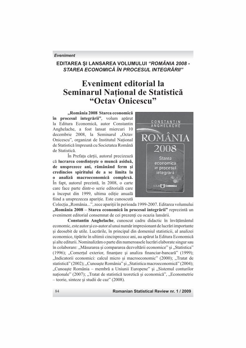
Romanian Statistical Review nr. 1 / 200984
EDITAREA ŞI LANSAREA VOLUMULUI “ROMÂNIA 2008 - STAREA ECONOMICĂ ÎN PROCESUL INTEGRĂRII”
Eveniment editorial la Seminarul Naţional de Statistică
“Octav Onicescu” „România 2008 Starea economică în procesul integrării”, volum apărut la Editura Economică, autor Constantin Anghelache, a fost lansat miercuri 10 decembrie 2008, la Seminarul „Octav Onicescu”, organizat de Institutul Naţional de Statistică împreună cu Societatea Română de Statistică. În Prefaţa cărţii, autorul precizează că lucrarea consfi nţeşte o muncă asiduă, de unsprezece ani, rămânând ferm şi credincios spiritului de a se limita la o analiză macroeconomică complexă. În fapt, autorul prezintă, în 2008, o carte care face parte dintr-o serie editorială care a început din 1999, ultima ediţie anuală fi ind a unsprezecea apariţie. Este cunoscută Colecţia „România...”, zece apariţii în perioada 1999-2007. Editarea volumului „România 2008 – Starea economică în procesul integrării” reprezintă un eveniment editorial consemnat de cei prezenţi cu ocazia lansării. Constantin Anghelache, cunoscut cadru didactic în învăţământul economic, este autor şi co-autor al unui număr impresionant de lucrări importante şi deosebit de utile. Lucrările, în principal din domeniul statisticii, al analizei economice, tipărite în ultimii cincisprezece ani, au apărut la Editura Economică şi alte editurii. Nominalizăm o parte din numeroasele lucrări elaborate singur sau în colaborare: „Măsurarea şi compararea dezvoltării economice” şi „Statistica” (1996); „Comerţul exterior, fi nanţare şi analiza fi nanciar-bancară” (1999); „Indicatorii economici: calcul micro şi macroeconomic” (2000); „Tratat de statistică” (2002); „Cunoaşte România” şi „Statistica macroeconomică” (2004); „Cunoaşte România – membră a Uniunii Europene” şi „Sistemul conturilor naţionale” (2007); „Tratat de statistică teoretică şi economică”, „Econometrie – teorie, sinteze şi studii de caz” (2008).
Eveniment
Revista Română de Statistică nr. 1 / 2009 85
Reţine atenţia prezentarea aparţinând prof. univ. dr. Marin Dinu, text apărut pe coperta cărţii lansate recent: „«România 2008 – Starea economică în procesul integrării» este un martor lucid şi dezinteresat al distanţelor care încă mai separă managementul politic de paradigmele tranziţiei şi o radiografi e coerentă cu intenţie randamentală, a problemelor care îşi aştepată rezolvarea. Prof. univ. dr. Constantin Anghelache este autorul cel mai prolifi c din România - a publicat anual lucrări similare începând cu 1999 – care fracturează credinţa încetăţenită în analizele emoţionale şi care, într-o manieră decomplexată, umanizează cercetarea ştiinţifi că şi o pune la dispoziţia celor interesaţi pentru a opera cu un grad mai ridicat de cunoaştere în actul decizional”.
PREZENTARE DE COMUNICARE În cadrul Seminarului, prof. univ. dr. Miruna Mazurencu şi conf. univ. dr. Ileana Niculescu-Aron, de la Academia de Studii Economice Bucureşti, au prezentat rezultatele parţiale ale Grantului: „Model statistico-econometric inovativ pentru detectarea timpurie a insolvabilităţii companiilor bazate pe T.I.C. şi C.D. care operează în economia de post-tranziţie a României. Implicaţii macro-economice”. Echipa de autori din care au făcut parte şi prof. univ. dr. Dana Colibabă, lector drd. Raluca Şerban şi lector drd. Anca Bogdan, a obţinut o serie de date şi informaţii de referinţă privind productivitatea companiilor în două domenii importante de activitate: Tehnologia informaţiei şi Telecomunicaţiile.
*** Organizarea Seminarului Naţional de Statistică „Octav Onicescu” din 10 decembrie 2008 cu cele două acţiuni: prezentarea comunicării menţionate şi lansarea cărţii prof. univ. dr. Constantin Anghelache, a fost inspirată. Prof. univ. dr. Vergil Voineagu, preşedintele INS, a condus lucrările Seminarului, remarcând valoarea cărţii lansate de prof. Anghelache. Pentru autorii comunicării, prof. Voineagu a recomandat să intensifi ce şi în viitor documentarea consultând şi alte publicaţii specifi ce elaborate de INS. Au făcut comentarii, exprimând şi puncte de vedere: prof. univ. dr. Marius Băcescu, ing. Adrian Nica, ec. Ioan B. Gâlceavă, prof. Ion Răvar, ec. Laurenţiu Guţescu şi ec. Ilie Dumitrescu. În fi nal, autorul volumului „România 2008 – Starea economică în procesul integrării” a acordat autografe celor prezenţi.
A consemnatEc. Ioan B. GÂLCEAVĂ
Eveniment

Romanian Statistical Review nr. 1 / 200986
Responsabil de număr: Prof. univ. dr. Constantin ANGHELACHE Echipa logistică: Nicolae IONESCU, Iancu UCEANU,
Gheorghe VAIDA-MUNTEAN, Oana BURDUŞEL, Tiberiu PREDA
Condiţii pentru prezentarea materialelor spre publicare
Lucrările ştiinţifi ce sau tehnice, originale, se pot prezenta redacţiei spre publicare fi e sub formă de articole, fi e sub formă de scurte comunicări în limba română şi în limba engleză (traducere integrală). Precizările privind condiţiile tehnice pentru predarea materialelor se afl ă pe site-ul www.revistadestatistica.ro, secţiunea „Procesul de recenzare”.
Conditions for the articles designated for the Romanian Statistical Review
The original scientifi c or technical works can be sent to be published either under article form or short communications in Romanian and English (complete translation). The technical conditions for the articles to be presented can be found at www.revistadestatistica.ro in the “Peer review” section.
Cititorii din ţară şi străinătate se pot abona prin S.C. Rodipet S.A cu sediul în
Piaţa Presei Libere nr. 1, Corp B, Sector 1, Bucureşti, România
tel/fax 0040-21-318.70.00sau e-mail: [email protected] şi [email protected]
ISSN 1018-046X
Reproducerea articolelor fără acordul Institutului Naţional de Statistică - Editura Revista Română de Statistică este interzisă, iar utilizarea conţinutului acestei publicaţii, cu titlul explicativ sau justifi cativ, în diferite lucrări este autorizată numai cu precizarea clară a sursei.
Redacţia Editurii “Revista Română de Statistică” precizează că punctele de vedere, datele şi informaţiile cuprinse în articolele publicate aparţin autorilor şi nu angajează răspunderea Institutului Naţional de Statistică
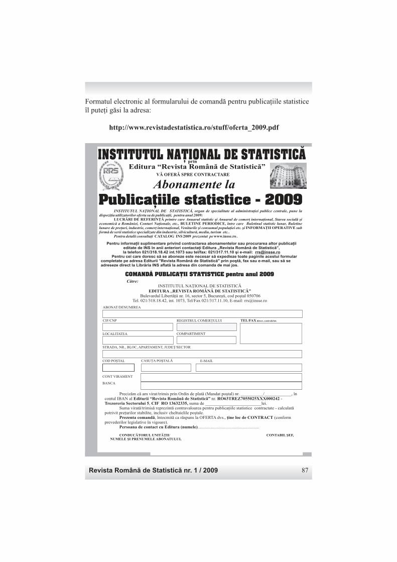
Revista Română de Statistică nr. 1 / 2009 87
Formatul electronic al formularului de comandă pentru publicaţiile statistice îl puteţi găsi la adresa: http://www.revistadestatistica.ro/stuff/oferta_2009.pdf
Editura “Revista Românã de Statisticã”
INSTITUTUL NAÞIONAL DE STATISTICÃ, organ de specialitate al administraþiei publice centrale, pune ladispoziþia utilizatorilor oferta sa de publicaþii, pentru anul 2009:
printre care Anuarul statistic ºi Anuarul de comerþ interna , Starea socialã ºieconomicã a României, Conturi Naþionale, etc., Buletinul statistic lunar, Buletinelunare de preþuri, industrie, comerþ interna ional, Veniturile ºi consumul populaþiei etc. i
din industrie, silviculturã, mediu, turism etc.Pentru detalii consultaþi prezentat pe .
LUCRÃRI DE REFERINÞÃBULETINE PERIODICE,
INFORMAÞII OPERATIVE.
CATALOG INS2009 www.insse.ro
þionalîntre
þ º subformã de serii statistice specializate
care
VÃ OFERÃ SPRE CONTRACTARE
Publicaþiile statistice - 2009
ABONAT/DENUMIREA
CIF/CNP
LOCALITATEA COMPARTIMENT
STRADA, NR., BLOC, APARTAMENT, JUDEÞ/SECTOR
COD POªTAL CASUÞA POªTALÃ
TEL/FAX direct, centralã int./
CONT VIRAMENT
BANCA
...................................................................
Precizãm cã am virat/trimis prin Ordin de platã (Mandat poºtal) nr. __________/____________, încontul IBAN al nr. -
, suma de _________________________lei.
, întocmitã ca rãspuns la OFERTA dvs., (conformprevederilor legislative în vigoare).
Editurii “Revista Românã de Statisticã” RO63TREZ7055025XXX000242Trezoreria Sectorului 5 CIF RO 13632335,
Prezenta comandã þine loc de CONTRACT
ersoana de contact cu Editura (numele)
Suma viratã/trimisã reprezintã contravaloarea pentru publicaþiile statistice contractate - calculatãpotrivit preþurilor stabilite, inclusiv cheltuielile poºtale.
P
CONDUCÃTORULUNITÃÞII/ CONTABIL ªEF,NUMELE ªI PRENUMELEABONATULUI,
Pentru informaþii suplimentare privind contractarea sau procurarea altor publicaþiieditate de INS în anii anteriori contactaþi Editura „Revista Românã de Statisticã”,la telefon 021/318.18.42 int.1073 sau tel/fax: 021/317.11.10 ºi e-mail:
Pentru cei care doresc sã se aboneze este necesar sã expedieze toate paginile acestui formularcompletate pe adresa Editurii "Revista Românã de Statisticã" prin poºtã, fax sau e-mail, sau sã seadreseze direct la Librãria INS aflatã la adresa din comanda de mai jos.
abonamentelor
INSTITUTUL NAÞIONAL DE STATISTICÃprin
Abonamente la
Cãtre:INSTITUTUL NAÞIONAL DE STATISTICÃ
Bulevardul Libertãþii nr. 16, sector 5, Bucure cod poºtal 050706Tel. 021/318.18.42, int. 1073, Tel/Fax 021/317.11.10, E-mail: [email protected]
EDITURA REVISTAROMÂNà DE STATISTICÔºti,
„
COMANDÃ PUBLICA II STATISTICE pentru anul 2009Þ
REGISTRUL COMER ULUIÞ
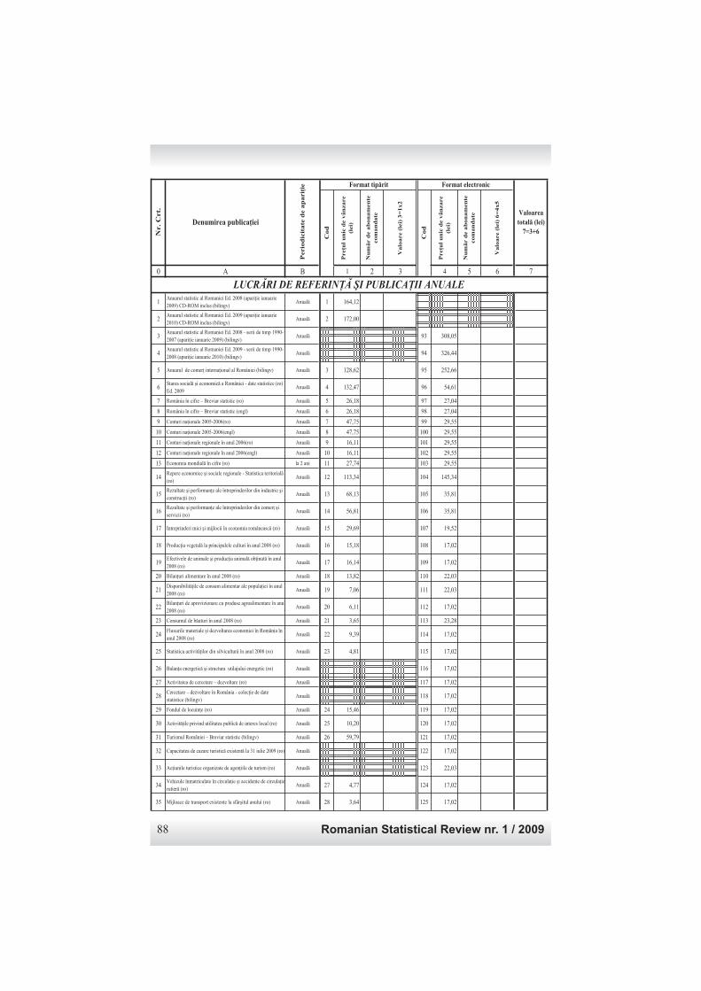
Romanian Statistical Review nr. 1 / 200988
Pre u
l u
nic
de v
ân
za
re
(lei)
Nu
m!
r d
e a
bo
na
men
te
co
ma
nd
ate
Va
loa
re (
lei)
3=
1x
2
Pre u
l u
nic
de v
ân
za
re
(lei)
Nu
m!
r d
e a
bo
na
men
te
co
ma
nd
ate
Va
loa
re (
lei)
6=
4x
5
0 A B 1 2 3 4 5 6 7
1Anuarul statistic al Romaniei Ed. 2008 (apari ie ianuarie
2009) CD-ROM inclus (bilingv)Anual! 1 164,12
2Anuarul statistic al Romaniei Ed. 2009 (apari ie ianuarie
2010) CD-ROM inclus (bilingv)Anual! 2 172,00
3Anuarul statistic al Romaniei Ed. 2008 - serii de timp 1990-
2007 (apari ie ianuarie 2009) (bilingv)Anual! 93 308,05
4Anuarul statistic al Romaniei Ed. 2009 - serii de timp 1990-
2008 (apari ie ianuarie 2010) (bilingv)Anual! 94 326,44
5 Anuarul de comer interna ional al României (bilingv) Anual! 3 128,62 95 252,66
6Starea social! "i economic! a României - date statistice (ro)
Ed. 2009Anual! 4 132,47 96 54,61
7 România în cifre – Breviar statistic (ro) Anual! 5 26,18 97 27,04
8 România în cifre – Breviar statistic (engl) Anual! 6 26,18 98 27,04
9 Conturi na ionale 2005-2006(ro) Anual! 7 47,75 99 29,55
10 Conturi na ionale 2005-2006(engl) Anual! 8 47,75 100 29,55
11 Conturi na ionale regionale în anul 2006(ro) Anual! 9 16,11 101 29,55
12 Conturi na ionale regionale în anul 2006(engl) Anual! 10 16,11 102 29,55
13 Economia mondial! în cifre (ro) la 2 ani 11 27,74 103 29,55
14Repere economice "i sociale regionale - Statistica teritorial!
(ro)Anual! 12 113,34 104 145,34
15Rezultate "i performan e ale întreprinderilor din industrie "i
construc ii (ro) Anual! 13 68,13 105 35,81
16Rezultate "i performan e ale întreprinderilor din comer "i
servicii (ro)Anual! 14 56,81 106 35,81
17 Intreprinderi mici "i mijlocii în economia româneasc! (ro) Anual! 15 29,69 107 19,52
18 Produc ia vegetal! la principalele culturi în anul 2008 (ro) Anual! 16 15,18 108 17,02
19Efectivele de animale "i produc ia animal! ob inut! în anul
2008 (ro)Anual! 17 16,14 109 17,02
20 Bilan uri alimentare în anul 2008 (ro) Anual! 18 13,82 110 22,03
21Disponibilit! ile de consum alimentar ale popula iei în anul
2008 (ro)Anual! 19 7,06 111 22,03
22Bilan uri de aprovizionare cu produse agroalimentare în anul
2008 (ro)Anual! 20 6,11 112 17,02
23 Consumul de b!uturi în anul 2008 (ro) Anual! 21 3,65 113 23,28
24Fluxurile materiale "i dezvoltarea economiei în România în
anul 2008 (ro)Anual! 22 9,39 114 17,02
25 Statistica activit! ilor din silvicultur! în anul 2008 (ro) Anual! 23 4,81 115 17,02
26 Balan a energetic! "i structura utilajului energetic (ro) Anual! 116 17,02
27 Activitatea de cercetare – dezvoltare (ro) Anual! 117 17,02
28Cercetare – dezvoltare în România - colec ie de date
statistice (bilingv)Anual! 118 17,02
29 Fondul de locuin e (ro) Anual! 24 15,46 119 17,02
30 Activit! ile privind utilitatea public! de interes local (ro) Anual! 25 10,20 120 17,02
31 Turismul României – Breviar statistic (bilingv) Anual! 26 59,79 121 17,02
32 Capacitatea de cazare turistic! existent! la 31 iulie 2009 (ro) Anual! 122 17,02
33 Ac iunile turistice organizate de agen iile de turism (ro) Anual! 123 22,03
34Vehicule înmatriculate în circula ie "i accidente de circula ie
rutier! (ro)Anual! 27 4,77 124 17,02
35 Mijloace de transport existente la sfâr"itul anului (ro) Anual! 28 3,64 125 17,02
Denumirea publica iei
Nr.
Crt.
Perio
dic
ita
te d
e a
pa
ri
ie
Co
d
Valoarea
total! (lei)
7=3+6
Format tip!rit
Co
d
Format electronic
LUCR RI DE REFERIN! "I PUBLICA!II ANUALE
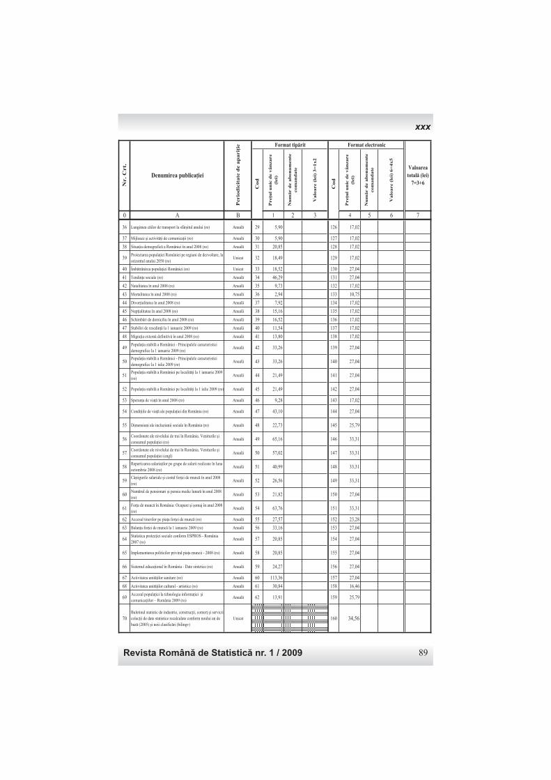
Revista Română de Statistică nr. 1 / 2009 89
xxx
Pre u
l u
nic
de v
ân
za
re
(lei)
Nu
m!
r d
e a
bo
na
men
te
co
ma
nd
ate
Va
loa
re (
lei)
3=
1x
2
Pre u
l u
nic
de v
ân
za
re
(lei)
Nu
m!
r d
e a
bo
na
men
te
co
ma
nd
ate
Va
loa
re (
lei)
6=
4x
5
0 A B 1 2 3 4 5 6 7
Denumirea publica iei
Nr.
Crt.
Perio
dic
ita
te d
e a
pa
ri
ie
Co
d
Valoarea
total! (lei)
7=3+6
Format tip!rit
Co
d
Format electronic
36 Lungimea c ilor de transport la sfâr!itul anului (ro) Anual 29 5,90 126 17,02
37 Mijloace !i activit "i de comunica"ii (ro) Anual 30 5,90 127 17,02
38 Situa"ia demografic a României în anul 2008 (ro) Anual 31 20,85 128 17,02
39Proiectarea popula"iei României pe regiuni de dezvoltare, la orizontul anului 2050 (ro)
Unicat 32 18,49 129 17,02
40 Îmb trânirea popula"iei României (ro) Unicat 33 18,52 130 27,04
41 Tendin"e sociale (ro) Anual 34 46,29 131 27,04
42 Natalitatea în anul 2008 (ro) Anual 35 9,73 132 17,02
43 Mortalitatea în anul 2008 (ro) Anual 36 2,94 133 10,75
44 Divor"ialitatea în anul 2008 (ro) Anual 37 7,92 134 17,02
45 Nup"ialitatea în anul 2008 (ro) Anual 38 15,16 135 17,02
46 Schimb ri de domiciliu în anul 2008 (ro) Anual 39 16,52 136 17,02
47 Stabiliri de resedin" la 1 ianuarie 2009 (ro) Anual 40 11,54 137 17,02
48 Migra"ia extern definitiv în anul 2008 (ro) Anual 41 13,80 138 17,02
49Popula"ia stabil a României - Principalele caracteristici demografice la 1 ianuarie 2009 (ro)
Anual 42 33,26 139 27,04
50Popula"ia stabil a României - Principalele caracteristici demografice la 1 iulie 2009 (ro)
Anual 43 33,26 140 27,04
51Popula"ia stabil a României pe localit "i la 1 ianuarie 2009 (ro)
Anual 44 21,49 141 27,04
52 Popula"ia stabil a României pe localit "i la 1 iulie 2009 (ro) Anual 45 21,49 142 27,04
53 Speran"a de via" în anul 2008 (ro) Anual 46 9,28 143 17,02
54 Condi"iile de via" ale popula"iei din România (ro) Anual 47 43,10 144 27,04
55 Dimensiuni ale incluziunii sociale în România (ro) Anual 48 22,73 145 25,79
56Coordonate ale nivelului de trai în România. Veniturile !iconsumul popula"iei (ro)
Anual 49 65,16 146 33,31
57Coordonate ale nivelului de trai în România. Veniturile !iconsumul popula"iei (engl)
Anual 50 57,02 147 33,31
58Repartizarea salaria"ilor pe grupe de salarii realizate în luna octombrie 2008 (ro)
Anual 51 40,99 148 33,31
59Câ!tigurile salariale !i costul for"ei de munc în anul 2008 (ro)
Anual 52 26,56 149 33,31
60Num rul de pensionari !i pensia medie lunar în anul 2008 (ro)
Anual 53 21,82 150 27,04
61For"a de munc în România: Ocupare !i !omaj în anul 2008 (ro)
Anual 54 63,76 151 33,31
62 Accesul tinerilor pe pia"a for"ei de munc (ro) Anual 55 27,57 152 23,28
63 Balan"a for"ei de munc la 1 ianuarie 2009 (ro) Anual 56 33,16 153 27,04
64Statistica protec"iei sociale conform ESPROS - România 2007 (ro)
Anual 57 20,85 154 27,04
65 Implementarea politicilor privind pia"a muncii - 2008 (ro) Anual 58 20,85 155 27,04
66 Sistemul educa"ional în România - Date sintetice (ro) Anual 59 24,27 156 27,04
67 Activitatea unit "ilor sanitare (ro) Anual 60 113,36 157 27,04
68 Activitatea unit "ilor cultural - artistice (ro) Anual 61 30,84 158 16,46
69Accesul popula"iei la tehnologia informa"iei !icomunica"iilor – România 2009 (ro)
Anual 62 13,91 159 25,79
70Buletinul statistic de industrie, construc"ii, comer" !i servicii colec"ii de date statistice recalculate conform noului an de baz (2005) !i noii clasific ri (bilingv)
Unicat 160 34,56
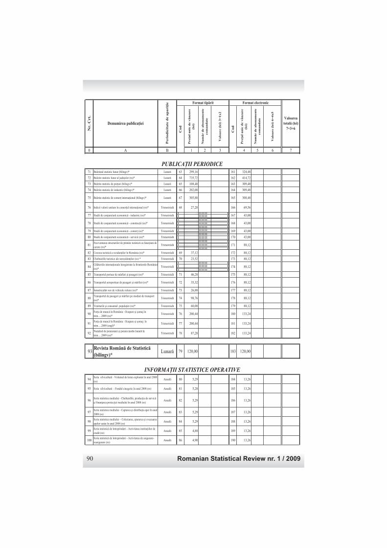
Romanian Statistical Review nr. 1 / 200990
Pre u
l u
nic
de v
ân
za
re
(lei)
Nu
m!
r d
e a
bo
na
men
te
co
ma
nd
ate
Va
loa
re (
lei)
3=
1x
2
Pre u
l u
nic
de v
ân
za
re
(lei)
Nu
m!
r d
e a
bo
na
men
te
co
ma
nd
ate
Va
loa
re (
lei)
6=
4x
5
0 A B 1 2 3 4 5 6 7
Denumirea publica iei
Nr.
Crt.
Perio
dic
ita
te d
e a
pa
ri
ie
Co
d
Valoarea
total! (lei)
7=3+6
Format tip!rit
Co
d
Format electronic
71 Buletinul statistic lunar (bilingv)* Lunar 63 299,16 161 324,48
72 Buletin statistic lunar al jude!elor (ro)* Lunar 64 735,72 162 414,72
73 Buletin statistic de pre!uri (bilingv)* Lunar 65 108,48 163 309,48
74 Buletin statistic de industrie (bilingv)* Lunar 66 202,08 164 309,48
75 Buletin statistic de comer! interna!ional (bilingv)* Lunar 67 305,88 165 308,48
76 Indicii valorii unitare în comer!ul interna!ional (ro)* Trimestrial 68 27,28 166 69,56
77 Studii de conjunctur economic - industrie (ro)* Trimestrial 167 43,00
78 Studii de conjunctur economic - construc!ii (ro)* Trimestrial 168 43,00
79 Studii de conjunctur economic - comer! (ro)* Trimestrial 169 43,00
80 Studii de conjunctur economic - servicii (ro)* Trimestrial 170 43,00
81Frecventarea structurilor de primire turistic cu func!iuni de cazare (ro)*
Trimestrial 171 88,12
82 Cererea turistic a reziden!ilor în România (ro)* Trimestrial 69 37,12 172 88,12
83 Cheltuielile turistice ale nereziden!ilor (ro) * Trimestrial 70 23,52 173 88,12
84C l toriile interna!ionale înregistrate la frontierele României (ro)*
Trimestrial 174 88,12
85 Transportul portuar de m rfuri "i pasageri (ro)* Trimestrial 71 46,28 175 88,12
86 Transportul aeroportuar de pasageri "i m rfuri (ro)* Trimestrial 72 35,32 176 88,12
87 Înmatricul ri noi de vehicule rutiere (ro)* Trimestrial 73 26,88 177 88,12
88Transportul de pasageri "i m rfuri pe moduri de transport (ro)*
Trimestrial 74 98,76 178 88,12
89 Veniturile "i consumul popula!iei (ro)* Trimestrial 75 60,08 179 88,12
90For!a de munc în România : Ocupare "i "omaj în trim.....2009 (ro)*
Trimestrial 76 200,44 180 133,24
91For!a de munc în România : Ocupare "i "omaj în trim.....2009 (engl)*
Trimestrial 77 200,44 181 133,24
92Num rul de pensionari "i pensia medie lunar în trim.....2009 (ro)*
Trimestrial 78 87,28 182 133,24
93Revista Român! de Statistic!
(bilingv)*Lunar 79 120,00 183 120,00
94Seria silvicultur -Volumul de lemn exploatat în anul 2008 (ro)
Anual 80 5,29 184 13,26
95 Seria silvicultur - Fondul cinegetic în anul 2008 (ro) Anual 81 5,28 185 13,26
96Seria statistica mediului - Cheltuielile, produc!ia de servicii "i finan!area protec!iei mediului în anul 2008 (ro)
Anual 82 5,29 186 13,26
97Seria statistica mediului - Captarea "i distribu!ia apei în anul 2008 (ro)
Anual 83 5,29 187 13,26
98Seria statistica mediului – Colectarea, epurarea "i evacuarea apelor uzate în anul 2008 (ro)
Anual 84 5,29 188 13,26
99Seria statistic de întreprinderi - Activitatea institu!iilor de credit (ro)
Anual 85 4,88 189 13,26
100Seria statistic de întreprinderi - Activitatea de asigurare-reasigurare (ro)
Anual 86 4,90 190 13,26
INFORMA!II STATISTICE OPERATIVE
PUBLICA!II PERIODICE
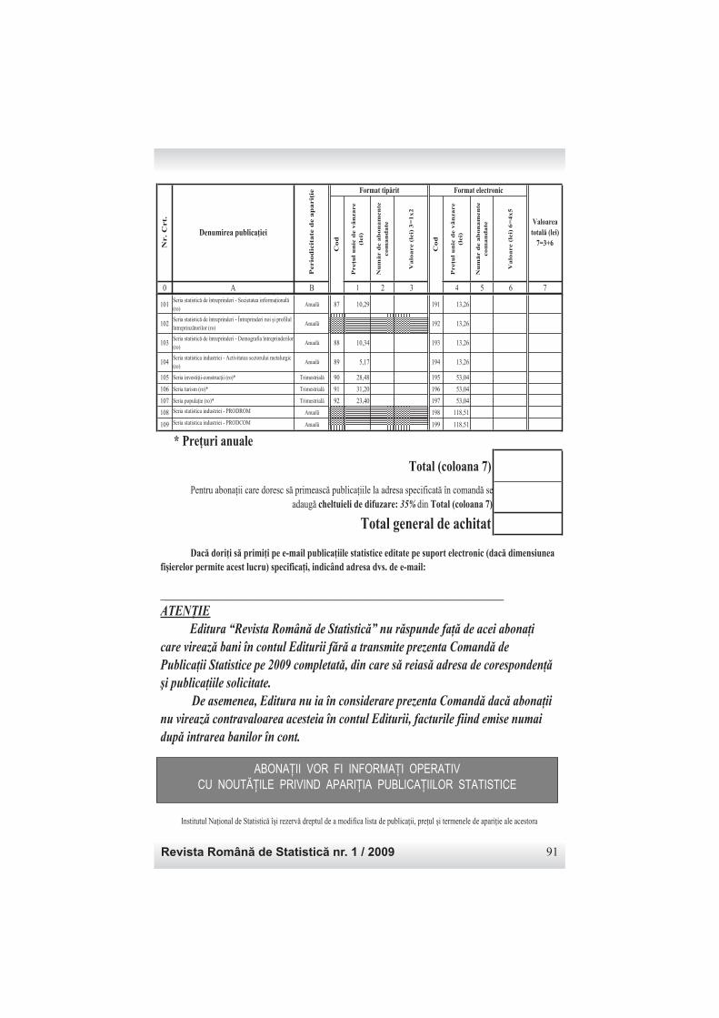
Revista Română de Statistică nr. 1 / 2009 91
Pre u
l u
nic
de v
ân
za
re
(lei)
Nu
m!
r d
e a
bo
na
men
te
co
ma
nd
ate
Va
loa
re (
lei)
3=
1x
2
Pre u
l u
nic
de v
ân
za
re
(lei)
Nu
m!
r d
e a
bo
na
men
te
co
ma
nd
ate
Va
loa
re (
lei)
6=
4x
5
0 A B 1 2 3 4 5 6 7
Denumirea publica iei
Nr.
Crt.
Perio
dic
ita
te d
e a
pa
ri
ie
Co
d
Valoarea
total! (lei)
7=3+6
Format tip!rit
Co
d
Format electronic
101Seria statistic de întreprinderi - Societatea informa!ional (ro)
Anual 87 10,29 191 13,26
102Seria statistic de întreprinderi - Întreprinderi noi "i profilul întreprinz torilor (ro)
Anual 192 13,26
103Seria statistic de întreprinderi - Demografia întreprinderilor (ro)
Anual 88 10,34 193 13,26
104Seria statistica industriei - Activitatea sectorului metalurgic (ro)
Anual 89 5,17 194 13,26
105 Seria investi!ii-construc!ii (ro)* Trimestrial 90 28,48 195 53,04
106 Seria turism (ro)* Trimestrial 91 31,20 196 53,04
107 Seria popula!ie (ro)* Trimestrial 92 23,40 197 53,04
108 Seria statistica industriei - PRODROM Anual 198 118,51
109 Seria statistica industriei - PRODCOM Anual 199 118,51
* Pre uri anuale
Institutul Na!ional de Statistic î"i rezerv dreptul de a modifica lista de publica!ii, pre!ul "i termenele de apari!ie ale acestora
Pentru abona!ii care doresc s primeasc publica!iile la adresa specificat în comand seadaug cheltuieli de difuzare: 35% din Total (coloana 7)
Total general de achitat
Total (coloana 7)
Dac! dori i s! primi i pe e-mail publica iile statistice editate pe suport electronic (dac! dimensiunea
fi"ierelor permite acest lucru) specifica i, indicând adresa dvs. de e-mail:
________________________________________________________________________________
ATEN!IE
Editura “Revista Român" de Statistic"” nu r"spunde fa#" de acei abona#icare vireaz" bani în contul Editurii f"r" a transmite prezenta Comand" de
Publica#ii Statistice pe 2009 completat", din care s" reias" adresa de coresponden#"$i publica#iile solicitate.
De asemenea, Editura nu ia în considerare prezenta Comand" dac" abona#iinu vireaz" contravaloarea acesteia în contul Editurii, facturile fiind emise numai
dup" intrarea banilor în cont.
ABONA II VOR FI INFORMA I OPERATIV
CU NOUT! ILE PRIVIND APARI IA PUBLICA IILOR STATISTICE