Optimizare s i analiza statistica˘ a datelor privind...
42
Universitatea din Bucures , ti F acultatea de Matematic ˘ as , i Informatic ˘ a Tez ˘ a de doctorat Rezumat Optimizare s , i analiza statistic ˘ a a datelor privind durata de viat , ˘ a Doctorand: Mircea Dr ˘ agulin Conduc˘ ator S , tiint , ific: Prof. Dr. Vasile Preda Bucures , ti 2014
Transcript of Optimizare s i analiza statistica˘ a datelor privind...
Universitatea din Bucures,ti
Facultatea deMatematica s, i Informatica
Teza de doctorat
Rezumat
Optimizare s, i analiza statistica a datelorprivind durata de viat, a
Doctorand:Mircea Dragulin
Conducator S, tiint, ific:Prof. Dr. Vasile Preda
Bucures, ti 2014
Cuprins
Cuprins 1
1 Introducere 31.1 Actualitatea temei . . . . . . . . . . . . . . . . . . . . . . . . . . . . . . . . . . . . . 31.2 Obiectivele lucrarii . . . . . . . . . . . . . . . . . . . . . . . . . . . . . . . . . . . . 41.3 Noutatea s, tiint, ifica . . . . . . . . . . . . . . . . . . . . . . . . . . . . . . . . . . . . 41.4 Structura tezei de doctorat . . . . . . . . . . . . . . . . . . . . . . . . . . . . . . . . 5
2 Repartit, ia Lindley 8
3 Repartit, ia Lindley generalizata 93.1 Proprietat, i . . . . . . . . . . . . . . . . . . . . . . . . . . . . . . . . . . . . . . . . . 9
3.1.1 Rata de hazard s, i media de viat, a reziduala . . . . . . . . . . . . . . . . . . 93.1.2 Momentele, media s, i dispersia . . . . . . . . . . . . . . . . . . . . . . . . . 93.1.3 Transformata Laplace-Stieltjes s, i convolut, ii . . . . . . . . . . . . . . . . . . 103.1.4 Entropia Shannon. Caracterizare . . . . . . . . . . . . . . . . . . . . . . . . 103.1.5 Entropia Renyi . . . . . . . . . . . . . . . . . . . . . . . . . . . . . . . . . . 10
3.2 Estimare s, i generare de date . . . . . . . . . . . . . . . . . . . . . . . . . . . . . . . 103.3 Statistici de ordine . . . . . . . . . . . . . . . . . . . . . . . . . . . . . . . . . . . . 11
3.3.1 Momentele statisticilor de ordine . . . . . . . . . . . . . . . . . . . . . . . . 113.3.2 Momentele statisticilor de ordine trunchiate . . . . . . . . . . . . . . . . . 11
3.4 Estimarea bayesiana s, i non-bayesiana pentru doua populat, ii Lindley generalizatfolosind schema comuna de cenzurare de tipul II . . . . . . . . . . . . . . . . . . . 123.4.1 Estimatori de verosimilitate maxima . . . . . . . . . . . . . . . . . . . . . . 123.4.2 Intervale de ıncredere bootstrap . . . . . . . . . . . . . . . . . . . . . . . . 133.4.3 Estimatori bayesieni . . . . . . . . . . . . . . . . . . . . . . . . . . . . . . . 133.4.4 Estimarea fiabilitat, ii stres-rezistent, a R = P(Y < X) . . . . . . . . . . . . . . 13
4 Repartit, ia putere a unei variabile aleatoare repartizata Lindley generalizat 144.1 Proprietat, i . . . . . . . . . . . . . . . . . . . . . . . . . . . . . . . . . . . . . . . . . 14
4.1.1 Rata de hazard . . . . . . . . . . . . . . . . . . . . . . . . . . . . . . . . . . 144.1.2 Momentele, media s, i dispersia . . . . . . . . . . . . . . . . . . . . . . . . . 144.1.3 Entropia Renyi . . . . . . . . . . . . . . . . . . . . . . . . . . . . . . . . . . 14
4.2 Generarea de date . . . . . . . . . . . . . . . . . . . . . . . . . . . . . . . . . . . . . 154.3 Statistici de ordine . . . . . . . . . . . . . . . . . . . . . . . . . . . . . . . . . . . . 154.4 Estimatori de verosimilitate maxima . . . . . . . . . . . . . . . . . . . . . . . . . . 15
1
5 Repartit, ii mixate ale duratelor de viat, a 165.1 Repartit, ia Lindley generalizat Poisson Max . . . . . . . . . . . . . . . . . . . . . . 16
5.1.1 Proprietat, i . . . . . . . . . . . . . . . . . . . . . . . . . . . . . . . . . . . . . 165.1.2 Entropia Shannon. Caracterizare . . . . . . . . . . . . . . . . . . . . . . . . 175.1.3 Generarea de date . . . . . . . . . . . . . . . . . . . . . . . . . . . . . . . . 18
5.2 Repartit, ia Lindley generalizat Poisson Min . . . . . . . . . . . . . . . . . . . . . . 185.2.1 Proprietat, i . . . . . . . . . . . . . . . . . . . . . . . . . . . . . . . . . . . . . 185.2.2 Entropia Shannon. Caracterizare . . . . . . . . . . . . . . . . . . . . . . . . 195.2.3 Generarea de date . . . . . . . . . . . . . . . . . . . . . . . . . . . . . . . . 19
5.3 Repartit, ia Lindley generalizat Binomial Max . . . . . . . . . . . . . . . . . . . . . 195.3.1 Proprietat, i . . . . . . . . . . . . . . . . . . . . . . . . . . . . . . . . . . . . . 205.3.2 Entropia Shannon. Caracterizare . . . . . . . . . . . . . . . . . . . . . . . . 205.3.3 Generarea de date . . . . . . . . . . . . . . . . . . . . . . . . . . . . . . . . 21
5.4 Repartit, ia Lindley generalizat Binomial Min . . . . . . . . . . . . . . . . . . . . . 215.4.1 Proprietat, i . . . . . . . . . . . . . . . . . . . . . . . . . . . . . . . . . . . . . 215.4.2 Entropia Shannon. Caracterizare . . . . . . . . . . . . . . . . . . . . . . . . 225.4.3 Generarea de date . . . . . . . . . . . . . . . . . . . . . . . . . . . . . . . . 23
5.5 Repartit, ia Lindley generalizat Geometric Max . . . . . . . . . . . . . . . . . . . . 235.5.1 Proprietat, ii . . . . . . . . . . . . . . . . . . . . . . . . . . . . . . . . . . . . 235.5.2 Entropia Shannon. Caracterizare . . . . . . . . . . . . . . . . . . . . . . . . 245.5.3 Generarea de date . . . . . . . . . . . . . . . . . . . . . . . . . . . . . . . . 24
5.6 Repartit, ia Lindley generalizat Geometric Min . . . . . . . . . . . . . . . . . . . . . 245.6.1 Proprietat, i . . . . . . . . . . . . . . . . . . . . . . . . . . . . . . . . . . . . . 255.6.2 Entropia Shannon. Caracterizare . . . . . . . . . . . . . . . . . . . . . . . . 255.6.3 Generarea de date . . . . . . . . . . . . . . . . . . . . . . . . . . . . . . . . 26
6 Procese de reınnoire 276.1 Procese de reınnoire . . . . . . . . . . . . . . . . . . . . . . . . . . . . . . . . . . . . 276.2 Procese de reınnoire s, i repartit, ia Lindley generalizat Poisson Min . . . . . . . . . 27
6.2.1 Durata reınnoirilor la momentul t . . . . . . . . . . . . . . . . . . . . . . . 276.3 Procese de reınnoire s, i repartit, ia Lindley generalizat Binomial Min . . . . . . . . 28
6.3.1 Durata reınnoirilor la momentul t . . . . . . . . . . . . . . . . . . . . . . . 28
7 Optimizarea unor sisteme 297.1 Fiabilitatea sistemelor serie, paralel s, i k-out-of-n pentru durate de viat, a variabile
aleatoare independente identic repartizate Lindley generalizat . . . . . . . . . . . 297.2 Model Cox D.R., Nakagawa T. de acumulare pentru daune independente identic
repartizate Lindley generalizat . . . . . . . . . . . . . . . . . . . . . . . . . . . . . 307.2.1 Optimizarea costurilor cu daune independente identic repartizate Lind-
ley generalizat . . . . . . . . . . . . . . . . . . . . . . . . . . . . . . . . . . . 317.3 Model de mentenant, a Lam Y., Zhang Y.L. cu timpi de funct, ionare (Xn)n independent, i
identic repartizat, i Lindley generalizat . . . . . . . . . . . . . . . . . . . . . . . . . 317.4 Ret, elele Ad-Hoc ZRP Ben Liang, Zgymunt J. Haas pentru durate Lindley gene-
ralizat ale legaturilor up s, i down . . . . . . . . . . . . . . . . . . . . . . . . . . . . 32
Bibliografie 34
2
Capitolul 1
Introducere
Analiza duratelor de viat, a este o ramura extinsa s, i populara fiind folosita ın multe domeniicum ar fi medicina, inginerie, asigurari, industrie, economie, management, s, tiint, ele mediului s, is, tiint, ele sociale. De exemplu, ın studiul potent, ialului risc de moarte cauzat de boala, de intereseste timpul de supraviet, uire a bolnavilor, masurat de la data diagnosticului, sau comparareatratamentelor pentru o boala ın termeni de repartit, ii de supraviet, uire pentru pacient, ii careprimesc tratamente diferite. Un alt exemplu este interesul demografilor pentru durata uneianumite ”stari” cum ar fi casatoria. Se alege un an s, i se contabilizeaza casatoriile din acel an.De interes este durata casatoriei care poate sa se ıncheie cu anulare, divort, sau moartea unuiadin parteneri. Un exemplu important este din industrie. Rezistent, a materialelor sau a unorcomponete dintr-un sistem este observata ın condit, ii de laborator pana cand acestea cedeaza.Duratele de viat, a ın acest caz se mai numesc s, i durate de defect, iune deoarece cand un obiectınceteaza sa mai funct, ioneze corespunzator, spunem ca s-a defectat Jerald F. Lawless [79].
Multe modele statistice cat s, i metode de analiza a datelor de supraviet, uire au fost dezvol-tate de-a lungul timpului. Astfel pentru ultimul exemplu, o repartit, ie care modeleaza cedareamaterialelor este repartit, ia Birnbaum Saunders [22, 23]. Dar cea mai utilizata s, i raspanditarepartit, ie asociata datelor de supraviet, uire este cea exponent, iala. Alte repartit, ii folosite suntrepartit, ia gamma, Weibull s, i log-normal Barlow R.E., Proschan F. [16].
1.1 Actualitatea temei
Datorita dezvoltarii rapide a tehnologiei s, i a sistemelor, a aparut necesitatea dezvol-tarii denoi modele matematice asupra duratelor de viat, a s, i aplicarea acestora ın cadrul proceselorstocastice, ın particular asupra proceselor de reınnoire. Procesele de reınnoire sunt importanteın fiabilitate s, i mentenant, a sistemelor, un obiectiv de urmarit fiind: cand ar trebui schim-bate piesele s, i cate piese de schimb ar trebui sa avem ın depozit la fiecare moment t?. Inmulte situat, ii, defect, iunea unei piese ın timpul activitat, ii este costisitoare s, i periculoasa. Dacapiesa respectiva este caracterizata de rate de defect, iune (rate de hazard) care cresc cu timpul,este ıntelept sa ınlocuim unitatea ınainte de a se uza prea mult Barlow R.E., Proschan F. [16].Repartit, ia exponent, iala des, i cea mai raspandita s, i populara ın analiza duratelor de viat, a nueste cea mai potrivita ın teoria proceselor de reınnoire deoarece rata de hazard care ne daprobabilitatea de defect, iune imediata a unui obiect de varsta x, notata de obicei cu h(x), esteconstanta. Inseamna ca probabilitatea de defect, iune imediata a unui obiect care are repartit, iaviet, ii, repartit, ia exponent, iala, nu depinde de varsta acestuia, ceea ce face ca problemele mate-
3
matice aparute sa fie triviale Cox D.R. [30]. In cazul acesta, procesul de reınnoire, este procesulPoisson. Alte repartit, ii folosite sunt repartit, ia Weibull, repartit, ia Birnbaum Saunders (problemede vibrat, ii), repartit, ia gamma propusa de Z. W. Birnbaum s, i Saunders pentru modelarea pro-blemelor de rezistent, a ın anumite cazuri Barlow R.E., Proschan F. [16].
Recent, Ghitany M.E., Atieh B., S. Nadarajah [63] au aratat ca repartit, ia Lindley introdusa ın1958 [85, 86] este un model matematic mai bun decat repartit, ia exponent, iala pentru modela-rea datelor de viat, a, repartit, ia Lindley fiind cu proprietat, i matematice mai flexibile decat ceaexponent, iala s, i are rata de hazard crescatoarea-cu cat este mai ın varsta componenta cu atat estemai probabil ca defect, iunea sa aiba loc imediat. Dar, ın cadrul sistemelor de viat, a este mai plau-zibil ca rata de hazard sa aiba forme diferite ın funct, ie de parametrii, nu doar sa fie crescatoare,descrescatoare s, i sa fie sau unimodala sau bimodala Gayan Warahena-Liyatange, Mavis Pararai[61]. Astfel a aparut necesitatea determinarii de noi repartit, ii de viat, a care sa fie mai flexibile,cu rate de hazard de forme diferite s, i care sa modeleze cat mai multe situat, ii. Considerandacestea obiectivul lucrarii este de a introduce s, i cerceta noi modele matematice ale duratelorde viat, a pornind de la repartit, ia Lindley, prin intermediul metodelor statistico-matematice s, iaplicarea acestora ın cadrul teoriei proceselor de reınnnoire s, i la unele probleme de optimizare.
1.2 Obiectivele lucrarii
1. Construirea unei familii mai generale de repartitt, ii de tip Lindley pe baza careia se obt, inrezultatele originale ale tezei
2. Deducerea repartit, iei unor variabile aleatoare ce reprezinta maximul sau minimul a unuinumar aleator de variabile aleatoare independente identic repartizate
3. Stabilirea proprietat, ilor matematice ale acestor repartit, ii
4. Obt, inerea unor algoritmi de generare pentru aceste repartit, ii
5. Aplicarea rezultatelor obt, inute ın cadrul teoriei proceselor de reınnoire
6. Optimizarea unor sisteme de fiabilitate, modele de mentenant, a
1.3 Noutatea s, tiint,ifica
Pornind de la repartit, ia Lindley, ın literatura au aparut noi repartit, ii cum ar fi o generalizarea repartit, iei Lindley cu proprietat, ile ratei de hazard mai bune decat celei a repartit, iei gamma,lognormal sau Weibull Nadarajah S., Hassan S., Bakouch, Rasool Tahmasbi [114], repartit, ia discretPoisson-Lindley Sankaran M. [113], repartit, ia exponent, iala Poisson Lindley introdusa ın 2013de catre Barreto-Souza s, i Bakouch [18], repartit, ia zero trunchiata Poisson Lindley Ghitany M.E.,Al-Mutairi D.K., Nadarajah S. [64], ultimele doua cu aplicat, ii ın fiabilitate s, i asigurari. Altarepartit, ie introdusa recent, ın 2012, este repartit, ia Lindley geometrica cu aplicat, ii ın fiabiliate s, isupraviet, uire Hojjatollah Zakerzadeh, Eisa Mahmoudi [76]. O alta generalizare este cea propusaın 2013, care se reduce nu numai la repartit, ia Lindley ci s, i la repartit, ia exponent, iala RamaShanker, Shambhu, Ravi Shanker [106]. Alta idee de a determina alte repartit, ii este de a aplica otransformare putere, astfel a aparut repartit, ia putere Lindley Ghitany M.E., Al-Mutairi D.K., Ba-lakrishnan N., Al-Enezi [65] s, i repartit, ia exponent, iala putere Lindley Samir K., Ashour, Mahmoud
4
A., Eltehiwy [112], ultima ca o alternativa la repartit, iile gamma, Weibull, Lindley exponent, ialas, i lognormala.Alte repartit, ii aparute sunt repartit, a Lindley negativ binomiala (2010 Hassein Zamani, NoriszuraIsmail [77], Dominique Lord, Srinivas Reddy Geedipally [38]), repartit, ia quasi Lindley geometrica(2014 Diab L.S., Hiba Z. Muhammed [37]), repartit, a Lindley de doi parametri propusa de GhitannyM.E., Alqallaf F., Al-Mutairi D.K., Husain H.A. (2011 [66]) s, i repartit, ia Lindley Beta (2014 FatonMerovcis, Vikas Kumar Sharma [54]).
Noutatea s, tiint, ifica din aceasta lucrarea este introducerea de noi repartit, ii pornind de larepartit, ia Lindley, repartit, i cu proprietat, i matematice mai flexibile s, i cu rate de hazard de formediferite ın funct, ie de valorile parametrilor facand posibila modelarea multor date de viat, a. Aufost de asemenea propus, i algoritmi de simulare statistica, dar s, i metode de estimare a parame-trilor. Aceleas, i modele au fost abordate, cercetate s, i prin metode specifice teoriei proceselor dereınnoire.
Astfel, am introdus o noua generalizare a repartit, iei Lindley cat s, i transformata sa putere.Deoarece posibilitatea de a determina repartit, ia duratei de viat, a a unui sistem este aceea dea o exprima ca maximul sau minimul unui vector aleator ale carei componente caracterizeazaduratele de viat, a ale subunitat, ilor sistemului respectiv, am mixat noua repartit, ie Lindley ge-neralizata cu repart, iile zero trunchiate Poisson, binomial s, i geometric. Rezultatele obt, inute aufost aplicate ın cadrul proceselor de reınnoire.
Aplicat, ii
Rezultatele lucrarii pot fi aplicate la analiza s, i proiectarea unor sisteme ın fiabilitate s, imentenant, a sistemelor cu durata viet, ii caracterizata de noile repartit, ii determinate: repartit, iaLindley generalizata, repartit, ia Lindley generalizata putere, repartit, ia Lindley generalizata Poisson Max,repartit, ia Lindley generalizata Poisson Min, repartit, ia Lindley generalizata Binomial Max, repartit, iaLindley generalizata Binomial Min, repartit, ia Lindley generalizata Geometric Max s, i repartit, ia Lind-ley generalizata Geometric Min. Modelele matematice propuse pot servi ın calitate de modeleutilizate la descrierea unor date statistice, privin duratele de supraviet, uire de viat, a.
1.4 Structura tezei de doctorat
Lucrarea cont, ine 7 capitole s, i Bibliografie, primul capitol fiind introducerea.
In capitolul al doilea este prezentata repartit, ia Lindley ımpreuna cu cateva proprietat, i.Acest capitol se bazeaza pe lucrarile: Lindley [85, 86], Ghitany M.D., B. Atieh s, i Nadarajah S.[63].
In capitolul al treilea generalizam repartit, ia Lindley. Pentru aceasta repartit, ie sunt stabi-lite proprietat, i matematice pornind de la lucrarile [29, 63]
1. determinarea ratei de hazard s, i a mediei de viat, a reziduala
2. stabilirea momentelor de ordine r, media s, i dispersia, momentelor centrate de ordine r
3. determinarea transformatei Laplace-Stieltjes s, i a convolut, iilor
4. entropia Shannon, caracterizare
5
5. entropia Renyi
6. determinarea unor algoritmi de generare de date pentru noua repartit, ie Lindley gene-ralizata
7. estimarea parametrilor
Deoarece statisticile de ordine sunt importante ın cadrul studiului repartit, iilor, pornind dela rezultatele obt, inute de catre Gokhan Gokdere (2014 [69]), Nadarajah (2010 [92]), Bekci (2009[21]), Afity (2006 [2]), Childs s, i Balakrishnan (1998 [27]), Arnold B.C., Balakrishnan N., NagarajaH.N.(1992 [6]), Joshi s, i Balakrishnan N. (1982 [11]) au fost determinate statisticile de ordine,momentele statisticilor de ordine, statisticile de ordine trunchiate s, i momentele statisticilorde ordine trunchiate pentru repartit, ia Lindley generalizat.
Alt rezultat original pornind de la repartit, ia Lindley generalizata este estimarea bayesianas, i non-bayesiana pentru doua populat, ii Lindley generalizat folosind schema comuna decenzurare de tipul II, determinandu-se pentru parametrii s, i fiabilitate intervale de ıncredere.Astfel se extind mai multe lucrari recente. Acest capitol are la baza lucrarile Dragulin M. [39].,Dragulin M., Preda V. [40], Dragulin M., Trandafir R. [41], Dragulin M. [43], Dragulin M., Tran-dafir R., Preda V. [45], Dragulin M., Bancescu I. [46].
Capitolul al patrulea prezinta repartit, ia putere a unei variabile aleatoare repartizata Lindleygeneralizat abordare folosita recent pentru alta densitate de repartit, ie de Ghitany M.E., Al-Muhairi D.K., Balakrishnan N., Al-Enzei (2013 [65]). Acest capitol are la baza lucrarile DragulinM. [43], Dragulin M., Trandafir R. [41], Dragulin M., Preda V. [40]. S-au stabilit noi rezultateprivind
1. rata de hazard
2. momentele, media s, i dispersia
3. entropia Renyi
4. algoritm de generare de date
5. statistici de ordine-repartit, iile asimptotice
6. estimatori de verosimilitate maxima
Capitolul al cincelea are la baza lucrarile Dragulin M., Preda V. [39], Dragulin M., TrandafirR. [41], Dragulin M. [43], Dragulin M. [47]. In acest capitol au fost mixata repartit, ia Lindleygeneralizata cu repartit, iile Poisson zero trunchiata, Binomial zero trunchiata s, i Geometriczero trunchiata obt, inandu-se noi repartit, ii
1. Repartit, ia Lindley generalizat Poisson Min s, i Max
2. Repartit, ia Lindley generalizat Binomial Min s, i Max
3. Repartit, ia Lindley generalizat Geometric Min s, i Max
6
Pentru fiecare din aceste repartit, ii au fost determinat, i algoritmi de generare de date, ratade hazard, momentele, media s, i dispersia, transformata Laplace-Stieltjes, entropia Shannons, i teoreme de tip Shannon, entropia Renyi. De asemenea s-au obt, inut teoreme de tip Poissonpentru repartit, iile Lindley generalizat Binomial Min s, i Poisson Min.
Capitolul al s, aselea are la baza Dragulin M., Preda V. [40], Dragulin M., Trandafir R., [41],Dragulin M. [43], Dragulin M. [47] Dragulin M., Bancescu I., Dedu S. [48]. Acest capitol prezintaın sect, iunea 6.1 not, iuni generale pentru procese de reınnoire-Lam Y. (2007 [83]), Barlow R.E.,Proschan F., Hunter L.C. (1987 [16]), Ross M. (1996 [111]), Vaduva I. ([125]). In celelalte sect, iunis-au obt, inut noi procese de reınnoire de tip Lindley generalizat Poisson Min s, i procese dereınnoire de tip Binomial Min.
Capitolul al s, aptelea are la baza Dragulin M., Preda V. [40], Dragulin M., Trandafir R.,[41], Dragulin M. [43], Dragulin M. [47], Dragulin M., Bancescu I., Dedu S. [48], Dragulin M.[49], Bancescu I., Dragulin M. [19]. Ultimul capitol este legat de optimizarea unor sistemede mentenant, a, a unei ret, ele ad-hoc avand la baza repartit, ia Lindley generalizata s, i discuta-rea fiabilitat, ii unor sisteme cu durata viet, ii componentelor repartizata Lindley generalizat.Acest capitol extinde modelele propuse ın Nakagawa T. (2007 [94]), Lam Y. (2007 [83]), ArnljotHoyland, Marvin Rausand (2004 [7]), Ben Liang, Zygmunt J.Haas (2003 [20]).
7
Capitolul 2
Repartit,ia Lindley
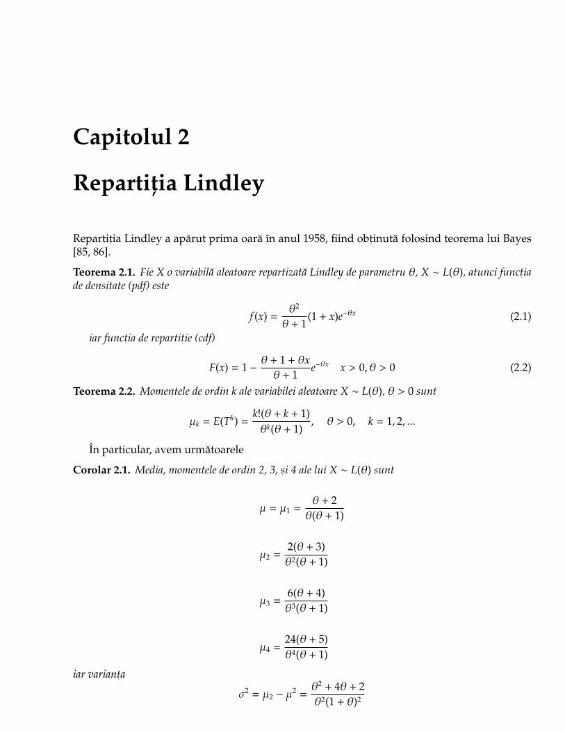
Repartit, ia Lindley a aparut prima oara ın anul 1958, fiind obt, inuta folosind teorema lui Bayes[85, 86].
Teorema 2.1. Fie X o variabila aleatoare repartizata Lindley de parametru θ, X ∼ L(θ), atunci funct, iade densitate (pdf) este
f (x) =θ2
θ + 1(1 + x)e−θx (2.1)
iar funct, ia de repartit, ie (cdf)
F(x) = 1 −θ + 1 + θxθ + 1
e−θx x > 0, θ > 0 (2.2)
Teorema 2.2. Momentele de ordin k ale variabilei aleatoare X ∼ L(θ), θ > 0 sunt
µk = E(Tk) =k!(θ + k + 1)θk(θ + 1)
, θ > 0, k = 1, 2, ...
In particular, avem urmatoarele
Corolar 2.1. Media, momentele de ordin 2, 3, s, i 4 ale lui X ∼ L(θ) sunt
µ = µ1 =θ + 2θ(θ + 1)
µ2 =2(θ + 3)θ2(θ + 1)
µ3 =6(θ + 4)θ3(θ + 1)
µ4 =24(θ + 5)θ4(θ + 1)
iar variant, a
σ2 = µ2 − µ2 =
θ2 + 4θ + 2θ2(1 + θ)2
8
Capitolul 3
Repartit,ia Lindley generalizata
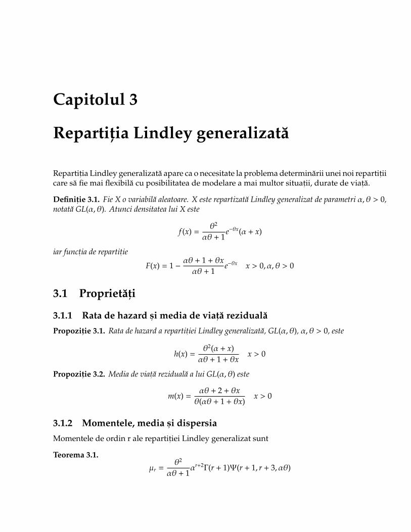
Repartit, ia Lindley generalizata apare ca o necesitate la problema determinarii unei noi repartit, iicare sa fie mai flexibila cu posibilitatea de modelare a mai multor situat, ii, durate de viat, a.
Definit, ie 3.1. Fie X o variabila aleatoare. X este repartizata Lindley generalizat de parametri α, θ > 0,notata GL(α, θ). Atunci densitatea lui X este
f (x) =θ2
αθ + 1e−θx(α + x)
iar funct, ia de repartit, ie
F(x) = 1 −αθ + 1 + θxαθ + 1
e−θx x > 0, α, θ > 0
3.1 Proprietat,i
3.1.1 Rata de hazard s, i media de viat, a reziduala
Propozit, ie 3.1. Rata de hazard a repartit, iei Lindley generalizata, GL(α, θ), α, θ > 0, este
h(x) =θ2(α + x)αθ + 1 + θx
x > 0
Propozit, ie 3.2. Media de viat, a reziduala a lui GL(α, θ) este
m(x) =αθ + 2 + θxθ(αθ + 1 + θx)
x > 0
3.1.2 Momentele, media s, i dispersia
Momentele de ordin r ale repartit, iei Lindley generalizat sunt
Teorema 3.1.
µr =θ2
αθ + 1αr+2Γ(r + 1)Ψ(r + 1, r + 3, αθ)
9
3.1.3 Transformata Laplace-Stieltjes s, i convolut, ii
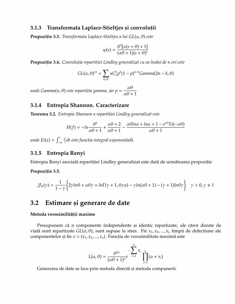
Propozit, ie 3.3. Transformata Laplace-Stieltjes a lui GL(α, θ) este
ϕ(s) =θ2[α(s + θ) + 1](αθ + 1)(s + θ)2
Propozit, ie 3.4. Convolut, ia repartit, iei Lindley generalizat cu ea ınsas, i de n ori este
GL(α, θ)∗n =∑k=0
nCknpk(1 − p)n−kGamma(2n − k, θ)
unde Gamma(n, θ) este repartit, ia gamma, iar p =αθ
αθ + 1
3.1.4 Entropia Shannon. Caracterizare
Teorema 3.2. Entropia Shannon a repartit, iei Lindley generalizat este
H( f ) = −lnθ2
αθ + 1+αθ + 2αθ + 1
−αθlnα + lnα + 1 − eαθEi(−αθ)
αθ + 1
unde Ei(x) =∫ x
−∞
et
t dt este funct, ia integral exponent, iala.
3.1.5 Entropia Renyi
Entropia Renyi asociata repartit, iei Lindley generalizat este data de urmatoarea propozit, ie
Propozit, ie 3.5.
JR(γ) =1
1 − γ
{2γlnθ + αθγ + lnΓ(γ + 1, θγα) − γln(αθ + 1) − (γ + 1)lnθγ
}γ > 0, γ , 1
3.2 Estimare s, i generare de date
Metoda verosimilitat, ii maxime
Presupunem ca n componente independente s, i identic repartizate, ale caror durate deviat, a sunt repartizate GL(α, θ), sunt supuse la stres. Fie x1, x2, ..., xn timpii de defect, iune alecomponentelor s, i fie x = (x1, x2, ..., xn). Funct, ia de verosimilitate maxima este
L(α, θ) =θ2n
(αθ + 1)n e−
n∑i=1
xi n∏i=1
(α + xi)
Generarea de date se face prin metoda directa s, i metoda compunerii.
10
3.3 Statistici de ordine
3.3.1 Momentele statisticilor de ordine
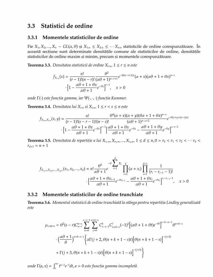
Fie X1,X2, ...,Xn ∼ GL(α, θ) s, i X1:n ≤ X2:n ≤ · · ·Xn:n statisticile de ordine corespunzatoare. Inaceasta sect, iune sunt determinate densitat, ile comune ale statisticilor de ordine, densitat, ilestatisticilor de ordine maxim s, i minim, precum s, i momentele corespunzatoare.
Teorema 3.3. Densitatea statisticii de ordine Xr:n, 1 ≤ r ≤ n este
fXr:n(x) =n!
(r − 1)!(n − r)!θ2
(αθ + 1)n−r+1 e−θ(n−r+1)x(α + x)(αθ + 1 + θx)n−r
·
[1 −
αθ + 1 + θxαθ + 1
e−θx]r−1
, x > 0
unde Γ(·) este funct, ia gamma, iar Ψ(·, ·, ·) funct, ia Kummer.
Teorema 3.4. Densitatea lui Xr:n s, i Xs:n, 1 ≤ r < s ≤ n este
fXr:n,Xs:n(x, y) =n!
(r − 1)!(s − r − 1)!(n − s)!θ4(α + x)(α + y)(θα + 1 + θx)n−s
(αθ + 1)n−s+2 e−θ(x+y+(n−s)x)
·
[1 −
αθ + 1 + θxαθ + 1
e−θx]r−1[αθ + 1 + θx
αθ + 1e−θx−αθ + 1 + θyαθ + 1
e−θy]s−r−1
Teorema 3.5. Densitatea de repartit, ie a lui Xr1:n,Xr2:n, ...,Xrd:n, 1 ≤ d ≤ n, 0 = r0 < r1 < r2 < · · · rd <rd+1 = n + 1
fXr1:n,Xr2:n,...,Xrd :n(x1, x2, ..., xd) = n!θ2
αθ + 1e−θ
d∑i=1
xi d∏i=1
(α + xi)d+1∏i=1
1(ri − ri−1 − 1)!
·
[αθ + 1 + θxi−1
αθ + 1e−θxi−1 −
αθ + 1 + θxi
αθ + 1e−θxi
]ri−ri−1−1, x > 0
3.3.2 Momentele statisticilor de ordine trunchiate
Teorema 3.6. Momentul statisticii de ordine trunchiata la stanga pentru repartit, ia Lindley generalizataeste
µs:n|r:n = θ2(s − r)Cn−sn−r
s−r−1∑k=0
n+k−s∑j=0
Cks−r−1C j
n+k−s(−1)k[(αθ + 1 + θt)e−θt
]s−k−n−1θn+k−s
·
(αθ + 1θ
)n+k−s− j{αΓ( j + 2, θ(n + k + 1 − s)t)
[θ(n + k + 1 − s)
]−( j+2)
+ Γ( j + 3, θ(n + k + 1 − s)t)[θ(n + k + 1 − s)
]−( j+3)}
unde Γ(a, x) =∫∞
xta−1e−tdt, a > 0 este funct, ia gamma incompleta.
11
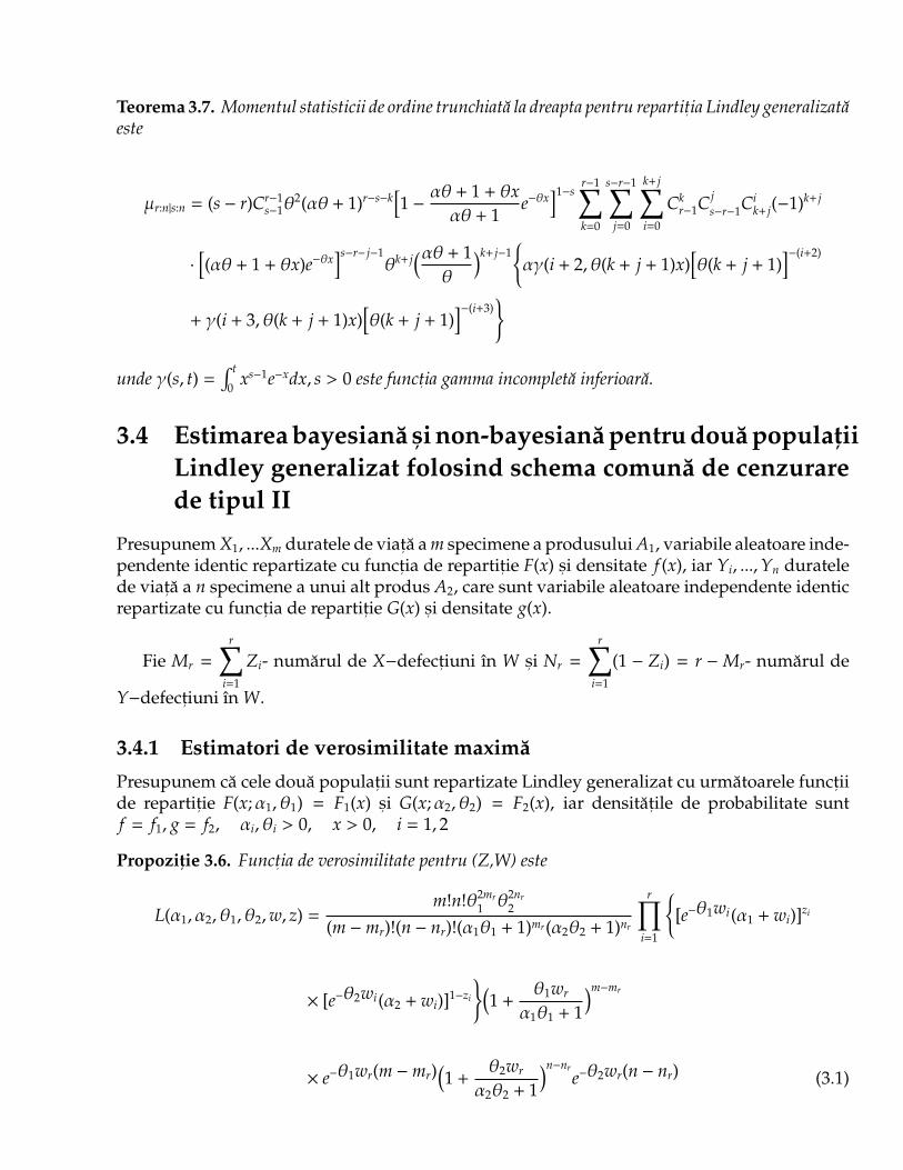
Teorema 3.7. Momentul statisticii de ordine trunchiata la dreapta pentru repartit, ia Lindley generalizataeste
µr:n|s:n = (s − r)Cr−1s−1θ
2(αθ + 1)r−s−k[1 −
αθ + 1 + θxαθ + 1
e−θx]1−s
r−1∑k=0
s−r−1∑j=0
k+ j∑i=0
Ckr−1C j
s−r−1Cik+ j(−1)k+ j
·
[(αθ + 1 + θx)e−θx
]s−r− j−1θk+ j
(αθ + 1θ
)k+ j−1{αγ(i + 2, θ(k + j + 1)x)
[θ(k + j + 1)
]−(i+2)
+ γ(i + 3, θ(k + j + 1)x)[θ(k + j + 1)
]−(i+3)}
unde γ(s, t) =∫ t
0xs−1e−xdx, s > 0 este funct, ia gamma incompleta inferioara.
3.4 Estimarea bayesiana s, i non-bayesiana pentru doua populat,iiLindley generalizat folosind schema comuna de cenzurarede tipul II
Presupunem X1, ...Xm duratele de viat, a a m specimene a produsului A1, variabile aleatoare inde-pendente identic repartizate cu funct, ia de repartit, ie F(x) s, i densitate f (x), iar Yi, ...,Yn duratelede viat, a a n specimene a unui alt produs A2, care sunt variabile aleatoare independente identicrepartizate cu funct, ia de repartit, ie G(x) s, i densitate g(x).
Fie Mr =
r∑i=1
Zi- numarul de X−defect, iuni ın W s, i Nr =
r∑i=1
(1 − Zi) = r −Mr- numarul de
Y−defect, iuni ın W.
3.4.1 Estimatori de verosimilitate maxima
Presupunem ca cele doua populat, ii sunt repartizate Lindley generalizat cu urmatoarele funct, iide repartit, ie F(x;α1, θ1) = F1(x) s, i G(x;α2, θ2) = F2(x), iar densitat, ile de probabilitate suntf = f1, g = f2, αi, θi > 0, x > 0, i = 1, 2
Propozit, ie 3.6. Funct, ia de verosimilitate pentru (Z,W) este
L(α1, α2, θ1, θ2,w, z) =m!n!θ2mr
1 θ2nr2
(m −mr)!(n − nr)!(α1θ1 + 1)mr(α2θ2 + 1)nr
r∏i=1
{[e−θ1wi(α1 + wi)]zi
× [e−θ2wi(α2 + wi)]1−zi
}(1 +
θ1wr
α1θ1 + 1
)m−mr
× e−θ1wr(m −mr)(1 +
θ2wr
α2θ2 + 1
)n−nre−θ2wr(n − nr) (3.1)
12
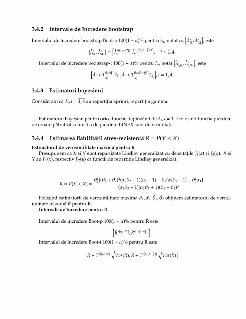
3.4.2 Intervale de ıncredere bootstrap
Intervalul de ıncredere bootstrap Boot-p 100(1 − α)% pentru λi, notat cu[λ∗iL, λ
∗
iU
], este
[λ∗iL, λ∗
iU] =[λ∗([r0α/2])
i , λ∗([r0(1− α2 )])i
], i = 1, 4
Intervalul de ıncredere bootstrap-t 100(1 − α)% pentru λi, notat[λ∗i,tL, λ
∗
i,tU
], este[
λi + T([r0α2 ])
λ∗isλi, λi + T([r0(1− α2 )])
λ∗isλi
], i = 1, 4
3.4.3 Estimatori bayesieni
Consideram ca λi, i = 1, 4 au repartit, ia apriori, repartit, ia gamma.
Estimatorul bayesian pentru orice funct, ie depinzand de λi, i = 1, 4 folosind funct, ia pierderede eroare patratica s, i funct, ia de pierdere LINEX sunt determintat, i.
3.4.4 Estimarea fiabilitat, ii stres-rezistent, a R = P(Y < X)
Estimatorul de verosimilitate maxima pentru RPresupunem ca X s, i Y sunt repartizate Lindley generalizat cu densitat, ile f1(x) s, i f2(y). X s, i
Y au F1(x), respectiv F2(y) ca funct, ii de repartit, ie Lindley generalizat.
R = P(Y < X) =θ2
1[(θ1 + θ2)2(α2θ2 + 1)(α1 − 1) − θ2(α1θ1 + 1) − θ22α1]
(α2θ2 + 1)(α1θ1 + 1)(θ1 + θ2)3
Folosind estimatorii de verosimilitate maxima α1, α2, θ1, θ2 obt, inem estimatorul de verosi-militate maxima R pentru R.
Intervale de ıncredere pentru R
Intervalul de ıncredere Boot-p 100(1 − α)% pentru R este[R∗[r0α/2], R∗[r0(1− α2 )]
]Intervalul de ıncredere Boot-t 100(1 − α)% pentru R este[
R + T∗[r0α/2]√
Var(R), R + T∗[r0(1− α2 )]√
Var(R)]
13
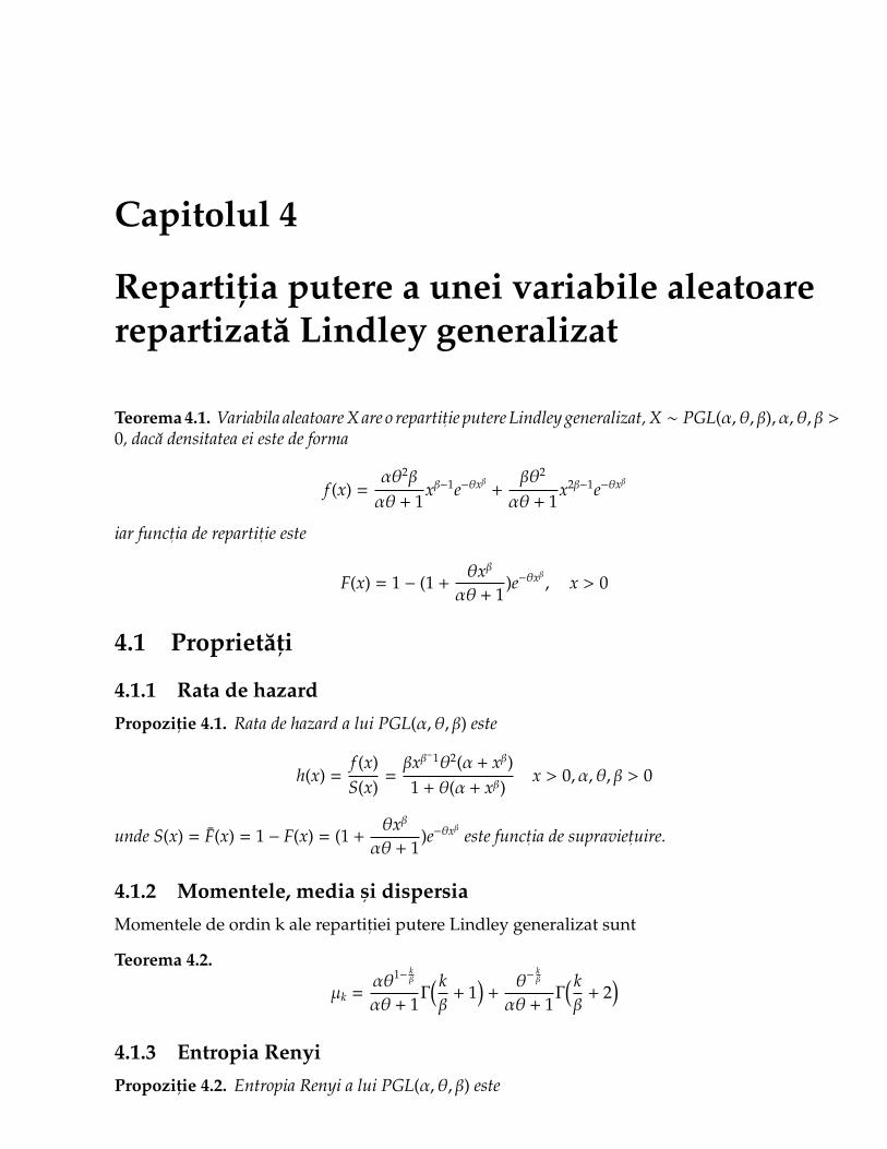
Capitolul 4
Repartit,ia putere a unei variabile aleatoarerepartizata Lindley generalizat
Teorema 4.1. Variabila aleatoare X are o repartit, ie putere Lindley generalizat, X ∼ PGL(α, θ, β), α, θ, β >0, daca densitatea ei este de forma
f (x) =αθ2β
αθ + 1xβ−1e−θxβ +
βθ2
αθ + 1x2β−1e−θxβ
iar funct, ia de repartit, ie este
F(x) = 1 − (1 +θxβ
αθ + 1)e−θxβ , x > 0
4.1 Proprietat,i
4.1.1 Rata de hazard
Propozit, ie 4.1. Rata de hazard a lui PGL(α, θ, β) este
h(x) =f (x)S(x)
=βxβ−1θ2(α + xβ)1 + θ(α + xβ)
x > 0, α, θ, β > 0
unde S(x) = F(x) = 1 − F(x) = (1 +θxβ
αθ + 1)e−θxβ este funct, ia de supraviet, uire.
4.1.2 Momentele, media s, i dispersia
Momentele de ordin k ale repartit, iei putere Lindley generalizat sunt
Teorema 4.2.
µk =αθ1− k
β
αθ + 1Γ(kβ
+ 1)
+θ−
kβ
αθ + 1Γ(kβ
+ 2)
4.1.3 Entropia Renyi
Propozit, ie 4.2. Entropia Renyi a lui PGL(α, θ, β) este
14
JR(γ) =1
1 − γln
{αγθ
γ(β + 1) − 1β βγ−1
(αθ + 1)γγ
γ(β − 1) + 1β
Γ(γ(β − 1) + 1
β
)+
βγ−1
(αθ + 1)γθ
γ − 1β
γ
γ(2β − 1) + 1β
· Γ(γ(2β − 1) + 1
β
)}, γ > 0, γ , 1, iar pentru γ < 1, β > 1 −
1γ
4.2 Generarea de date
Generarea de date pentru repartit, ia putere Lindley generalizat se poate face folosind metodadirecta.
4.3 Statistici de ordine
Teorema 4.3. Repartit, iile asimptotice ale lui X1:n s, i Xn:n sunt
limn→∞
P{
X1:n − an
bn≤ x
}= 1 − e−xβ (4.1)
limn→∞
P{
Xn:n − cn
dn≤ x
}= exp
[− exp(−x)
](4.2)
unde an = 0, bn = F−1(1/n), cn = F−1(1−1/n), dn = 1/n f (cn) s, i F(x)=1-S(x) este funct, ia de repartit, iea lui PGL(α, θ, β)
4.4 Estimatori de verosimilitate maxima
Presupunem ca n componente independente s, i identic repartizate, ale caror durate de viat, asunt repartizate PGL(α, θ, β), sunt supuse la stres. Fie x1, x2, ..., xn timpii de defect, iune alecomponentelor s, i fie x = (x1, x2, ..., xn). Funct, ia de verosimilitate maxima este
L(α, θ, β) = βn( n∏
i=1
xβ−1i
) θ2n
(1 + αθ)n
n∏i=1
(α + xβi )e−θ∑n
i=1 xβi
15
Capitolul 5
Repartit,ii mixate ale duratelor de viat, a
5.1 Repartit,ia Lindley generalizat Poisson Max
Teorema 5.1. Fie X ∼ Lindley generalizat Poisson Max(α, θ, λ). Atunci densitatea de repartit, ie a luiX este
f (x) =λθ2e−θx(x + α)
(αθ + 1)(eλ − 1)eλ[1− αθ+1+θx
αθ+1 e−θx]
iar funct, ia de repartit, ie
F(x) =eλ[1− αθ+1+θx
αθ+1 e−θx]− 1
eλ − 1, x > 0, α, θ, λ > 0
5.1.1 Proprietat, i
Fie X ∼ Lindley generalizat Poisson Max(α, θ, λ), α, θ, λ > 0.
Propozit, ie 5.1. Rata de hazard a lui X ∼ LindleyGeneralizatPoissonMax(α, θ, λ) este
h(y) =λθ2e−θy(y + α)
αθ + 1eλ[1− αθ+1+θy
αθ+1 e−θy]
eλ − eλ[1− αθ+1+θyαθ+1 e−θy]
Propozit, ie 5.2. Rata de hazard h(x) este IFR pe intervalul (0, 1θ − α), cu 1
θ − α > 0.
Teorema 5.2. Momentele de ordin r ≥ 1 sunt
E(Xr) =θ2
e−λ − 1
∑k≥1
(−λ)k
(k − 1)!(αθ + 1)k
{θk−1α
(αθ + 1θ
)r+kΓ(r + 1)Ψ(r + 1, r + k + 1, k(αθ + 1))
+ θk−1(αθ + 1
θ
)r+k+1Γ(r + 2)Ψ(r + 2, r + k + 2, k(αθ + 1))
}unde Ψ(a, b; u) = 1
Γ(a)
∫∞
0ta−1(1 + t)b−a−1e−utdt este funct, ia Kummer, iar Γ(s) =
∫∞
0xs−1e−xdx
Propozit, ie 5.3. Transformata Laplace Stieltjes a repartit, iei Lindley generalizat Poisson Max este
ϕ(s) =∑k≥1
λkθ2
(αθ + 1)k
e−λ
1 − e−λ(−θ)k−1
(k − 1)!αk+1Γ(k)Ψ(k, k + 2, α(s + θk))
16

5.1.2 Entropia Shannon. Caracterizare
Teorema 5.3. Entropia Shannon a repartit, iei Lindley generalizat Poisson Max este
H( f ) = −lnλθ2
(αθ + 1)(eλ − 1)+
θ3
e−λ − 1
∑k≥1
(−λ)k
(k − 1)!(αθ + 1)k
{θk−1α
(αθ + 1θ
)k+1Ψ(2, k + 2, k(αθ + 1))
+ θk−1(αθ + 1
θ
)k+22Ψ(3, k + 3, k(αθ + 1))
}−
∑k≥1
k−1∑i=0
i∑j=0
Cik−1(−1)iC j
iθ j+2λk
(αθ + 1) j+1(eλ − 1)(k − 1)!
{α j+2 π
( j + 2)sin(( j + 2)π)
· 1F1( j + 2, j + 3, αθ(i + 1)) − Γ( j + 2)[θ(i + 1)]−( j+2)
[[ln[θ(i + 1)] −Ψ( j + 2)
]+αθ(i + 1)
j + 1 2F2(1, 1; 2,− j, αθ(i + 1))]
+ α j+2 π( j + 1)sin(( j + 1)π)
· 1F1( j + 1, j + 2, αθ(i + 1)) − Γ( j + 1)[θ(i + 1)]−( j+1)
[[ln[θ(i + 1)] −Ψ( j + 1)
]+αθ(i + 1)
j 2F2(1, 1; 2, 1 − j, αθ(i + 1))]}
−
∑k≥1
k∑i=0
Cik(−1)i λk+1θi+2
(αθ + 1)i+1(eλ − 1)(k − 1)!
[(αθ + 1θ
)i+2Ψ(2, i + 3, (i + 1(αθ + 1)))
+ α(αθ + 1
θ
)i+1Ψ(1, i + 2, (i + 1(αθ + 1)))
]unde
1F1(a; b; z) =
∞∑k=0
(a)kzk
(b)kk!este funct, ia hipergeometrica confluenta
pFq(a1, ..., ap; b1, ..., bq; z) =
∞∑n=0
(a1)n...(ap)n
(b1)n...(bq)n
zn
n!
funct, ia hipergeometrica generalizata
cu (a)n = a(a + 1)(a + 2)...(a + n − 1),n ≥ 1, (a)0 = 1, iar
Ψ(z) = [lnΓ(x)]′
=Γ(x)′
Γ(x)funct, ia psi
Propozit, ie 5.4. Entropia Renyi a repartit, iei Lindley generalizat Poisson Max este
JR(γ) =1
1 − γln
{λγθ2γe−γλ
(1 − e−λ)γ(αθ + 1)λ∑k≥1
k−1∑i=0
γ∑j=0
Cik−1C j
γαγ− j(−1)i
·(λγ)k−1θi
(k − 1)!(αθ + 1)i
(αθ + 1θ
)i+ j+1Γ( j + 1)Ψ( j + 1, j + i + 2, (γ + i)(αθ + 1))
}, γ > 0, γ , 1
17
5.1.3 Generarea de date
Generarea de date se face prin metoda inversa, metoda respingerii s, i metoda compunerii.
5.2 Repartit,ia Lindley generalizat Poisson Min
Teorema 5.4. Fie X ∼ Lindley Generalizat Poisson Min(α, θ,n). Atunci densitatea de repartit, ie avariabilei aleatoare Lindley generalizat Poisson Min este
f (x) =λθ2(α + x)αθ + 1
e−θx 1eλ − 1
eλ
[αθ + 1 + θxαθ + 1
e−θx]
iar funct, ia de repartit, ie
F(x) =1
eλ − 1
[eλ − e
λαθ + 1 + θxαθ + 1
e−θx], x > 0, α, θ, λ > 0
5.2.1 Proprietat, i
Fie X ∼ Lindley generalizat Poisson Min(α, θ, λ), α, θ, λ > 0.
Propozit, ie 5.5. Rata de hazard a lui X este
h(x) =λθ2(α + x)e−θx
αθ + 1eλ
αθ+1+θxαθ+1 e−θx
eλ αθ+1+θxαθ+1 e−θx
− 1
Teorema 5.5. Momentele de ordin r ale repartit, iei sunt
E(Xr) =∑k≥1
θ2
(αθ + 1)k
e−λ
1 − e−λλk
(k − 1)!
{αθk−1
(αθ + 1θ
)r+kΓ(r + 1)Ψ(r + 1, r + k + 1, k(αθ + 1))
+ θk−1(αθ + 1
θ
)r+k+1Γ(r + 2)Ψ(r + 2, r + k + 2, k(αθ + 1))
}unde Γ(s) =
∫∞
0xs−1e−xdx, s > 0 este funct, ia gamma, iar Ψ(·, ·, ·) funct, ia Kummer.
Transformata Laplace Stieltjes
Propozit, ie 5.6. Transformata Laplace Stieltjes a repartit, iei Lindley generalizat Poisson Min este
ϕ(s) =∑k≥1
λk
(αθ + 1)k
e−λ
1 − e−λθk+1
(k − 1)!
{α(αθ + 1
θ
)kΨ(1, k + 1, (s + θk)
αθ + 1θ
)
+(αθ + 1
θ
)k+1Ψ(2, k + 2, (s + θk)
αθ + 1θ
)}
18
5.2.2 Entropia Shannon. Caracterizare
Teorema 5.6. Entropia Shannon a repartit, iei Lindley generalizat Poisson Min este
H( f ) = −lnλθ2
(αθ + 1)(eλ − 1)+
∑k≥1
θ3
(αθ + 1)k
e−λ
1 − e−λλk
(k − 1)!
{αθk−1
(αθ + 1θ
)1+kΨ(2, k + 2, k(αθ + 1))
+ θk−1(αθ + 1
θ
)k+22Ψ(3, k + 3, k(αθ + 1))
}−
∑k≥1
λk+1θk+2
(αθ + 1)k+1(eλ − 1)(k − 1)!
[α(αθ + 1
θ
)k+1Ψ(1, k + 2, (k + 1)(αθ + 1))
+(αθ + 1
θ
)k+2Ψ(2, k + 3, (k + 1)(αθ + 1))
]−
∑k≥1
k−1∑i=0
Cik−1
θi+2λk
(αθ + 1)i+1(eλ − 1)(k − 1)!
{αi+2 π
(i + 1)sin((i + 1)π)
· 1F1(i + 1, i + 2, αθk) − Γ(i + 1)[θk]−(i+1)
[[ln[θk] −Ψ(i + 1)
]+αθk
i 2F2(1, 1; 2, 1 − i, αθk]
+ αi+2 π(i + 2)sin((i + 2)π) 1F1(i + 2, i + 3, αθk) − Γ(i + 2)[θk]−(i+2)
[[ln[θk] −Ψ(i + 2)
]+αθki + 1 2F2(1, 1; 2,−i, αθk
]}Entropia Renyi
Propozit, ie 5.7. Entropia Renyi pentru repartit, ia Lindley generalizat Poisson Min este
JR(γ) =1
1 − γln
{λγθ2γ
(αθ + 1)γ( 1eλ − 1
)γ∑k≥1
γ∑i=0
Ciγα
γ−i (λγ)k−1θk−1
(αθ + 1)k−1(k − 1)!
·
(αθ + 1θ
)i+kΓ(i + 1)Ψ(i + 1, i + k + 1, (αθ + 1)(γ + k − 1))
}, γ > 0, γ , 1
unde Γ(·) este funct, ia gamma, iar Ψ(·, ·, ·) funct, ia Kummer.
5.2.3 Generarea de date
Generarea de date se face prin metoda inversa, metoda respingerii s, i metoda compunerii.
5.3 Repartit,ia Lindley generalizat Binomial Max
Teorema 5.7. Fie X ∼ Lindley generalizat Binomial Max(α, θ,n, p). Atunci densitatea de repartit, ie alui X este
f (x) =θ2(α + x)αθ + 1
e−θx np1 − qn
[1 − p
αθ + 1 + θxαθ + 1
e−θx]n−1
19
iar funct, ia de repartit, ie
F(x) =1
1 − qn
{[1 − p
αθ + 1 + θxαθ + 1
e−θx]n− qn
}, x > 0, θ, α, p > 0
5.3.1 Proprietat, i
Fie X ∼ Lindley generalizat Binomial Max(α, θ,n, p), α, θ, p > 0.
Propozit, ie 5.8. Rata de hazard a repartit, iei Lindley generalizat Binomial Max este
h(y) =θ2e−θy(α + y)np
[1 − pαθ+1+θy
αθ+1 e−θy]n−1
(αθ + 1){1 −
[1 − pαθ+1+θy
αθ+1 e−θy]n}
Lema 5.1. Fie H(a, b, c, d, δ, p) =∫∞
0xc(d + x)
[1 − p1+bd+bx
1+bd e−bx]a−1
e−δxdx, 1 + bd > 0.
Avem ca
H(a, b, c, d, δ, p) =
∞∑i=0
i∑j=0
j+1∑k=0
Cia−1C j
i Ckj+1
(−1)ipi
(1 + bd)i bjd j+1−k Γ(c + k + 1)
(bi + j)c+k+1
Teorema 5.8. Momentele de ordin r ale lui X sunt
E(Xr) =θ2np
(αθ + 1)(1 − qn)H(n − 1, θ, r, α, θ, p)
Propozit, ie 5.9. Transformata Laplace Stieltjes a repartit, iei Lindley generalizat Binomial Max este
ϕ(s) =npθ2
(αθ + 1)(1 − qn)
n−1∑k=0
Ckn−1
(−1)k
(αθ + 1)kθk
{α(αθ + 1
θ
)k+1Ψ(1, k + 2,
αθ + 1θ
[s + θ(k + 1)])
+(αθ + 1
θ
)k+2Ψ(2, k + 3,
αθ + 1θ
[s + θ(k + 1)])}
unde Γ(·) este funct, ia gamma, iar Ψ(·, ·, ·) este funct, ia Kummer.
5.3.2 Entropia Shannon. Caracterizare
Teorema 5.9. Entropia Shannon a repartit, iei Lindley generalizat Binomial Max este
20
H( f ) = −lnθ2np
(αθ + 1)(1 − qn)+
θ3np(αθ + 1)(1 − qn)
H(n − 1, θ, 1, α, θ, p)
−
n−1∑k=0
k∑i=0
Ckn−1(−1)kCi
k
θi+2npk+1
(αθ + 1)i+1(1 − qn)
{αi+2 π
(i + 2)sin((i + 2)π)
· 1F1(i + 2, i + 3, αθ(k + 1)) − Γ(i + 2)[θ(k + 1)]−(i+2)
[[ln[θ(k + 1)] −Ψ(i + 2)
]+αθ(k + 1)
i + 1 2F2(1, 1; 2,−i, αθ(k + 1)]
+ αi+2 π(i + 1)sin((i + 1)π) 1F1(i + 1, i + 2, αθ(k + 1))
− Γ(i + 1)[θ(k + 1)]−(i+1)
[[ln[θ(k + 1)] −Ψ(i + 1)
]+αθ(k + 1)
i 2F2(1, 1; 2, 1 − i, αθ(k + 1)]}
+ (n − 1)(1n
+qn
1 − qn ln(q))
Propozit, ie 5.10. Entropia repartit, iei Lindley generalizat Binomial Max este
JR(γ) =1
1 − γln
{( np1 − qn
)γ n−1∑k=0
γ∑i=0
Ckn−1Cγ
i αγ−i(−1)k (αθ + 1)i+1−γpk
θi+1−2γ
· Γ(i + 1)Ψ(i + 1, i + k + 2, (αθ + 1)(γ + k))}
unde Γ(s) =∫∞
0xs−1e−xdx este funct, ia gamma, iar Ψ(·, ·, ·) funct, ia Kummer.
5.3.3 Generarea de date
Generarea de date se face prin metoda inversa, metoda respingerii s, i metoda compunerii.
5.4 Repartit,ia Lindley generalizat Binomial Min
Teorema 5.10. Fie X ∼ Lindley generalizat Binomial Min. Atunci funct, ia de repartit, ie a lui X este
F(x) = 1 −1
1 − qn
{[q + p
αθ + 1 + θxαθ + 1
e−θx
]n
− qn
}(5.1)
iar densitatea de repartit, ie
f (x) =np
1 − qn
[q + p
θα + 1 + θxαθ + 1
e−θx]n−1
fGL(α,θ)(x), x > 0, α, θ, p > 0 (5.2)
5.4.1 Proprietat, i
Fie X ∼ Lindley generalizat Binomial Min(α, θ,n, p).
21
Propozit, ie 5.11. Rata de hazard a lui X este
h(t) =
np[q + pθα+1+θx
αθ+1 e−θx]n−1
fGL(α,θ)(t)[q + pθα+1+θx
αθ+1 e−θx]n
− qn
Teorema 5.11. Momentele de ordin r ale repartit, iei Lindley generalizat Binomial Min sunt
E(Xr) =npθ2
(1 − qn)(αθ + 1)
n−1∑k=0
pk qn−1−k
(αθ + 1)kCk
n−1
{αθk
(αθ + 1θ
)r+k+1Γ(r + 1)
·Ψ(r + 1, r + 2 + k, θ(k + 1)αθ + 1θ
) + θk(αθ + 1
θ
)r+2+kΓ(r + 2)Ψ(r + 2, r + 3 + k, θ(k + 1)
αθ + 1θ
)}
unde Ψ(a, b; u) este funct, ia Kummer.
Propozit, ie 5.12. Transformata Laplace-Stieltjes pentru repartit, ia Lindley generalizat Binomial Min areurmatoarea forma
ϕ(s) =npθ2
(1 − qn)(αθ + 1)
n−1∑k=0
pk qn−1−k
(αθ + 1)kCk
n−1
{θkα
(αθ + 1θ
)k+1Ψ(1, k + 2,
αθ + 1θ
[s + θ(k + 1)])
+ θk(αθ + 1
θ
)k+2Ψ(2, k + 3,
αθ + 1θ
[s + θ(k + 1)])}
unde Γ(·)este funct, ia gamma, iar Ψ(·, ·, ·) este funct, ia Kummer
5.4.2 Entropia Shannon. Caracterizare
Teorema 5.12. Entropia Shannon a repartit, ei Lindley generalizat Binomial Min este
H( f ) = −lnnpθ2
(αθ + 1)(1 − qn)+
npθ3
(1 − qn)(αθ + 1)
n−1∑k=0
pk qn−1−k
(αθ + 1)kCk
n−1
[αθk
(αθ + 1θ
)k+2
·Ψ(2, k + 3, θ(k + 1)αθ + 1θ
) + θk(αθ + 1
θ
)k+32Ψ(3, k + 4, θ(k + 1)
αθ + 1θ
)]
−
n−1∑k=0
k∑i=0
Ckn−1Ci
k
θi+2npk+1qn−1−k
(αθ + 1)i+1(1 − qn)
{αi+2 π
(i + 2)sin((i + 2)π)
· 1F1(i + 2, i + 3, αθk) − Γ(i + 2)[θk]−(i+2)
[[ln[θk] −Ψ(i + 2)
]+αθki + 12F2(1, 1; 2,−i, αθk)
]+ αi+2 π
(i + 1)sin((i + 1)π)1F1(i + 1, i + 2, αθk) − Γ(i + 1)[θk]−(i+1)
[[ln[θk] −Ψ(i + 1)
]+αθk
i 2F2(1, 1; 2, 1 − i, αθk)]}
+(1n
+qn
1 − qn ln(q))
22
Propozit, ie 5.13. Entropia Renyi a lui X este
JR(γ) =1
1 − γln
{( np1 − qn
)γ (n−1)γ∑k=0
γ∑i=0
Ck(n−1)γCi
γ
θ2γ−i−1pkαγ−iq(n−1)γ−k
(αθ + 1)γ−i−1
· Γ(i + 1)Ψ(i + 1, i + k + 1, (k + γ)(αθ + 1))}, γ > 0, γ , 1
unde Γ(·) este funct, ia gamma, iar ψ(·, ·, ·) funct, ia Kummer.
5.4.3 Generarea de date
Generarea de date se face prin metoda inversa, metoda respingerii s, i metoda compunerii.
5.5 Repartit,ia Lindley generalizat Geometric Max
Teorema 5.13. Fie X ∼ Lindley generalizat Geometric Max. Atunci densitatea lui X este
f (x) =pθ2(α + x)e−θx
αθ + 1
[1 − (1 − p)
(1 −
αθ + 1 + θxαθ + 1
e−θx)]−2
iar funct, ia de repartit, ie
F(x) =p
1 − p
[1
1 − (1 − p)(1 − αθ+1+θx
αθ+1 e−θx) − 1
], x > 0, α, θ, p > 0
5.5.1 Proprietat, ii
Fie X ∼ Lindley generalizat Geometric Max(α, θ, p), α, θ, p > 0.
Propozit, ie 5.14. Rata de hazard a lui X este
h(x) =pθ2(α + x)αθ + 1 + θx
[1
1 − (1 − p)(1 − αθ+1+θx
αθ+1 e−θx)]
Propozit, ie 5.15. Rata de hazard h(x) este IFR.
Teorema 5.14. Momentele de ordin r ale repartit, iei Lindley generalizat Geometric Max sunt
E(Xr) =∑k≥1
kpθ2(1 − p)k−1
(αθ + 1)k(−θ)k−1αk+r+1Γ(k + r)Ψ(k + r, k + r + 2, αkθ)
unde Γ(·) este funct, ia gamma, iar Ψ(·, ·, ·) funct, ia Kummer.
Propozit, ie 5.16. Transformata Laplace Stieltjes a repartit, iei Lindley generalizat Geometric Max este
ϕ(s) =∑k≥1
kpθ2(1 − p)k−1(−θ)k−1
(αθ + 1)kαk+1Γ(k)Ψ(k, k + 2, α(θk + s))
23
5.5.2 Entropia Shannon. Caracterizare
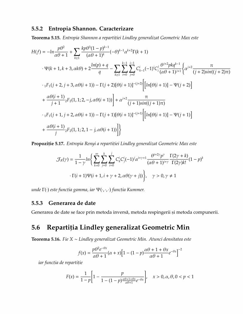
Teorema 5.15. Entropia Shannon a repartit, iei Lindley generalizat Geometric Max este
H( f ) = −lnpθ2
αθ + 1+
∑k≥1
kpθ3(1 − p)k−1
(αθ + 1)k(−θ)k−1αk+2Γ(k + 1)
·Ψ(k + 1, k + 3, αkθ) + 2ln(p) + q
q−
∑k≥1
k−1∑i=0
i−1∑j=0
Cik−1(−1)iC j
i
θ j+2pkqk−1
(αθ + 1) j+1
{α j+2 π
( j + 2)sin(( j + 2)π)
· 1F1( j + 2, j + 3, αθ(i + 1)) − Γ( j + 2)[θ(i + 1)]−( j+2)
[[ln[θ(i + 1)] −Ψ( j + 2)
]+αθ(i + 1)
j + 1 2F2(1, 1; 2,− j, αθ(i + 1))]
+ α j+2 π( j + 1)sin(( j + 1)π)
· 1F1( j + 1, j + 2, αθ(i + 1)) − Γ( j + 1)[θ(i + 1)]−( j+1)
[[ln[θ(i + 1)] −Ψ( j + 1)
]+αθ(i + 1)
j 2F2(1, 1; 2, 1 − j, αθ(i + 1))]}
Propozit, ie 5.17. Entropia Renyi a repartit, iei Lindley generalizat Geometric Max este
JR(γ) =1
1 − γln
{ ∞∑k=0
k∑j=0
j∑i=0
CikC
ij(−1) jαi+γ+1 θi+2γpγ
(αθ + 1)i+γ
Γ(2γ + k)Γ(2γ)k!
(1 − p)k
· Γ(i + 1)Ψ(i + 1, i + γ + 2, αθ(γ + j))}, γ > 0, γ , 1
unde Γ(·) este funct, ia gamma, iar Ψ(·, ·, ·) funct, ia Kummer.
5.5.3 Generarea de date
Generarea de date se face prin metoda inversa, metoda respingerii s, i metoda compunerii.
5.6 Repartit,ia Lindley generalizat Geometric Min
Teorema 5.16. Fie X ∼ Lindley generalizat Geometric Min. Atunci densitatea este
f (x) =pθ2e−θx
αθ + 1(α + x)
[1 − (1 − p)
αθ + 1 + θxαθ + 1
e−θx]−2
iar funct, ia de repartit, ie
F(x) =1
1 − p
[1 −
p1 − (1 − p)αθ+1+θx
αθ+1 e−θx
], x > 0, α, θ, 0 < p < 1
24
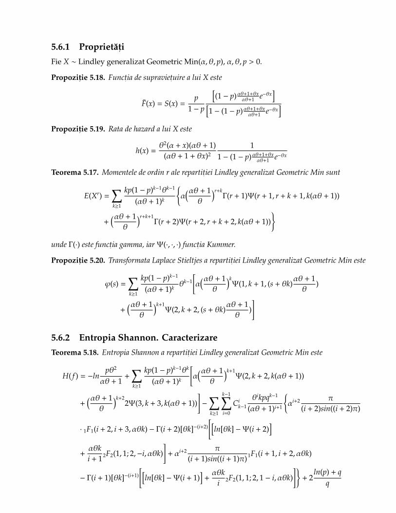
5.6.1 Proprietat, i
Fie X ∼ Lindley generalizat Geometric Min(α, θ, p), α, θ, p > 0.
Propozit, ie 5.18. Funct, ia de supraviet, uire a lui X este
F(x) = S(x) =p
1 − p
[(1 − p)αθ+1+θx
αθ+1 e−θx][
1 − (1 − p)αθ+1+θxαθ+1 e−θx
]Propozit, ie 5.19. Rata de hazard a lui X este
h(x) =θ2(α + x)(αθ + 1)
(αθ + 1 + θx)2
11 − (1 − p)αθ+1+θx
αθ+1 e−θx
Teorema 5.17. Momentele de ordin r ale repartit, iei Lindley generalizat Geometric Min sunt
E(Xr) =∑k≥1
kp(1 − p)k−1θk−1
(αθ + 1)k
{α(αθ + 1
θ
)r+kΓ(r + 1)Ψ(r + 1, r + k + 1, k(αθ + 1))
+(αθ + 1
θ
)r+k+1Γ(r + 2)Ψ(r + 2, r + k + 2, k(αθ + 1))
}unde Γ(·) este funct, ia gamma, iar Ψ(·, ·, ·) funct, ia Kummer.
Propozit, ie 5.20. Transformata Laplace Stieltjes a repartit, iei Lindley generalizat Geometric Min este
ϕ(s) =∑k≥1
kp(1 − p)k−1
(αθ + 1)kθk−1
[α(αθ + 1
θ
)kΨ(1, k + 1, (s + θk)
αθ + 1θ
)
+(αθ + 1
θ
)k+1Ψ(2, k + 2, (s + θk)
αθ + 1θ
)]
5.6.2 Entropia Shannon. Caracterizare
Teorema 5.18. Entropia Shannon a repartit, iei Lindley generalizat Geometric Min este
H( f ) = −lnpθ2
αθ + 1+
∑k≥1
kp(1 − p)k−1θk
(αθ + 1)k
[α(αθ + 1
θ
)k+1Ψ(2, k + 2, k(αθ + 1))
+(αθ + 1
θ
)k+22Ψ(3, k + 3, k(αθ + 1))
]−
∑k≥1
k−1∑i=0
Cik−1
θikpqk−1
(αθ + 1)i+1
{αi+2 π
(i + 2)sin((i + 2)π)
· 1F1(i + 2, i + 3, αθk) − Γ(i + 2)[θk]−(i+2)
[[ln[θk] −Ψ(i + 2)
]+αθki + 12F2(1, 1; 2,−i, αθk)
]+ αi+2 π
(i + 1)sin((i + 1)π) 1F1(i + 1, i + 2, αθk)
− Γ(i + 1)[θk]−(i+1)
[[ln[θk] −Ψ(i + 1)
]+αθk
i 2F2(1, 1; 2, 1 − i, αθk)]}
+ 2ln(p) + q
q
25
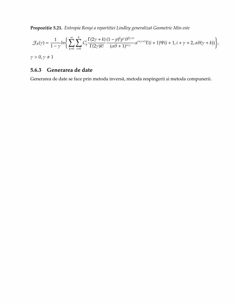
Propozit, ie 5.21. Entropia Renyi a repartit, iei Lindley generalizat Geometric Min este
JR(γ) =1
1 − γln
{ ∞∑k=0
k∑i=0
Cik
Γ(2γ + k)Γ(2γ)k!
(1 − p)kpγθ2γ+i
(αθ + 1)i+γ αi+γ+1Γ(i + 1)Ψ(i + 1, i + γ + 2, αθ(γ + k))},
γ > 0, γ , 1
5.6.3 Generarea de date
Generarea de date se face prin metoda inversa, metoda respingerii s, i metoda compunerii.
26
Capitolul 6
Procese de reınnoire
6.1 Procese de reınnoire
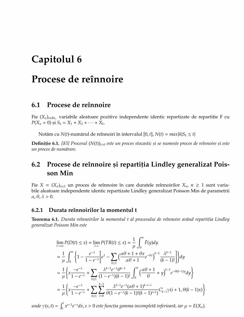
Fie (Xn)n∈N+ variabile aleatoare pozitive independente identic repartizate de repartit, ie F cuP(Xn = 0) s, i Sk = X1 + X2 + · · · + Xk.
Notam cu N(t)-numarul de reınnoiri ın intervalul [0, t], N(t) = max{k|Sk ≤ t}
Definit, ie 6.1. [83] Procesul (N(t))t>0 este un proces stocastic s, i se numes, te proces de reınnoire s, i esteun proces de numarare.
6.2 Procese de reınnoire s, i repartit,ia Lindley generalizat Pois-son Min
Fie X = (Xn)n≥1 un proces de reınnoire ın care duratele reınnoirilor Xn, n ≥ 1 sunt varia-bile aleatoare independente identic repartizate Lindley generalizat Poisson Min de parametriiα, θ, λ > 0.
6.2.1 Durata reınnoirilor la momentul t
Teorema 6.1. Durata reınnoirilor la momentul t al procesului de reınnoire avand repartit, ia Lindleygeneralizat Poisson Min este
limt→∞
P(D(t) ≤ x) = limt→
P(TR(t) ≤ x) =1µ
∫ x
0F(y)dy
=1µ
∫ x
0
{1 −
e−λ
1 − e−λ
[eλ −
∑k≥1
(αθ + 1 + θxαθ + 1
e−θx)k−1 λk−1
(k − 1)!
]}dy
=1µ
{x−e−λ
1 − e−λ+
∑k≥1
λk−1e−λθk−1
(1 − e−λ)(k − 1)!
∫ x
0
(αθ + 1θ
+ y)k−1
e−θ(k−1)ydy}
=1µ
{x−e−λ
1 − e−λ+
∑k≥1
k−1∑i=0
λk−1e−λ(αθ + 1)k−i−i
θ(1 − e−λ(k − 1)!(k − 1)i+1)Ci
k−1γ(i + 1, θ(k − 1)x)}
unde γ(s, t) =∫ t
0xs−1e−xdx, s > 0 este funct, ia gamma incompleta inferioara, iar µ = E(Xn).
27
6.3 Procese de reınnoire s, i repartit,ia Lindley generalizat Bino-mial Min
Fie X = (Xn)n≥1 un proces de reınnoire ın care duratele reınnoirilor Xn, n ≥ 1 sunt variabilealeatoare independente identic repartizate Lindley generalizat Binomial Min de parametriiα, θ, p > 0,n ≥ 1.
6.3.1 Durata reınnoirilor la momentul t
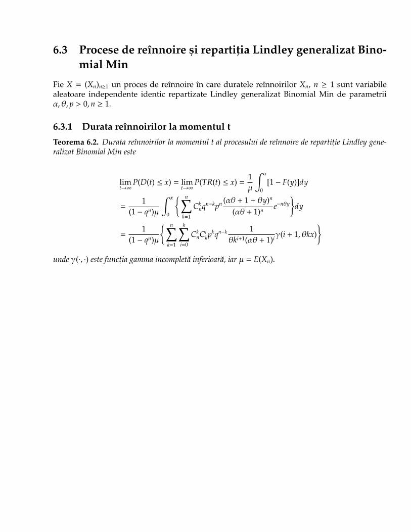
Teorema 6.2. Durata reınnoirilor la momentul t al procesului de reınnoire de repartit, ie Lindley gene-ralizat Binomial Min este
limt→∞
P(D(t) ≤ x) = limt→∞
P(TR(t) ≤ x) =1µ
∫ x
0[1 − F(y)]dy
=1
(1 − qn)µ
∫ x
0
{ n∑k=1
Cknqn−kpn (αθ + 1 + θy)n
(αθ + 1)n e−nθy
}dy
=1
(1 − qn)µ
{ n∑k=1
k∑i=0
CknCi
kpkqn−k 1
θki+1(αθ + 1)iγ(i + 1, θkx)}
unde γ(·, ·) este funct, ia gamma incompleta inferioara, iar µ = E(Xn).
28
Capitolul 7
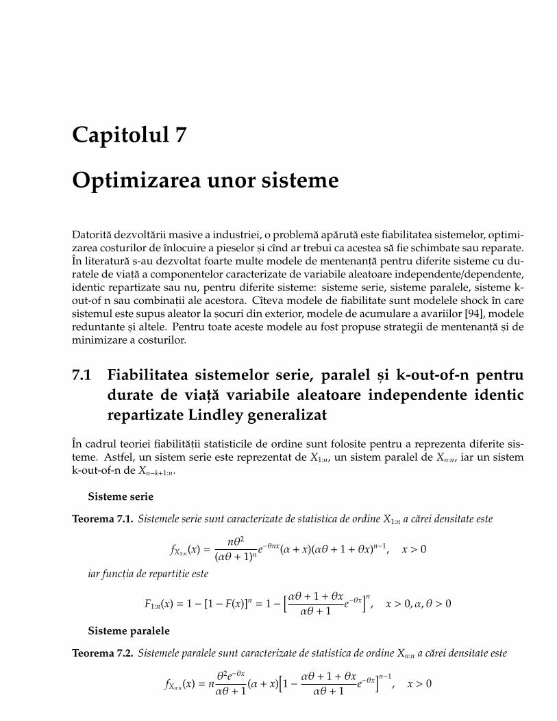
Optimizarea unor sisteme
Datorita dezvoltarii masive a industriei, o problema aparuta este fiabilitatea sistemelor, optimi-zarea costurilor de ınlocuire a pieselor s, i cınd ar trebui ca acestea sa fie schimbate sau reparate.In literatura s-au dezvoltat foarte multe modele de mentenant, a pentru diferite sisteme cu du-ratele de viat, a a componentelor caracterizate de variabile aleatoare independente/dependente,identic repartizate sau nu, pentru diferite sisteme: sisteme serie, sisteme paralele, sisteme k-out-of n sau combinat, ii ale acestora. Cıteva modele de fiabilitate sunt modelele shock ın caresistemul este supus aleator la s, ocuri din exterior, modele de acumulare a avariilor [94], modelereduntante s, i altele. Pentru toate aceste modele au fost propuse strategii de mentenant, a s, i deminimizare a costurilor.
7.1 Fiabilitatea sistemelor serie, paralel s, i k-out-of-n pentrudurate de viat, a variabile aleatoare independente identicrepartizate Lindley generalizat
In cadrul teoriei fiabilitat, ii statisticile de ordine sunt folosite pentru a reprezenta diferite sis-teme. Astfel, un sistem serie este reprezentat de X1:n, un sistem paralel de Xn:n, iar un sistemk-out-of-n de Xn−k+1:n.
Sisteme serie
Teorema 7.1. Sistemele serie sunt caracterizate de statistica de ordine X1:n a carei densitate este
fX1:n(x) =nθ2
(αθ + 1)n e−θnx(α + x)(αθ + 1 + θx)n−1, x > 0
iar funct, ia de repartit, ie este
F1:n(x) = 1 − [1 − F(x)]n = 1 −[αθ + 1 + θx
αθ + 1e−θx
]n, x > 0, α, θ > 0
Sisteme paralele
Teorema 7.2. Sistemele paralele sunt caracterizate de statistica de ordine Xn:n a carei densitate este
fXn:n(x) = nθ2e−θx
αθ + 1(α + x)
[1 −
αθ + 1 + θxαθ + 1
e−θx]n−1
, x > 0
29
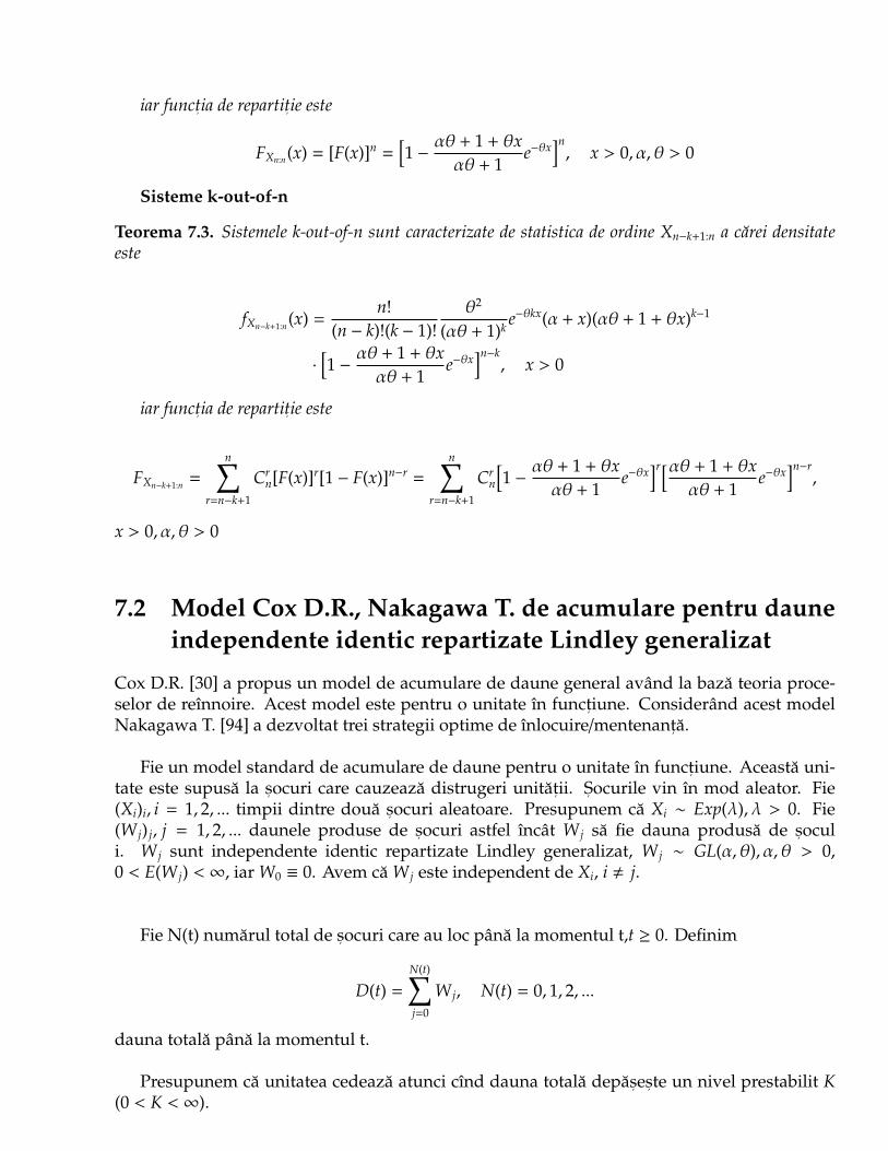
iar funct, ia de repartit, ie este
FXn:n(x) = [F(x)]n =[1 −
αθ + 1 + θxαθ + 1
e−θx]n, x > 0, α, θ > 0
Sisteme k-out-of-n
Teorema 7.3. Sistemele k-out-of-n sunt caracterizate de statistica de ordine Xn−k+1:n a carei densitateeste
fXn−k+1:n(x) =n!
(n − k)!(k − 1)!θ2
(αθ + 1)ke−θkx(α + x)(αθ + 1 + θx)k−1
·
[1 −
αθ + 1 + θxαθ + 1
e−θx]n−k
, x > 0
iar funct, ia de repartit, ie este
FXn−k+1:n =
n∑r=n−k+1
Crn[F(x)]r[1 − F(x)]n−r =
n∑r=n−k+1
Crn
[1 −
αθ + 1 + θxαθ + 1
e−θx]r[αθ + 1 + θx
αθ + 1e−θx
]n−r,
x > 0, α, θ > 0
7.2 Model Cox D.R., Nakagawa T. de acumulare pentru dauneindependente identic repartizate Lindley generalizat
Cox D.R. [30] a propus un model de acumulare de daune general avand la baza teoria proce-selor de reınnoire. Acest model este pentru o unitate ın funct, iune. Considerand acest modelNakagawa T. [94] a dezvoltat trei strategii optime de ınlocuire/mentenant, a.
Fie un model standard de acumulare de daune pentru o unitate ın funct, iune. Aceasta uni-tate este supusa la s, ocuri care cauzeaza distrugeri unitat, ii. S, ocurile vin ın mod aleator. Fie(Xi)i, i = 1, 2, ... timpii dintre doua s, ocuri aleatoare. Presupunem ca Xi ∼ Exp(λ), λ > 0. Fie(W j) j, j = 1, 2, ... daunele produse de s, ocuri astfel ıncat W j sa fie dauna produsa de s, oculi. W j sunt independente identic repartizate Lindley generalizat, W j ∼ GL(α, θ), α, θ > 0,0 < E(W j) < ∞, iar W0 ≡ 0. Avem ca W j este independent de Xi, i , j.
Fie N(t) numarul total de s, ocuri care au loc pana la momentul t,t ≥ 0. Definim
D(t) =
N(t)∑j=0
W j, N(t) = 0, 1, 2, ...
dauna totala pana la momentul t.
Presupunem ca unitatea cedeaza atunci cınd dauna totala depas, es, te un nivel prestabilit K(0 < K < ∞).
30
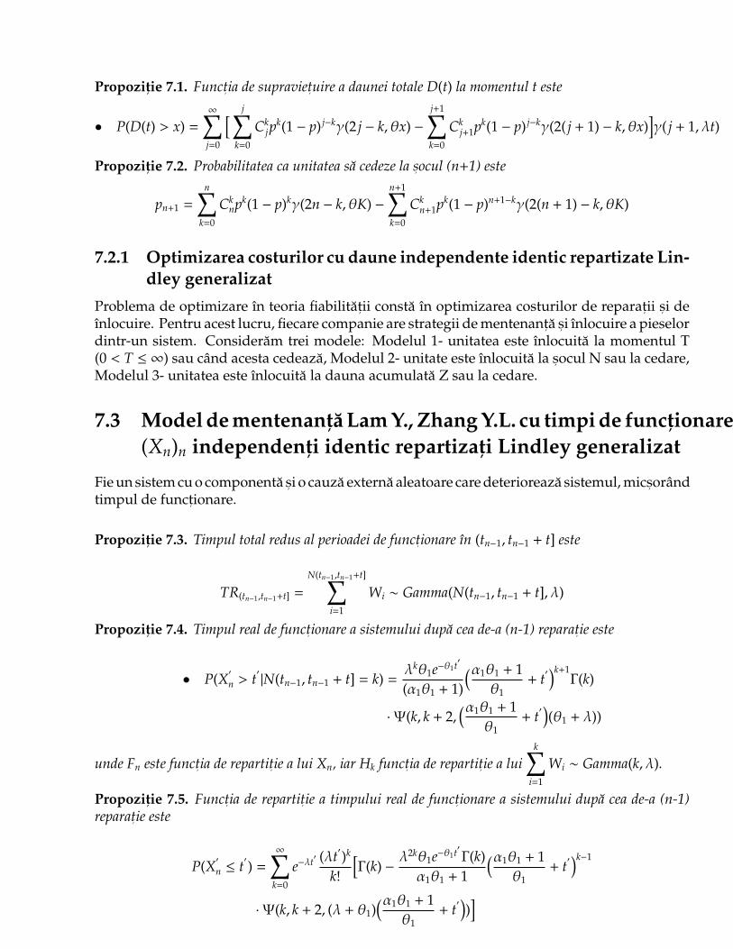
Propozit, ie 7.1. Funct, ia de supraviet, uire a daunei totale D(t) la momentul t este
• P(D(t) > x) =
∞∑j=0
[ j∑k=0
Ckjp
k(1 − p) j−kγ(2 j − k, θx) −j+1∑k=0
Ckj+1pk(1 − p) j−kγ(2( j + 1) − k, θx)
]γ( j + 1, λt)
Propozit, ie 7.2. Probabilitatea ca unitatea sa cedeze la s, ocul (n+1) este
pn+1 =
n∑k=0
Cknpk(1 − p)kγ(2n − k, θK) −
n+1∑k=0
Ckn+1pk(1 − p)n+1−kγ(2(n + 1) − k, θK)
7.2.1 Optimizarea costurilor cu daune independente identic repartizate Lin-dley generalizat
Problema de optimizare ın teoria fiabilitat, ii consta ın optimizarea costurilor de reparat, ii s, i deınlocuire. Pentru acest lucru, fiecare companie are strategii de mentenant, a s, i ınlocuire a pieselordintr-un sistem. Consideram trei modele: Modelul 1- unitatea este ınlocuita la momentul T(0 < T ≤ ∞) sau cand acesta cedeaza, Modelul 2- unitate este ınlocuita la s, ocul N sau la cedare,Modelul 3- unitatea este ınlocuita la dauna acumulata Z sau la cedare.
7.3 Model de mentenant, a Lam Y., Zhang Y.L. cu timpi de funct,ionare(Xn)n independent,i identic repartizat,i Lindley generalizat
Fie un sistem cu o componenta s, i o cauza externa aleatoare care deterioreaza sistemul, mics, orandtimpul de funct, ionare.
Propozit, ie 7.3. Timpul total redus al perioadei de funct, ionare ın (tn−1, tn−1 + t] este
TR(tn−1,tn−1+t] =
N(tn−1,tn−1+t]∑i=1
Wi ∼ Gamma(N(tn−1, tn−1 + t], λ)
Propozit, ie 7.4. Timpul real de funct, ionare a sistemului dupa cea de-a (n-1) reparat, ie este
• P(X′
n > t′
|N(tn−1, tn−1 + t] = k) =λkθ1e−θ1t
′
(α1θ1 + 1)
(α1θ1 + 1θ1
+ t′)k+1
Γ(k)
·Ψ(k, k + 2,(α1θ1 + 1
θ1+ t
′)(θ1 + λ))
unde Fn este funct, ia de repartit, ie a lui Xn, iar Hk funct, ia de repartit, ie a luik∑
i=1
Wi ∼ Gamma(k, λ).
Propozit, ie 7.5. Funct, ia de repartit, ie a timpului real de funct, ionare a sistemului dupa cea de-a (n-1)reparat, ie este
P(X′
n ≤ t′
) =
∞∑k=0
e−λt′ (λt′)k
k!
[Γ(k) −
λ2kθ1e−θ1t′
Γ(k)α1θ1 + 1
(α1θ1 + 1θ1
+ t′)k−1
·Ψ(k, k + 2, (λ + θ1)(α1θ1 + 1
θ1+ t
′))]
31
Fie
h(N) =
(c + r)α2θ2 + 2
θ2(α2θ2 + 1)
( N∑i=1
µ′
i − µ′
N+1(N − 1) + δ)
(R + cpδ + rδ)(µ′N+1 +α2θ2 + 2
θ2(α2θ2 + 1))
Teorema 7.4. Strategia de mentenant, a optima N∗ este determinata astfel
N∗ = min{N|h(N) ≥ 1}
N∗ este unic daca s, i numai daca h(N∗) > 1.
7.4 Ret,elele Ad-Hoc ZRP Ben Liang, Zgymunt J. Haas pentrudurate Lindley generalizat ale legaturilor up s, i down
Intr-o ret, ea Ad-Hoc fiecare nod participa ın rulare trimitand mai departe informat, ia de la cele-lalte noduri, astfel traseul informat, iei este determinat ın mod dinamic ın funct, ie de conexiunilepe moment ale ret, elei. O trasatura a ret, elelor Ad-Hoc este aceea ca au loc schimbari constante.Conexiunile dintre noduri sunt ın continua schimbare datorita mediului, la fiecare momentapar noi conexiuni, unele se distrug sau distant, a dintre ele fie se mares, te fie se mics, oreaza.
Determinarea mediei ıntarzierii rutei
Presupunem ca nodul sursa ns are o ruta cache spre nodul destinat, ie nd care este validatade ultima cerere de rutare s, i care are TTL=T secunde. Fie D numarul de salturi ale rutei. Fie caurmatoarea cerere de rutare la nd sa soseasca la timpul ta dupa ce ruta cache dintre ns s, i nd estestabilita.
Fie Qn(T) probabilitatea ca atunci cand o cerere de rutare sa soseasca ınainte ca TTL sa expire,iar primele n legaturi ale rutei cache nu sunt defecte.
Propozit, ie 7.6. Probabilitatea ca primele n legaturi ale rutei cache sa nu fie defecte, atunci cand o cererede rutare soses, te ınainte ca TTL sa expire este
Qn(T) = 1 −n
θ(1 − e−Tλa)
{(αθ + 1)
[Ψ(1,n + 1, θ−1(λa + nθ)(αθ + 2)) − e−TλaΨ(1,n + 1,n(αθ + 2))
]+ (αθ + 2)
[Ψ(2,n + 2, θ−1(λa + nθ)(αθ + 2)) − e−TλaΨ(2,n + 2,n(αθ + 2))
]}Optimul TTL
Fie h(δ) probabilitatea ca o anumita legatura ın legatura cache sa fie up la momentul δ dupaultima cerere de rutare.
Presupunem ca o cerere de rutare soses, te la momentul δ dupa ultima cerere de rutare. FieT valoarea TTL pentru ruta cache.
32
Propozit, ie 7.7. Daca δ > T, ruta cache nu este folosita, iar ıntarzierea de rutare este
Cδ>T(δ,T) = 2LD
Daca δ < T, ıntarzierea de rutare este
Cδ<T(δ,T) = 2L[D +
h(δ)D− 1
h(δ) − 1− 2Dh(δ)D
]Propozit, ie 7.8. [20] Media ıntarzierii de rutare este
C(T) = 2LD − 2L∫ T
0
[2Dh(δ)D
−h(δ)D
− 1h(δ) − 1
]fa(δ)dδ
33
Bibliografie
[1] Adamidis K. s, i S. Loukas, A lifetime distribution with decreasing failure rate. Statist. Probab.Lett., 39, 35-42, 1998
[2] Afify, E. d-E., Order statistics from Pareto distributions. Journal of Applied Science 6, 2151-2157,2006
[3] Ahmad, Abd el-baset A., Moments of order statistics from doubly truncated continuous distri-butions and characterizations. Statistics: A Journal of Theoretical and Applied Statistics 35,479-494, 2001
[4] Ahmad, K., E., Fakhny, M.E. and Jaheen, Z.F., Empirical Bayes estimation of P(Y<X) andcharacterizations of Burr type-X model. Journal of Statistical Planing and Inference, 64, 297-308, 1997
[5] Ammar M. Sarhan, Lotfe Tadj, David C. Hamilton, A new lifetime distribution and its powertransformation. Journal of Probability and Statistics, Vol. 2014, ID 532024, 14 pages, 2014
[6] Arnold B.C., Balakrishnan N., and Nagaraja H.N., A First Course in Order Statistics. JohnWiley & Sons, New York, NY, USA, 1992
[7] Arnljot Hoyland, Marvin Rausand, System Reliability Theory-Models, Statistical Methods andApplications, Second Edition. John Wiley & Sons Inc. Publications, 2004
[8] Asgharzadeh A., Hassan S., Bakouch, L. Esmaeili, Pareto Poisson-Lindley distribution withapplications. Journal of Applied Statistics, Volume 40, Issue 8, 2013
[9] Ashour S.K., Abo-Kasem O.E., Bayesian and Non-Bayesian Estimation for Two GeneralizedExponential Populations Under Joint Type II Censored Scheme. Pak.j.stat.oper.res. Vol.X, No.1,pp 57-72 2014
[10] Balakrishnan, N., Cohen, A.C., Order Statistics and Interference: Estimation Methods. Acade-mic, Boston, 1991
[11] Balakrishnan, N. and Joshi, P. C., Moments of order statistics from doubly truncated Paretodistribution. Journal of the Indian Statistical Association 20, 109-117, 1982
[12] Balakrishnan, N., Malik, H.J. and Ahmed, S. E., Recurrence relations and identities for momentsof order statistics, II: Specific continuous distributions. Commun.Statist.-Theor. Meth., 17, 2657-2694, 1988
[13] Balakrishnan, N and Rasouli, A., Exact likelihood inference for two exponential populationsunder joint type II censoring. Computational Statistics & Data analysis, 52, 2725-2738, 2008
34
[14] Balakrishnan N., Feng S., Exact likelihood inference for k exponential populations under jointType-II censoring. Communications in Statistics-Simulation and Computation. 2014
[15] Barlow, R.E.,Proschan, F., Statistical Theory, Reliability and Life Testing. Holt, Reinehart andWinston, New York, 1975
[16] Barlow R.E, Proschan F., Hunter L.C., Mathematical Theory of Reliability. John Wiley & Sons,Inc., New York, 1965
[17] Barreto-Souza W., A. L. de Morais, s, i G. M. Cordeiro, The Weibull-geometric distribution. J.Statist. Comput. Simul. 81, 645-657, 2011
[18] Barreto-Souza W., s, i H. S. Bakouch, A new lifetime model with decreasing failure rate. Statistics47, 465-476, 2013
[19] Bancescu I., M. Dragulin, Some optimization models based on generalized Lindley distribution-tobe sumitted
[20] Ben Liang, Zygmunt J. Haas, Optimizing Route-Cache Lifetime in Ad-Hoc Networks. IEEEINFOCOM, 2003
[21] Bekci, M. Recurrence relations for the moment of order statistics from the uniform distributions.Scientific Research and Essay 4, 1302-1305, 2009
[22] Birnbaum, Z.W., Saunders, S.C., A new family of life distribution. Journal of Appl. Probab.,6, 319-327, 1969a
[23] Birnbaum, Z.W., Saunders, S.C., Estimation for a family of life distributions with applicationsto fatigue. Journal of Appl. Probab., 6, 328-347, 1969b
[24] Bogdanoff JL., Kozin F. Probabilistic Models of Cumulative Damage. John Wiley & Sons, NewYork, 1985
[25] Chahkandi, M., Ganjali, M., On some lifetime distributions with decreasing failure rate. Com-putational Statistics & Data Analysis, 53, 4433-4440, 2009
[26] Chein-Tai L. and Shun-Jie K., Estimation of P(Y¡X) for Location Scale Distributions under JointProgressively Type-II Right Censored. Ovality Technology & Qunatitative Management, 10(3),339-352, 2013
[27] Childs, A. s, i Balakrishnan, N., Generalized recurrence relations for moment of order statisticsfrom non-identical Pareto and truncated Pareto random variables with applications to robustness.Handbook of Statistics, 16, 403-438, North-Holland Amsterdam, 1998
[28] Cos, cun Kus, , A new lifetime distribution. Computational Statistics and Data Analysis 51,issue 9, p. 4497-4509, 2007
[29] Cover T., Thomas J., Elements of Information Theory, 2nd Edition. New York: Wiley-Interscience, 2006
[30] Cox D.R., Renewal Theory. John Wiley & Sons, Inc., New York, 1967
[31] Craiu V., Repartit, ii. Select, ie. Estimarea punctuala (pentru uzul student, ilor). Editura Univer-sitat, ii din Bucures, ti, 1997
35
[32] Statistica matematica (manual pentru uzul student, ilor) Part.1. Editura Universitat, ii dinBucures, ti, 1997
[33] David, H. A., Order statistics. John Wiley and Sons Inc., New York, 1981
[34] Dedu, S., Ciumara, R., Restricted Optimal Retention in Stop-Loss Reinsurance under VaR andCTE risk measures. Proceedings of The Romanian Academy, 11, 3, 213-217, 2010
[35] Dedu, S., Optimization of some risk measures in stop-loss reinsurance with multiple retentionlevels. Mathematical Reports, 14, 2, 131-139, 2012
[36] Devroye, Luc., Non-Uniform Random Variate Generation. Springer Verlag, Berlin, 1986
[37] Diab L.S., Hiba Z. Muhammed, Quasi Lindley geometric distribution. International Journalof Computer Applications, Vol. 95, Nr. 13, 2014
[38] Dominique Lord, Srinivas Reddy Geedipally, The Negative Binomial Lindley Distribution asa Tool for Analyzing Crash Data Characterized by a Large Amount of Zeros. Accident Analysis &Prevention, Elsevier, Volume 43, 1738-1742, 2011
[39] Dragulin Mircea, Bayesian analysis of Lindley distribution with partial information. Conferenceon Applied and Industrial Mathematics (CAIM), Bacau, 18-21 septembrie 2014
[40] Dragulin Mircea, Vasile Preda, A new family of Lindley-type distributions with applications.Conference on Applied and Industrial Mathematics (CAIM), Bacau, 18-21 septembrie 2014
[41] Dragulin Mircea, Romica Trandafir, About some Extensions of Lindley Distribution. A 17-aConferint, a a societat, ii de probabilitat, i s, i statistica din Romania, Universitatea Tehnica deConstruct, ii Bucures, ti, 25 aprilie 2014
[42] Dragulin Mircea, Gheorghe Carmen Adriana, Mixture Lorenz Curves. Three new models. 18th
European Young Statisticians Meeting, Osijek, Croat, ia 26-30 august 2013
[43] Dragulin Mircea, Generalized Lindley distribution and Its Power Transformation. InternationalJournal of Risk Theory, Vol 4(no.2), Alexandru Myller Publishing, Ias, i, 2014
[44] Dragulin Mircea, Asupra unor clase de modele statistice de fiabilitate. A 16-a Conferint, a aSocietat, ii de Probabilitat, i s, i Statistica din Romania, Bucures, ti, 26 aprilie 2013
[45] Dragulin M., Trandafir R., Preda V., A new type of Lindley distribution with two parameters.Some proprieties and applications-to be sumitted.
[46] Dragulin M., Bancescu I., Bayesian and Non-Bayesian estimation for two generalized Lindleypopulations under joint type II censored scheme-to be sumitted
[47] Dragulin M., Mixed Generalized Lindley distributions: Poisson, Binomial and Geometric type.Characteristics and applications-to be sumitted
[48] Dragulin M., Bancescu I., S. Dedu, Renewal processes and generalized Lindley Poisson, genera-lized Lindley Binomial distributions-to be sumitted
[49] Dragulin M., Reliability of systems with lifetime distribution generalized Lindley-to be sumitted
[50] Dumitrescu M., Florea D., Tudor C., Elemente de teoria probabilitat, ilor s, i statistica matematica.Tipografia Universitat, ii Bucures, ti, 1983
36
[51] Dumitrescu M., Curs de statistica. Facultatea de Matematica s, i Informatica, Universitateadin Bucures, ti
[52] Dumitrescu M., Statistica proceselor stocastice s, i aplicat, ii (Note de curs). Facultatea de Mate-matica s, i Informatica, Universitatea din Bucures, ti
[53] Dumitrescu M., Analiza statistica a proceselor tehnologice (Note de curs). Facultatea de Mate-matica s, i Informatica, Universitatea din Bucures, ti
[54] Faton Merovci and Vikas Kumar Sharma, The Beta-Lindley distribution: properties and appli-cations. Journal of Applied Mathematics, Hindawi Publishing Corporation, 10, 2014
[55] Feller W., An introduction to probability theory and its Application. Vol II, John Willy & SonsInc., 1966
[56] Feller W., On the integral equation of renewal theory. Ann. Math. Statist, Volume 12, 243-267,1941
[57] Feller W., Fluctuation theory of recurrent events. Trans. Amer. Math. Soc, Volume 69, 98-119,1949
[58] Efron B., Robert J. Tibshirani, An introduction to the Bootstrap. Chapman & Hall, 1993
[59] Efron B., The jackknife, the bootstrap, and other resampling plans Society of Industrial andApplied Mathematics CBMS-NSF Monographs, 1982
[60] Franco, M. and Ruiz, J.M., Characterization based on conditional expectation of adjacent orderstatistics: A unified approach. Proceedings of the American Mathematical Society, 123(3),861-874, 1999
[61] Gayan Warahena-Liyatange and Mavis Pararai, A generalized power Lindley distribution withapplications Asian Journal of Mathematics and Applications, ISSN 2307-7743, 23, 2014
[62] Ghitany M. E., D. K. Al-Mutairi, s, i S. Nadarajah, Zero-truncated Poisson-Lindley distributionand its application. Math.Comput. Simul 79 279-287 2008
[63] Ghitany M.E. a, B. Atieh a, S. Nadarajah b Lindley distribution and its application. Mathema-tics and Computers in Simulation, Elsevier, 78, 493-506, 2008
[64] Ghitany M.E., Al-Mutairi D.K. and Nadarajah S., Zero-truncated Poisson Lindley distributionand its application. Math. Comput. Simul., 79, 279-287, 2008
[65] Ghitany M.E., Al-Mutairi D.K., Balakrishnan N. and Al-Enezi L.J, Power Lindley distributionand associated inference. Computational Statistics and Data Analysis, 64, 20-33, 2013
[66] Ghitany M.E., Alqallaf F., Al-Mutairi D.K. and Husain H.A., A two parameter weighted Lind-ley distribution and its applications to survival data. Mathematics and Computers in Simulation,81(6), 1190-1201, 2011
[67] Gleser, R. E., Bathtub and related failure rate characterizations. Journal of the American Statis-tical Association, 75, 667-672, 1980
[68] Gnedenko B.V., Beleaev I. K., Soloviev A.D., Metode matematice ın teoria sigurant, ei. Edituratechnica, 1968
37
[69] Gokhan Gokdere, Computing the moments of order statistics from truncated Pareto distributionsbased on the conditional expectation. Pak.j.stat.oper.res, Vol. X, No.1, p 9-15, 2014
[70] Gonzalez L.A.P., Vaduva I., Simulation of some mixed lifetime distributions. A 13-a Conferint, aa Societat, ii de Probabilitat, i s, i Statistica din Romania, 16-17 Aprilie 2010
[71] Gupto, R.D. and Kunder, D., Generalized Exponetial Distributions. Australian and NewZealand Journal of Statistics, 41(2),173-188, 1999
[72] Haas Z.J., Pearlman M.R., Providing Ad-hoc Connectivity with the Reconfigurable WirelessNetworks. Ad-Hoc Networks, Charles Perkins, ed. Addison Wesley Longman, 2000
[73] Hamedani, G. H., Characterizations of Exponential Distributions. Pak.j.stat.oper.res., 4(1),17-24, 2013
[74] Harter, H. L., The Chronological Annotated Bibliography of Order Statistics (vol. 1-8). AmericanSciences Press, Columbus, Ohio, 1978-1992
[75] Hassein Zamani s, i Noriszura Ismail, Negative Binomial Lindley Distribution and Its Applica-tion. Journal of Mathematics and Statistics, 6 (1), 4-9, ISSN 1549-3644 2010
[76] Hojjatollah Zakerzadeh, Eisa Mahmoudi, A new two-parameter lifetime distribution: modeland properties. Computational Statistics and Data Analysis, 2012
[77] Hossein Zamani and Noriszura Ismail, Negative Binomial Lindley distribution and its applica-tion. Journal of Mathematics and Statistics, Science Publications, 6(1), ISSN 1549-3644, 4-9,2010
[78] Iosifescu M., Mihoc GH., Theodorescu R., Teoria probabilitat, ilor s, i statistica matematica.Editura Technica, 1966
[79] Jerald F. Lawless, Statistical Models and Methods for Lifetime Data. John Wiley & Sons, Inc.,Hoboken, New Jersey, Second Edition, 2003
[80] Jodra P. Computer generation of random variables with Lindley or Poisson-Lindley distributionvia the Lambert W function. Mathematics and Computers in Simulation, vol. 81, Issue 4, pp851-859 2010
[81] Kelleher, J.J., Tactical communications network modeling and reliability analysis: overview. JSLAIReport JC-2091-GT-F3 under contract DAAL02-89-C-0040, Noiembrie 1991 (AD-A245339)
[82] Kundu D., Gupta R.D., Estimation of P(Y < X) for Weibull distributions. IEEE Transactionson Reliability, 61, 270-280, 2006
[83] Lam Y., Geometric process and its applications. World Scientific Publishing Co. Pte. Ltd. 2007
[84] Lam Y., Zhang Y.L., A geometric process maintenance model for a deteriorating system under arandom environment. IEEE Transactions on Reliability 53, 83-89, 2003
[85] Lindley D.V., Fiducial distributions and Bayes theorem. Journal of the Royal Statistical Society,Series B 20, 102-107, 1958
[86] Lindley D.V., Introduction to Probability and Statistics from a Bayesian Viewpoint, Part II:Inference. Cambridge University Press, New York, 1965
38
[87] Lu W. s, i D. Shi, A new compounding life distribution: The Weibull-Poisson distribution. J. Appl.Statist., 39, 21-38, 2012
[88] Maindonald J., Braun J., Data Analysis and Graphics Using R. Cambridge University Press,Cambrigde, 2nd edition, 2007
[89] Malik, H.J., Balakrishnan, N. and Ahmed, S.E., Recurrence relations and identities for momentsof order statistics, I: Arbitrary continuous distributions. Commum.Statist.-Theor. Meth.,17, 2623-2655 1988
[90] Mihoc GH., Craiu V., Tratat de statistica matematica vol I. Select, ie s, i Estimat, ie. Editura Acade-miei RSR, 1975
[91] Mohie, El-Din M.M., Mahmoud, M.A.W., Abu-Youssef, S.E. Sultan, K.S., Order Statisticsfrom doubly truncated linear-exponential distribution and its characterizations. Commum.Statist.-Simul. and Comput., 26(1), 281-290, 1997
[92] Nadarajah, S., Explicit expressions for moment of Pareto order statistics. Quantitative Finance10, 585-589, 2010
[93] Nakagawa T. On a replacement problem of a cumulative damage model. Oper Res Q 27:895-900,1976
[94] Nakagawa T., Shock and Damage Models in Reliability Theory. Springer-Verlag London Limi-ted, 2007
[95] Papoulis A., Probability, Random Variables, and Stochastic Processes, Third Edition. Mc-Graw-Hill, 1991
[96] Perkins C. E., Ad Hoc Networking. Addison-Wesley Longman, 2001.
[97] Preda V., Probleme de statistica matematica. Estimari. Editura Universitat, ii, Bucures, ti, 1992
[98] Preda, V., Ciumara, R., The Weibull-Logarithmic distribution in lifetime analysis and its pro-perties Proceedings of the XIII International Conference on Applied Stochastic Models andData Analysis, 56-61, 2009
[99] Preda, V., Ciumara, R., Applications of some new inequalities for moments of order statisticsand L-moments. Proceedings of the 20th International Conference Euro Mini ConferenceContinuous Optimization and Knowledge-Based Technologies, Europt’2008, 311-316, 2008
[100] Preda, V., Panaitescu, E., Ciumara, R., The modified exponential-Poisson distribution. Proce-edings of the Romanian Academy, 12, 1, 22-29, 2011
[101] Preda, V., Dedu, S., Sheraz, M., New measure selection for Hunt-Devolder semi-Markov regimeswitching interest rate models. Physica A 407, 350-359, 2014
[102] Preda, V., Dedu, S., Ciumara, R., Restricted Optimal Retention in Stop-Loss Reinsurance underVaR Risk Measure. Mathematical Methods, Computational Techniques, Intelligent Systems,Mathematics and Computers in Science and Engineering - A Series of Reference Books andTextbooks, 143-145, 2010
[103] Preda, V., Dedu, S., Ciumara, R., A Unified Approach for Optimal Retention in a Stop-Loss reinsurance under the VaR and CTE Risk Measures. Proceedings of the XIII InternationalConference on Applied Stochastic Models and Data Analysis, 395-399, 2009
39
[104] Prudnikov A.P., Brychkov Yu.A., Marichev O.I., Integrals and series, Volume 1, ElementaryFunctions. Overseas Publishers Association OPA, 1986
[105] Qian CH., Nakamura S., Nakagawa T. Replacement policies for cumulative damage modelwith maintenance cost. Scientiae Mathematicae 3: 117-126 2000
[106] Rama Shanker, Shambhu, Ravi Shanker, A two parameter Lindley distribution for modelingwaiting and survival times data. Applied Mathematics, Scientific Research, 4, 363-368, 2013
[107] Rasouli, A., Balakrishnan N., Exact likelihood inference for two exponential populations underjoint progressive type II censoring. Communications in Statistics Theory and Methods, 39(12),2172-2191, 2010
[108] Rausand M, Hoyland A, System Reliability Theory. John Wiley & Sons, Hoboken NJ, 2004
[109] Reiss, R. D., Approximate distributions of order statistics. Springer, Verlag, New York, Inc.,USA, 1989
[110] Renyi A., On measures of entropy and information, in: Proceedings of the 4th Berkeley Sympo-sium on Mathematical Statistics and Probability, vol. I. University of California Press, Berkeley,1961, 547-561
[111] Ross M, Stochastic Processes. Second Edition, John Wiley and Sons, New York, 1996
[112] Samir K. Ashour, Mahmoud A. Eltehiwy, Exponentiated power Lindley distribution. Journalof Advanced Research, Cairo University 2014
[113] Sankaran M., The discrete Poisson-Lindley distribution. Biometrics, 26, 145-149, 1970
[114] Saralees Nadarajah, Hassan S. Bakouch, Rasool Tahmasbi, A generalized Lindley distribu-tion. Indian Statistical Institute, 2012
[115] Sarhon, A.E., Greenberg, B.G., Contributions to Order Statistics. Wiley, New York, 1962a
[116] Shafay A., R., Balakrishnan, N., Abdel-Aty Y., Bayesian Inference Based on a Jointly Type IICensored Sample from two exponential Populations. Communications in Statistics-Simulationand Computation 43, 1-14, 2013
[117] Shaked M., J.G. Shanthikumar, Stochastic orders and their applications. Boston: AcademicPress, 1994
[118] Sheu SH, Chien YH, Optimal age-replacement policy of a system subject to shocks with randomlead-time. Eur J Oper Res 159:132-144, 2004
[119] Skoulakis G., A general shock model for a reliability system. J Appl Probab 37:925-935, 2000
[120] Scot, T.C.,Fee, G.,Grotendorst,J., Asymptotic series of Generalized Lambert W Function. SI-GSAM (ACM Special interest Group in Symbolic and Algebraic Manipulation), 47(185),75-83, 2013
[121] Takacs, L., Stochastic Processes. John Wiley & Sons, New York, 1960
[122] Tong H., On the estimation of Pr(Y < X) for exponential families. IEEE Transactions onReliability, 26, 54-56, 1977
40
[123] Trandafir Romica, Metode de generare a variabilelor aleatoare bazate pe unele transformari devariabile aleatoare uniforme. Studii s, i Cercetari Matematice, No. 4, pp. 367-373, 1985
[124] Trandafir Romica, Ion Mierlus, -Mazilu, On Numerical Simulation of Some Random Variables.Proceedings of the 27th Summer School Applications of Mathematics in Engineering andEconomics, Sozopol, Bulgaria, pp. 524-530, 10-17 iunie 2001
[125] Vaduva I., Contribut, ii la teoria estimat, iilor statistice ale densitat, ii de repartit, ie s, i aplicat, ii. Studiis, i Cercetari Matematice, Tom.20 Nr.18, 1968
[126] Vaduva, I., Computer generation of gamma random variables by rejection and compositionprocedures. Math. Oper. Forsch.u.Statist. Ser.Statistics, Berlin vol 8, Nr. 4, p.545-576, 1977
[127] Vaduva, I., Fast algorithms for computer generation of random vectors used in reliability andapplications. Preprint, Nr. 1603, TH Darmstadt, FB. Mathematik Jan 1994
[128] Vaduva, I., Fiabilitatea programelor. Editura Universitat, ii din Bucures, ti, 2003
[129] Vaduva, I., On some Reliability Models based on Censored Data. SIMPEC (Proc. 5-th BiennialInternational Symposium, 14-15 May 2004, Bras, ov, Romania), Vol. I, Informarket PrintingHouse, p.18-25, 2004
[130] Vaduva, I., Modele de simulare. Editura Universitat, ii din Bucures, ti, 2004
[131] Vaduva, I., Computers Generation of Random Vectors Based on Transformation of UniformDistributed Vectors. Proc. Sixth Conf. Probab. Theory, Bras, ov, Sept. 1982
41

![Software pentru editarea şi analiza structurilor chimice fileSoftware pentru editarea şi analiza structurilor chimice Marin Vlada, Universitatea din Bucureşti, vlada[at]fmi.unibuc.ro](https://static.fdocumente.com/doc/165x107/5e11935885504e5b4c2ebd27/software-pentru-editarea-i-analiza-structurilor-pentru-editarea-i-analiza-structurilor.jpg)


![Untitled-1 [fmi.unibuc.ro]fmi.unibuc.ro/ro/pdf/2009/master/prezentare_master_fmi.pdf · necesar (spre exemplu notiuni de teoria grupurilor, 'teoria modulelor inelelor, algebrä comutativä](https://static.fdocumente.com/doc/165x107/5e2eb61f1e31ef5c090ec521/untitled-1-fmi-fmi-necesar-spre-exemplu-notiuni-de-teoria-grupurilor-teoria.jpg)