IN LOC DE EDITORIAL - comoti.ro Journal Turbo Vol V No 2.pdf · punerea lui în legătură cu ce...
49
Transcript of IN LOC DE EDITORIAL - comoti.ro Journal Turbo Vol V No 2.pdf · punerea lui în legătură cu ce...


1
Niciodată nu s-a simțit mai mult nevoia de a se defini ce înseamnă ideea națională
decât acum. (...). Să se uite cineva, de jur împrejurul nostru, la condițiile în care s-au
întemeiat statele. Unele dintr-însele nu sunt decât continurea, în altă formă, a Romei
vechi, cu aceeași tendință de dominație universală, manifestată de împărații romani de
pe vremuri. (...). Altele au pornit dintr-o năvălire, și în toată desfășurarea acestor state
se simte caracterul violent al acestei revărsări de hoarde, căutând nimicirea sau
subjugarea sau exploatarea celor amenințați și învinși. (...)
Sunt apoi altele, cum a fost ducatul și apoi regatul Boemiei, sau chiar Statul polon
la începuturile sale, care au pornit din umbra imperială a națiunii germane care ea
însăși era îndreptată pe acele vechi drumuri mărețe ale Romei. (...) În statele spaniole
este la origine existența îndărătnică împotriva valurilor de cotropire ale alcătuirilor
musulmane care, o bucată de vreme, au ocupat cea mai mare parte din peninsula
Iberică, cei din urmă apărători ai ideii creștine, devenită numai încetul cu încetul
națională, fiind aduși a se adăposti în văile pustii ale Pirineilor.
La noi, mult timp, statul nici n-a existat decât numai ca amintirea împărăției care
fusese și dincolo de care nu se putea înțelege, de conștiința populară altceva. Mintea
poporului nostru a fost, în adevăr, totdeauna stăpânită de împărați, împărărtese, de fete
de împărat, către care se ridica iubirea acelor Feți-Frumoși, care se sprijină însă numai
pe vitejia lor. Originea romană a împărăției era în instinctul nostru (...).*
Orice se întâmplă într-o societate omenescă vine din starea ei de spirit, din felul în
care este alcătuirea ei sufletească în acel moment. (…). Astfel ea are ceva sufletește
permanent, care-i dă caracterul, care-i stabilește valoarea, care-i face mândria sau o
îndreaptă către pieire. (…). Eu cred cu toată puterea că însușirile de temei ale acestui
popor vor ieși din nou la iveală, impunându-se spre onoarea lui. **
Știm că sunt și spirite înalte și reci, sigure și aspre, cărora puțin le pasă de ce se
întâmplă în jurul lor, de ce pot să găsească acolo pentru dânșii, de ceea ce de la dânșii
poate să plece pentru acei mulți cari n-au aceleași puteri ale minții sau măcar aceeași
pregătire și aceeași experiență. Ei sunt necontenit în urmărirea adevărului întreg și
numai a lui.
Partea specifică a științei, știința aplicată căreia i se datoresc atâtea minuni, nu-i
intereseaza deloc și o lasă spiritelor mai slabe, la care e mai ușoară ceea ce s-ar putea
numi doar iscodire, și nu marea descoperire. Cine s-ar gândi să condamne oameni de
aceștia cari uneori sînt, fără să vrea, binefăcătorii unei omeniri pe care vor să o
cunoască și cu atît mai puțin să se aplece asupra nevoilor ei multe și grele.
Dar e de neapărată nevoie ca o altă misiune să și-o ia cineva asupră-și, și nimic
nu poate fi mai frumos decât să se găsească la același om și urmărirea adevărului și
punerea lui în legătură cu ce dorește lumea dimprejur. Dar, ținându-se cineva numai
de domeniul științii teoretice, ea se cuvine a fi cultivată după valoarea ce o are în sine,
dar și după folosul pe care-l poate aduce adevărul fecund ce s-a descoperit. ***
* Ideea națională în decursul istoriei universale, Conferința radio, 11 noiembrie 1938,
pg 172;
** Cum se creează o stare de spirit, Conferința radio, 5 martie 1937, pg 107
*** Despre organizarea muncii științifice, Conferința radio, 23 iunie 1936, pg 99
Sfaturi pe întunerec, Editura Militară, 1976, Nicolae Iorga
Ec. Elena Banea
IN LOC DE EDITORIAL

2
Never before has there been a need to define the meaning of national idea than there is
these days. (...).One should take a look around this part of the world and consider the
circumstances in which the states were set up here. Some of these are a prolongation, in a
distinct form, of the old Rome, having the same tendency of worldwide domination made
manifest by the Roman emperors of the old times. (...).
Others started along from an invasion, and the whole manifestation of such states reveals
the violent character of this overflow of tribes that sought for the destruction, subjection or
exploitation of the peoples they threatened and defeated eventually. (...) Then, there are other
kind of states, such as the duchy and later on the kingdom of Bohemia or even the early Polish
State, that popped up from behind the imperial shadow of the German nation that itself
followed the old grand routes of Rome. (...) The Spanish states started up from a determined
opposition against the conquering waves of the muslim invaders that temporarily dominated
most part of the Iberian Peninsula; the citizens of these states, who sought refuge in the deserted
valleys of the Pyrenees, were the last defenders of the Christian idea that slowly turned into a
national one.
In our case, the state has long existed only as a reminiscence of the former empire, and
beyond which could not be perceived otherwise by the common consciousness. Indeed, our
people’s mind has always been charmed by emperors, queens and princesses, the last being
cherished in love by those Princes Charming who always relied on their courage only to achieve
their love. The Roman origin of this empire was deeply set up into our instinctual mentality.
(...)*
Any action taking place within a human society is determined by its state of mind, as well
as by its very nature at a given moment. (…) That is, there is an immortal spiritual touch that
moulds its character, establishes its value, and defines its pride or leads it towards destruction.
(…) I sincerely believe that the basic traits of this nation shall come back to surface again,
imposing themselves and bringing honor to it. ** We all know that there are also high and cold, confident or harsh spirited minds who care
little about things happening around them, or of what they may find there for themselves or of
their influence over the many less intellectually gifted or of the same level of instruction and
experience. These are the kind of people always searching for the whole truth and nothing but
the truth. That very specific part of science, the applied science that determines so many
wonderful things, doesn’t interest them whatsoever, and they leave it to the weak-spirited
minds who have a hitch for it, but who do not get the credit for the great discovery in itself. Who would think of condemning such people who sometimes are the unaware benefactors
of a part of mankind that they have no intention to get to know or, even less, to have to do with
its various and difficult needs? And yet, there is an urgency for someone else to assume another
mission, and there could be nothing more beautiful than to find in that person that sort of
combination between the search for truth and its connection to the needs of the others. But, if
someone may stick to the theoretical science only, this should be exploited according to its
intrinsic value, but also according to the practical use that the fecund truth that has been
discovered may bring.***
*The National Idea Along World History, Radio Conference, 11 November, 1938, pp.
172;
** The Formation of a Spiritual State of Mind, Radio Conference, 5 March 1937, pp.
107;
*** About the Organization of the Scientific Work, Radio conference, 23 June 1936,
pp. 99;
Pieces of Advice in the Darkness, Military Publishing House, 1976, Nicolae Iorga
Ec. Elena Banea
TO STAND AS EDITORIAL

3
PRESIDENT:
Dr. Eng. Valentin SILIVESTRU
VICE-PRESIDENT:
Dr. Eng. Cristian CÂRLĂNESCU Dr. Eng. Romulus PETCU
SECRETARY:
Dr. Eng. Jeni VILAG (POPESCU)
MEMBERS:
Prof. Dr. Virgil STANCIU
Prof. Dr. Corneliu BERBENTE
Prof. Dr. Dan ROBESCU Prof. Dr. Sterian DĂNĂILĂ
Dr. Eng. Gheorghe MATACHE
Dr. Eng. Ene BARBU Dr. Eng. Gheorghe FETEA
Dr. Eng. Ionuț PORUMBEL
Dr. Eng. Mircea Dan IONESCU Dr. Eng. Lucia Raluca MAIER (VOICU)
Dr. Eng. Mihaiella CREȚU
Dr. Eng. Cleopatra CUCIUMIȚA Dr. Eng. Sorin GABROVEANU
EDITOR IN CHIEF:
Prof. Dr. Lăcrămioara ROBESCU
EDITORS:
Eng. Mihaela Raluca CONDRUZ
Ec. Elena BANEA
ADMINISTRATIVE SECRETARY:
Eng. Mihaela GRIGORESCU
TRANSLATION CHECKING:
Dr. Eng. Paul RĂDULESCU
Laura COMĂNESCU Oana HRIȚCU
GRAPHICS:
Victor BEȘLEAGĂ
More information regarding the scientific journal can be found at:
http://www.comoti.ro/ro/jurnalul_stiintific_turb
o.html [email protected]
ISSN: 2559-608X
ISSN-L: 1454-2897
Scientific Journal TURBO is INDEXED in
World of Journals: https://journals.indexcopernicus.com/search/det
ails?id=48512
EDITORIAL BOARD TABLE CONTENT
AUTOMATION AND MONITORING
Power Correlation of Driving Motor for Turbo
Blower with Industrial Process Requirements
Vilcu C., Niculescu F., Mitru A., Draghici M., Nechifor
C., Vasile M.L.…….………………………….……pp. 4
Adjusting the Resonant Frequency of a
Cantilever Piezoelectric Harvester
Borzea C., Comeaga D. …………………………pp. 11
COMPRESSORS, BLOWERS
Oil-free Screw Compressor Flow Evaluation
Gall M., Popa V.A., Malel
I.……………....…….……………………….…….pp. 19
ENVIRONMENT, COMBUSTION,
CHEMISTRY
The Influence of Natural Gas Composition on
Screw Compressor Oil
Cretu M., Mirea R.………………………………..pp. 27
MATERIALS AND TECHNOLOGIES
Evaluation of Fatigue Behavior on Carbon
Fiber/Epoxy Composites Laminates at Room
Temperature
Maier R. ………………………………….……….pp. 34
Heat Treatment Influence on Hardness and
Microstructure of ADAM Manufactured 17-4
PH
Condruz M.R., Paraschiv A., Puscasu C………..….pp.39
December 2018

TURBO, vol. V (2018), no. 2
4
POWER CORRELATION OF DRIVING MOTOR FOR
TURBO BLOWER WITH INDUSTRIAL PROCESS
REQUIREMENTS
Constantin VÎLCU1, Filip NICULESCU1, Andrei MITRU1, Marian DRĂGHICI1,
Cristian NECHIFOR1, Mirela-Letiţia VASILE1
ABSTRACT: The turbo blowers are high-speed pneumatic bladed machines, great consumers of mechanical
work. They are classified within the group of dynamic compressors, used for raising the pressure of gas. The
turbo blower can be driven with a high-power three-phase asynchronous motor: 75 kW ÷ 400 kW ÷ 1.2 MW
or with a gas turbine engine. Within the industrial process it is used for, the turbo blower becomes an execution
element for process control and regulation. The paper presents the computation methodology for the optimum
dimensioning of the necessary power for the driving motor of a turbo blower, depending on the requirements
of the industrial process. Numerical modelling has been performed for a wide range of pressures and discharge
flows that the application may require. The power engine computation program for the turbo blower was
realised in Mathcad. The present paper adds novelty by the 3D graphic analysis for the dimensioning of a
driving motor of a turbo blower through the NMPTB program elaborated.
KEYWORDS: turbo blowers, compressed air, centrifugal compressors, numerical modelling
ABBREVIATIONS
CAE – Computer-Aided Engineering;
NMPTB – Numerical Modelling Program for Turbo Blower;
TB – Turbo Blower.
Note: the other abbreviations are described throughout the paper.
1. INTRODUCTION
The turbo blowers are centrifugal compressors for air or natural gas compression, having a
compression ratio of 𝝅𝒄 ∈ {𝟏. 𝟏 ÷ 𝟐. 𝟓}, [1]. TB fit within the category of dynamic compressors that elevate
the pressure of the working fluid by the transferring kinetic energy to the gas through the centrifugal forces
exerted by a bladed rotor. The kinetic energy of the gas molecules brought into rotation movement is
transformed at the level of the compressor stator (diffuser) into potential pressure energy. The process has a
continuous operation at different speeds of the TB engine. Choosing a type of compressor for a certain
application is realised considering the specific requirements of the industrial process so as to be as performing
and efficient as possible for the given application. In this regard, the specifications have to include:
a) general information regarding location (altitude) and process (working fluid quality);
b) average, maximum (peak) and minimum values for pressures and flows of the compressed fluid;
c) the ambient temperature range in the operating location;
d) the temperature range of the cooling fluid (air or water), appropriate for the location;
e) compressor control strategy according to exploitation requirements;
f) maximum noise level accepted at the workstation;
g) number continuous operation hours per year, [2, 3].
Considering the constraining factors above, an optimal choice is realized taking into account compressor's
technological features. Centrifugal compressors are capable of delivering air/gas at a flow rate of 1000 ÷ 35000
Nm3/h, being more frequently used when a demand for high flows arises. These ones are used for flows over
3000 Nm3/h and axial compressors are used for flows over 35000 Nm3/h [4]. Several research papers deal with
estimating the performances of newly designed turbo blowers, depending on operation conditions, [5, 6, 7].
1Romanian Research and Development Institute for Gas Turbines COMOTI, Bucharest, Romania
C. VILCU, F. NICULESCU, A. MITRU, M. DRAGHICI, C. NECHIFOR, M.L. VASILE
5
A new style turbo blower called “air foil bearing-variable speed-single stage turbo blower” […] can
reduce power consumption by 20% on average. Reducing the power consumption is required to all industries
regardless of its type and scale, [8]. New high speed high performance turbo blowers are developed by [9, 10,
11].
The essential quality indicator for a centrifugal blower is represented by the specific consumption 𝑰𝒄𝒘
[Wh/Nm3]. The problem that needs to be solved is to reduce this indicator to an optimum value so that the
superior performances regarding flow and pressure to be maintained. Low costs can be thus ensured on TB
execution and maintenance. The problem will be analysed for two blowers, [12]:
i. TS 3500-1.6 turbo blower case study with over 20000 operating hours (Figure 1a);
ii. New TS 23000-2.0 high flow turbo blower in CAE stage.
For a preliminary calculation, the immediate ways to solve the problem [13] are:
- determining the calculated power 𝑃𝑤𝑐 [kW] of the TB drive motor depending on 𝑉𝑜ℎ flow [Nm3/h]
and pressure 𝑃𝑟 [bara] requirements for the industrial process, with the operation conditions specified
in the scope of work;
- valid selection of standardized 𝑃𝑤𝑛 power [kW] of the three-phase asynchronous motor, to maintain a
power reserve 𝑅𝑝𝑤 [%], enough for a minimum level of installed power 𝑃𝑤𝑖 [kW] of the TB group;
- increasing TB efficiency, according to the following relation:
𝜼𝒕𝒔 = 𝜼𝒄 ∗ 𝜼𝒂 ∗ 𝜼𝒎 > 0.70
(1)
This can be realised by:
o increasing the efficiency of the compression unit 𝜂𝑐 ∈ (0.77 ÷ 0.88);
o increasing the efficiency of the TB multiplication gear 𝜂𝑎 ∈ (0.9 ÷ 0.99);
o choosing an electric machine with higher efficiency 𝜂𝑚 ∈ (0.85 ÷ 0.95).
At time being, the first two methods will be addressed for solving the studied and analysed cases.
2. METHODOLOGY FOR DIMENSIONING THE DRIVING MOTOR
In this chapter we present the computation methodology for choosing the optimal power of the
driving motor for a turbo blower, in correlation with the requirements of the industrial process.
The numerical modelling was performed using Mathcad, for a wide range of pressures and discharge
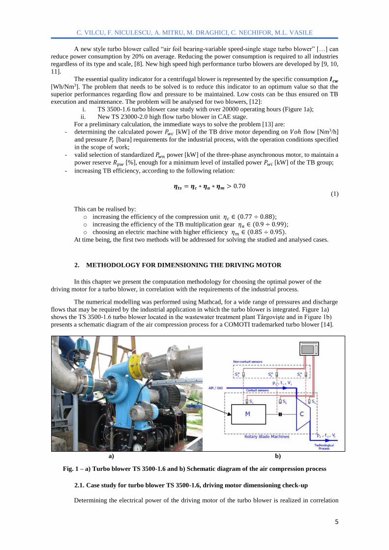
flows that may be required by the industrial application in which the turbo blower is integrated. Figure 1a)
shows the TS 3500-1.6 turbo blower located in the wastewater treatment plant Târgovişte and in Figure 1b)
presents a schematic diagram of the air compression process for a COMOTI trademarked turbo blower [14].
a) b)
Fig. 1 – a) Turbo blower TS 3500-1.6 and b) Schematic diagram of the air compression process
2.1. Case study for turbo blower TS 3500-1.6, driving motor dimensioning check-up
Determining the electrical power of the driving motor of the turbo blower is realized in correlation

Power correlation of driving motor for turbo blower with the industrial process
6
with the requirements of the process for which the TB is used for, specified in the scope of work for the given
application type. Thus, for the following operation domain imposed to TS 3500-1.6 turbo blower:
𝓛(𝑽𝒐𝒉, 𝝅𝒄) ≡ (3500, 1.6) [Nm3/h, #] (2)
the air weight flow Gas at the turbo blower inlet, depending on the inlet air temperature Tas, and the location
altitude Hs, is given by the relation:
𝑮𝒂𝒔(𝑻𝒂𝒔, 𝑯𝒔) = 𝑽𝒐𝒔 ∗ 𝝆𝒉(𝑻𝒂𝒔, 𝑯𝒔) = 𝑽𝒐𝒔 ∗𝑷𝒐
𝑹𝒂∗𝑻𝒂𝒔∗ 𝒆−
𝑴∗𝒈∗𝑯𝒔
𝑹∗𝑻𝒂𝒔 [kg/s] (3)
where the air volume flow per second (Vos) is given by the imposed hourly volume flow (Voh):
𝑽𝒐𝒔 =𝑽𝒐𝒉
𝟑𝟔𝟎𝟎= 0.972 [Nm3/s] (4)
and the air density ρh in the given location depends on the temperature variation in the ambient environment
Tas and on the atmospheric pressure at the altitude Hs in the location where the TB is installed.
For the following values of the constants: Po = 101325 [Pa]; To = 273.15 [°K]; Ra = 287.19 [J/kg*K];
M = 0.029 [kg/mol]; g = 9.81 [m/s2]; R = 8.31 [J/mol*K] and the variation domains of variables: 𝑇𝑎𝑠 =243.15 ÷ 323.15 [°K] and 𝐻𝑠 = 0, 100 ÷ 3000 [m], the variation of the air weight flow function Gas at TB
inlet, given by equation (3), is represented graphically in 3D coordinates in Figure 2a). For operation location
altitude (Hs = 260 m), the variation of Gas(Tas, Hs) function of temperature is represented graphically in 2D
coordinates in Figure 2b).
Considering the numerous factors which lead to increasing the operation temperature (high ambient
temperatures during summer, direct sunlight, heat generating equipment in proximity, etc.), it is recommended
that a heavy duty rate of the turbo blower to be chosen for a continuous operation (S1) of the driving motor.
This is due to the high temperatures on the inlet. For an average value Gam in Figure 2b) considered for inlet
air weight flow, correlated with the operation conditions in situ, we have:
𝑮𝒂𝒎 = 𝑮𝒂𝒔(303.15, 206) = 1.099 [kg/s] (5)
a) b)
Fig. 2 – a) Variation of air weight flow at TB inlet function of temperature (Ox) and altitude (Oy); b)
Variation of air weight flow at inlet function of temperature, for TS 3500-1.6
For TS 3500-1.6, we calculate the efficiency of the TB compression group, with relation (1), to be:
𝜼𝒕𝒔 = 0.83 ∗ 0.98 ∗ 0.92 = 0.748 (6)
For a polytropic state transformation of compressed air (k=1.4), the driving motor power for the turbo
blower is calculated with the relation:
𝑷𝒄𝒘 = 𝑮𝒂𝒎 ∗ (𝒌
𝒌−𝟏∗ 𝑹𝒂 ∗ 𝑻𝒂𝒎 ∗ (𝝅𝒄
𝒌−𝟏
𝒌 − 𝟏)) ∗𝟏𝟎−𝟑
𝜼𝒕𝒔= 66.666 [kW] (7)

C. VILCU, F. NICULESCU, A. MITRU, M. DRAGHICI, C. NECHIFOR, M.L. VASILE
7
The numerical modelling program NMPTB for the dimensioning of the driving motor enables the
graphic visualisation of the compressor shaft power Pc, as well as the minimum power Pw necessary for the
driving motor, considering the given application. The variation of these powers in [kW] with the suction air
temperature Tas is represented in Figure 3.
Fig. 3 – Variation with temperature Ta of driving motor power of TS 3500-1.6
(Pc [kW] – power at compressor shaft; Pw [kW] – motor power)
The standardized domain regarding manufacturing electrical power [kW] of three-phase asynchronous
motors, in which Pcw is inserted for comparison regarding choosing the driving motor for TB is presented in
the vector with the values of nominal powers Pwn below:
𝑷𝒘𝒏 = [75; 90; 110; 132; 160; 200; 250; 315; 355; 400; 450; 500; 550; 630; 710; 800; 1000] (8)
From the vector above, it is chosen the electrical power from the immediately superior class to the
calculated value Pcw. The difference between Pwn and Pcw will be the power reserve for the electrical machine
operation. For an optimal selection of the motor, the power reserve δP is recommended to be within the interval
of (5÷15)% from the nominal power Pwn. According to the value resulted in the previous programming
sequence for Pcw, we calculate with the presented algorithm:
𝒏 = 𝟓 ⊳ 𝑷𝒘𝒏𝟎,𝒏 = 75 [kW]; 𝜹𝑷 = 𝑷𝒘𝒏𝟎,𝒏 − 𝑷𝒄𝒘 = 8.334 [kW] (9)
Consequently, the following values result:
𝑹𝒑𝒘 = 𝟏𝟎𝟎 ∗𝜹𝑷
𝑷𝒘𝒏𝟎,𝒏= 11.11 [%] (10)
𝑾𝒎𝒔 = 𝟏𝟎𝟎 ∗𝑷𝒄𝒘
𝑷𝒘𝒏𝟎,𝒏= 88.89 [%] (11)
𝑰𝒄𝒘 = 𝟏𝟎𝟎𝟎 ∗𝑷𝒄𝒘
𝑽𝒐𝒉= 19.047 [Wh/Nm3] (12)
Based on the results obtained, it can be stated that the turbo blower TS 3500-1.6 has been properly
dimensioned with regard to the driving motor, due to the following reasons:
- By choosing a motor with nominal power 𝑃𝑤𝑛0,𝑛 = 75 [kW], the efficiency of the turbo blower group
is of 𝜂𝑡𝑠 = 0.748 and the compression ratio is of 𝜋𝑐 = 1.6, thus ensuring the necessary discharge air
flow of 𝑉𝑜ℎ = 3500 [Nm3/h] for wastewater biological (aeration) treatment;
- Loading the motor at only 𝑊𝑚𝑠 = 88.89 % of the nominal power enables the turbo blower to be used
successfully in heavy-duty operation conditions or to be used for a wide range of the technological
processes in the application category it was designed for;
- The quality indicator (technical and economical) 𝐼𝑐𝑤 = 19.047 [Wh/Nm3] of TS 3500-1.6, compared
with the one of same class turbo blowers but of different trademark, indicates an optimal selection
(quality/price) of the driving motor for our turbo blower.

Power correlation of driving motor for turbo blower with the industrial process
8
2.2. Driving motor dimensioning for high flow turbo blower TS 23000-2.0
It is proceeded directly to step #3 of NMPTB program. The calculated power of the driving
motor for the turbo blower, given by relation (7), is written as a function of three variables Pcw(πc,
Vos, Ta):
𝑷𝒄𝒘(𝝅𝒄, 𝑽𝒐𝒔, 𝑻𝒂) = 𝑽𝒐𝒔 ∗ 𝝆𝒂𝒎 ∗ (𝒌
𝒌−𝟏∗ 𝑹𝒂 ∗ 𝑻𝒂 ∗ (𝝅𝒄
𝒌−𝟏
𝒌 − 𝟏)) ∗𝟏𝟎−𝟑
𝜼𝒕𝒔 [kW] (13)
where we have:
- TB compression ratio vector: 𝜋𝑐 = 1.100 ÷ 2.500 [#]
- TB hourly discharge flow vector: 𝑉𝑜ℎ = 1000 ÷ 25000 [Nm3/h]
- Inlet air temperature vector: 𝑇𝑎 = 243.15 ÷ 323.15 [°K]
and parameter values: {𝑘, 𝑅𝑎, 𝜌𝑎𝑚, 𝜂𝑡𝑠} = {1.4; 287.19; 1.164; 0.748}
were established in the previous step of NMPTB program, according to the process.
For an imposed hourly volume flow of TB: 𝑉𝑜ℎ = 23 000 [Nm3/h], the function Pcw(πc,Vos,Ta)
given by relation (13) becomes:
𝑷𝒎𝒗(𝝅𝒄, 𝑻𝒂) =𝑽𝒐𝒉∗𝝆𝒂𝒎
𝟑𝟔𝟎𝟎∗ (
𝒌
𝒌−𝟏∗ 𝑹𝒂 ∗ 𝑻𝒂 ∗ (𝝅𝒄
𝒌−𝟏
𝒌 − 𝟏)) ∗𝟏𝟎−𝟑
𝜼𝒕𝒔 [kW] (14)
The variation graph in 3D coordinates of motor power 𝑃𝑚𝑣(𝜋𝑐, 𝑇𝑎) [kW] function of variables 𝜋𝑐
(Ox) and 𝑇𝑎 (Oy) is presented in Figure 4a). The curved mesh nodes from the spatial surface domain represent
the values for calculated power of the driving motor, necessary for obtaining the state vectors (p,V,T) of the
industrial process. For TS 23000 turbo blower model [Nm3/h], presently in CAE stage, the values of calculated
power are analysed for three representative nodes from the illustrate domain. These ones correspond to the
values of compression ratio 𝜋𝑐 ∈ {1.5; 2.0; 2.5} and are represented in Figure 4b).
a) b)
Fig. 4 – a) 3D variation graph for the power [kW] of driving motor for TS 23000 and
b) Variation of motor power Pmv [kW] with temperature Ta at constant πc
According to the values calculated for driving motor power in (14), the following nominal powers
Pwn will result, corresponding to the imposed compression ratio:
𝑃𝑚𝑣(1.5, 303.15) = 371.879 [kW] ⇒ 𝑃𝑤𝑛0,14 = 400 [kW] (15)
𝑃𝑚𝑣(2.0, 303.15) = 663.116 [kW] ⇒ 𝑃𝑤𝑛0,19 = 710 [kW] (16)
𝑃𝑚𝑣(2.5, 303.15) = 906.09 [kW] ⇒ 𝑃𝑤𝑛0,21 = 1000 [kW] (17)
In the graphs showing the variation of 𝑃𝑚𝑣 with TB inlet air temperature for the three compression
ratios 𝜋𝑐 analysed, the power reserves ensured by nominal powers can be easily identified through markers.
C. VILCU, F. NICULESCU, A. MITRU, M. DRAGHICI, C. NECHIFOR, M.L. VASILE
9
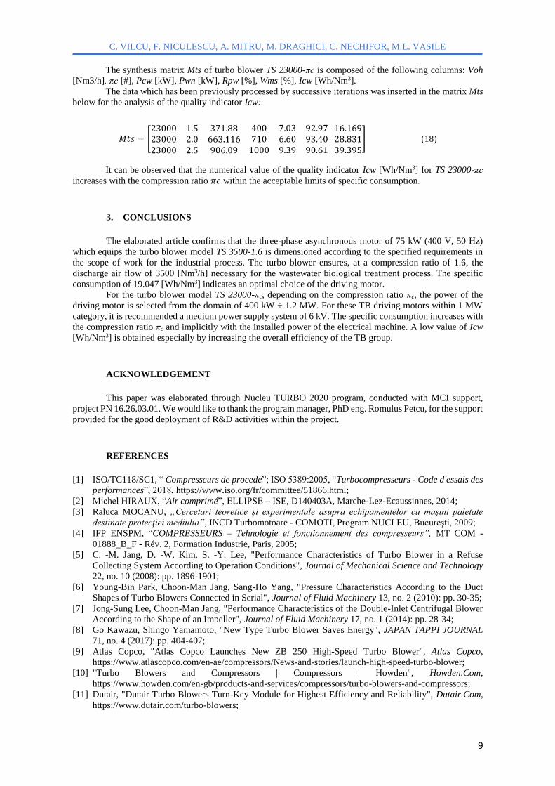
The synthesis matrix Mts of turbo blower TS 23000-πc is composed of the following columns: Voh
[Nm3/h], πc [#], Pcw [kW], Pwn [kW], Rpw [%], Wms [%], Icw [Wh/Nm3].
The data which has been previously processed by successive iterations was inserted in the matrix Mts
below for the analysis of the quality indicator Icw:
𝑀𝑡𝑠 = [23000 1.5 371.8823000 2.0 663.11623000 2.5 906.09
400 7.03 92.97710 6.60 93.40
1000 9.39 90.61
16.16928.83139.395
] (18)
It can be observed that the numerical value of the quality indicator Icw [Wh/Nm3] for TS 23000-πc
increases with the compression ratio 𝜋𝑐 within the acceptable limits of specific consumption.
3. CONCLUSIONS
The elaborated article confirms that the three-phase asynchronous motor of 75 kW (400 V, 50 Hz)
which equips the turbo blower model TS 3500-1.6 is dimensioned according to the specified requirements in
the scope of work for the industrial process. The turbo blower ensures, at a compression ratio of 1.6, the
discharge air flow of 3500 [Nm3/h] necessary for the wastewater biological treatment process. The specific
consumption of 19.047 [Wh/Nm3] indicates an optimal choice of the driving motor.
For the turbo blower model TS 23000-πc, depending on the compression ratio πc, the power of the
driving motor is selected from the domain of 400 kW ÷ 1.2 MW. For these TB driving motors within 1 MW
category, it is recommended a medium power supply system of 6 kV. The specific consumption increases with
the compression ratio πc and implicitly with the installed power of the electrical machine. A low value of Icw
[Wh/Nm3] is obtained especially by increasing the overall efficiency of the TB group.
ACKNOWLEDGEMENT
This paper was elaborated through Nucleu TURBO 2020 program, conducted with MCI support,
project PN 16.26.03.01. We would like to thank the program manager, PhD eng. Romulus Petcu, for the support
provided for the good deployment of R&D activities within the project.
REFERENCES
[1] ISO/TC118/SC1, “ Compresseurs de procede”; ISO 5389:2005, “Turbocompresseurs - Code d'essais des
performances”, 2018, https://www.iso.org/fr/committee/51866.html;
[2] Michel HIRAUX, “Air comprimé”, ELLIPSE – ISE, D140403A, Marche-Lez-Ecaussinnes, 2014;
[3] Raluca MOCANU, „Cercetari teoretice şi experimentale asupra echipamentelor cu maşini paletate
destinate protecţiei mediului”, INCD Turbomotoare - COMOTI, Program NUCLEU, Bucureşti, 2009;
[4] IFP ENSPM, “COMPRESSEURS – Tehnologie et fonctionnement des compresseurs”, MT COM -
01888_B_F - Rév. 2, Formation Industrie, Paris, 2005;
[5] C. -M. Jang, D. -W. Kim, S. -Y. Lee, "Performance Characteristics of Turbo Blower in a Refuse
Collecting System According to Operation Conditions", Journal of Mechanical Science and Technology
22, no. 10 (2008): pp. 1896-1901;
[6] Young-Bin Park, Choon-Man Jang, Sang-Ho Yang, "Pressure Characteristics According to the Duct
Shapes of Turbo Blowers Connected in Serial", Journal of Fluid Machinery 13, no. 2 (2010): pp. 30-35;
[7] Jong-Sung Lee, Choon-Man Jang, "Performance Characteristics of the Double-Inlet Centrifugal Blower
According to the Shape of an Impeller", Journal of Fluid Machinery 17, no. 1 (2014): pp. 28-34;
[8] Go Kawazu, Shingo Yamamoto, "New Type Turbo Blower Saves Energy", JAPAN TAPPI JOURNAL
71, no. 4 (2017): pp. 404-407;
[9] Atlas Copco, "Atlas Copco Launches New ZB 250 High-Speed Turbo Blower", Atlas Copco,
https://www.atlascopco.com/en-ae/compressors/News-and-stories/launch-high-speed-turbo-blower;
[10] "Turbo Blowers and Compressors | Compressors | Howden", Howden.Com,
https://www.howden.com/en-gb/products-and-services/compressors/turbo-blowers-and-compressors;
[11] Dutair, "Dutair Turbo Blowers Turn-Key Module for Highest Efficiency and Reliability", Dutair.Com,
https://www.dutair.com/turbo-blowers;

Power correlation of driving motor for turbo blower with the industrial process
10
[12] "COMOTI - Romanian Research and Development Institute for Gas Turbines", Comoti.Ro,
http://www.comoti.ro/en/Suflante-centrifugale-de-aer.htm;
[13] Essi Paavilainen, “The performance and the characteristic field of a centrifugal compressor”, Lappeenranta
University of Technology, BH10A0200, Lappeenranta, 2008;
[14] Constantin VÎLCU, „Cercetări privind automatizarea maşinilor paletate de înaltă turaţie”, INCD
Turbomotoare - COMOTI, Program NUCLEU, Bucureşti, 2009
TURBO, vol. V (2018), no. 2
11
ADJUSTING THE RESONANT FREQUENCY OF A
CANTILEVER PIEZOELECTRIC HARVESTER
Claudia BORZEA1, Daniel COMEAGĂ2
ABSTRACT: The paper presents the methods employed for adjusting the resonant frequency of a piezoelectric
harvester in cantilever construction, in order to meet the resonance condition with the vibration source.
Operating at resonance is the foremost requirement for obtaining maximum electrical response. A sharp voltage
peak occurs at that frequency, significant electric power being obtained in a tight frequency range. The
frequency can be changed in various ways, such as: modifying the length subjected to vibrations by changing
clamp position, using a more elastic or stiffer fastening, adding a proof mass, electric loads, etc. The aim of
this work is to modify the fundamental frequency of the piezoelectric transducer so as to match the frequency
of the test vibrating engine measured at ~190 Hz. A FEM simulation has been realized in COMSOL
Multiphysics, to have an idea beforehand of what we can expect. The experimental tests have shown a close
similitude with the simulation results, thus validating the finite element method model. The desired frequency
was eventually obtained, the structure resonating with source vibrations.
KEYWORDS: Energy Harnessing, Piezoelectric Harvester, Vibrations, Frequency, FEM Analysis
NOMENCLATURE
CAD – Computer Aided Design;
FEM – Finite Element Method;
FR4 – Flame Retardant Type 4 (woven glass reinforced epoxy resin);
PZT – Lead Zirconate Titanate;
rpm – Revolutions per minute;
f [Hz] – Frequency;
g [m/s2] – Gravitational acceleration;
* The other symbols and notations used are explained throughout the paper.
1. INTRODUCTION
Piezoelectric materials exhibit the property that, when subjected to mechanical strain, they produce electric
charge proportional with the stress applied. Piezoelectric harvesters use the piezoelectric effect for the direct
conversion of mechanical vibrations into electrical energy, and tap this energy by connecting the harvester
electrodes with an electric circuit [1]. In order to achieve maximum electrical response, it is preferable to excite
a given harvester at its fundamental resonance frequency (or at one of the higher resonance frequencies) [2].
Resonance is a phenomenon in which a dynamic force drives a structure to vibrate at its natural frequency.
When a structure is in resonance, a small force can produce a large vibration response [3]. Since the foremost
requirement for energy scavenging devices is to operate in resonance at the excitation frequency, several
methods have been studied for adjusting the resonant frequency, described in [4]. It is noteworthy to remark
that even a slight deviation (± 1 Hz) from the resonant condition will result in a sudden drop in generated power
[5] for lightly damped systems. Using a higher damping for widening the frequency response near resonance
also leads to a decrease of the response, so it is not an optimum solution. Some structural, mechanical and
electronic solutions are currently being studied with the purpose of harvesting vibrations on a wider frequency
band. However, these techniques often exhibit hysteretic responses or high power consumption, which may
lead in inefficient results [6].
1 Romanian Research and Development Institute for Gas Turbines COMOTI, Department of
Automation and Electrical Engineering. 2 University Politehnica of Bucharest, Faculty of Mechanical Engineering and Mechatronics,
Department of Mechatronics and Precision Mechanics.
C. BORZEA, D. COMEAGĂ
12
Piezoelectric energy harvesting from ambient vibration sources has great potential for powering
microelectronic devices and wireless sensors. Almost all the conventional piezoelectric energy harvesters in
the literature have been designed with a single metallic layer as substrate along with the piezoelectric material
bonded over it [7]. Unimorph and bimorph beams have been modelled using FEM in [8, 9, 10, 11].
The harvester proposed in this paper, Midé PPA-4011, is a more complex quadmorph multilayer
beam. It consists of 17 very thin layers, including four PZT-5H piezoelectric wafers, each of them sandwiched
between a pair of thin copper electrodes, and each of these four sandwiches being separated by protection FR4
layers. The layers are bonded together by epoxy resin films. The total thickness is 1.32 mm. Such a structure
is more complex and more difficult to analyse and simulate using FEM programs.
The article presents the methods employed for adjusting the fundamental frequency (first natural
frequency) of the piezoelectric transducer, without affecting the electric power generated. The aim is to match
as possible the frequency of the source generating the vibrations. A voltage peak occurs at resonance, and the
voltage response would theoretically be infinite if the harvester had zero damping whatsoever. Practically this
is impossible, as many factors contribute to damping and attenuating the signal, such as: cables and electrical
connections resistances, internal damping, friction between layers, friction with air, etc.
2. METHODS FOR CHANGING NATURAL FREQUENCY
The piezoelectric transducer has been chosen so as to operate in the frequency range of engines,
compressors and other equipment owned by COMOTI. A Klimov TV2-117A gas turbine turboshaft engine
was chosen for running tests on. Rotational speeds measured beforehand vary between 10,000 and 14,000 rpm
at an acceleration of 0.9g (8.829 m/s2) in the point where mounting the accelerometer was possible. Knowing
that 1 rpm =1
60Hz, the frequency range is between 166 ÷ 233 Hz. In the mounting location, the frequency of
vertical vibration component is 190 Hz (11,400 rpm) [12]. When choosing the mounting spot, it has to be also
taken into consideration that the harvester is not able to withstand very high temperatures.
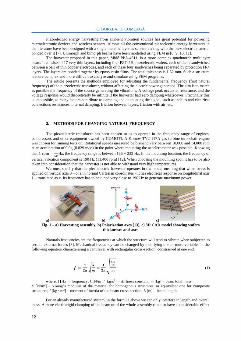
We must specify that the piezoelectric harvester operates in d31 mode, meaning that when stress is
applied on vertical axis 3 – or z in normal Cartesian coordinates – it has electrical response on longitudinal axis
1 – translated as x. Its frequency has to be tuned very close to 190 Hz to generate maximum power.
a) b) c)
Fig. 1 – a) Harvesting assembly, b) Polarization axes [13], c) 3D CAD model showing wafers
thicknesses and axes
Naturals frequencies are the frequencies at which the structure will tend to vibrate when subjected to
certain external forces [3]. Mechanical frequency can be changed by modifying one or more variables in the
following equation characterising a cantilever with rectangular cross-section, constrained at one end.
𝒇 =𝟏
𝟐𝝅√
𝒌
𝒎=
𝟏
𝟐𝝅√
𝟑𝑬𝑰
𝑳𝟑
𝒎 (1)
where: f [Hz] – frequency; k [N/m] / [kg/s2] – stiffness constant; m [kg] – beam total mass;
E [N/m2] – Young’s modulus of the material for homogenous structures, or equivalent one for composite
structures; I [kg ∙ m2] – moment of inertia of the beam cross-section; L [m] – beam length.
For an already manufactured system, in the formula above we can only interfere in length and overall
mass. A more elastic/rigid clamping of the beam or of the whole assembly can also have a considerable effect

Adjusting the resonant frequency of a cantilever piezoelectric harvester
13
upon natural frequency, modifying system stiffness. For composite structures, k is the equivalent stiffness, and
depends on layers’ elasticity modules, thicknesses and positions. A cantilever subjected to vibrations behaves
like a mass-spring-damper system. Hence, the first part of equation (1) is very similar, but the detailed
expression describes the cantilever more particularly. The number of natural frequencies or vibration modes
depends on the degrees of freedom of the system.
It is very important to mention that piezoelectric transducers are also affected by electrical loads,
which are able to change both frequency and electric response. The basic principle of electrical tuning is to
change the electrical load, the external impedance, which causes the power response spectrum of the generator
to shift. The resonant frequency as well as the output power reduce with increasing the damping part of the
electrical load [4].
3. FEM SIMULATION
In order to have an idea on system’s behaviour to be expected, a FEM model has been developed and
analysed in COMSOL Multiphysics, using the MEMS (Micro-Electro-Mechanical Systems) Module, for
analysing piezoelectric microscale behaviour. A multiphysics approach must be used, since connecting Solid
Mechanics with Electrostatics is essential for studying the piezoelectric effect. COMSOL Multiphysics is well
known for this possibility, and is preferred when it comes to the interconnection of multiple physics.
Fig. 2 – COMSOL Multiphysics interface and elaborated FEM model
Since the beam was declared attached to the clamp bars, considered perfectly stiff, the
eigenfrequencies were expected to be slightly higher than the real natural frequencies of the physical model.
The materials were declared accordingly, also modifying the default materials in COMSOL with the values
given in product specifications. An acceleration of 0.9g was applied to the base of the inferior clamp bar.
a) b) c) Fig. 3 – Clamping positions shown on 3D CAD model: a) rear clamp, b) middle clamp, c) front clamp
The simulation was performed for the clamping positions indicated in Fig. 3. The multilayer beam was designed
manually according to product specifications, and assembled with mounting kit parts downloaded from
manufacturer’s website [14]. Every parameter and input data was declared so as to match as possible the real
physical characteristics and conditions, in order to obtain a reliable FEM analysis.

C. BORZEA, D. COMEAGĂ
14
The simulation results are presented in Fig. 4. The most convenient clamping position is the rear clamp
because the frequency is minimum and slightly higher than the desired value. The frequency can be furthermore
decreased by adding a proof mass, but adding a heavier mass will result in higher stresses and thus a shorter
product lifetime. Rear clamping also enables a higher amplitude when vibrating (0.16 mm as against 0.12 mm
for middle clamp, at resonance). The piezoelectric response is proportional with the deformation. Therefore, in
this location more electrical power is generated.
a) 242.36 Hz (1st mode, 0.16 mm) b) 1089.7 Hz (2nd mode) c) 313.64 Hz (1st mode, 0.12 mm)
Fig. 4 – a) 1st bending mode and b) torsional mode for rear clamp, c) 1st resonance for middle clamp
From the beginning, it was desired to know the resonant frequency that would produce a torsional
mode, and avoid stimulating the harvester with vibrations at this frequency. No electrical charge is produced
at torsion (Fig. 4b) because one side bends upwards and the other side bends downwards, one side giving
positive charge and the other negative charge, which cancel each other, resulting in an overall net zero charge.
Torsional mode occurs around 1 kHz and it is safe, being too high to be reached in our application.
a) 242.36 Hz (3.47 V) b) 313.64 Hz (3.19 V)
Fig. 5 – Comparison between voltages computed for a) rear clamp and b) middle clamp
4. EXPERIMENTAL TESTS
The ideal clamping location was established within the simulation. Subsequently, several series of
experimental tests have been conducted. The experimental setup used consists of:
Signal analyser with integrated functions generator (Stanford SR785).
Shaker table (TIRA S 513) driven by and connected to the output of the signal analyser via amplifier.
Vibration meter with incorporated signal amplification (Brüel&Kjær type 2511, designed for high
impedance piezoelectric accelerometers). To this vibration meter, used as impedance adaptor and
amplifier, therefore as electric charge to voltage converter, the piezo generator was connected. The
output from the amplifier enters in channel 2 of the analyser.
Accelerometer (Brüel&Kjær type 4507-B-006), mounted on shaker and used as reference input signal.
This one is an ICP (Integrated Circuit Piezoelectric) accelerometer, with built-in preamplifier, and was
connected to input channel 1 of the analyser. ICP type power supply was activated for this channel.
The piezoelectric harvester was connected to the input of the vibration meter, which realizes the direct
conversion from electric charge to voltage. This is the optimum solution, yet very voluminous. The common
solution is to make the conversion with a resistor of very high values – not very efficient in practice but a
simple solution during experiments. The shaker table was driven with a swept-sine excitation signal generated
by the analyser, which displays frequency and voltage response of the piezoelectric transducer.

Adjusting the resonant frequency of a cantilever piezoelectric harvester
15
a) b) Fig. 6 – a) Experimental setup in Mechatronics department laboratory, b) Schematic diagram
Data was extracted at every 1 Hz and was saved from the signal analyser. First tests were conducted
with the assembly fastened in screws on the shaker table, and using a 5.5 kΩ resistor to measure voltage drop.
A resonant frequency was recorded at 205.25 Hz, as expected lower than computed in simulation due to a less
stiffness clamping and using an electrical resistance in tests. The voltage drop measured on the resistor was
428.7 mV/(m/s2), as shown in Fig. 7a). The graph in Fig. 7b) presents the transfer function for resistor voltage
drop vs. base acceleration, which was drawn with the data acquired from the analyser.
a) b) Fig. 7 – a) Frequency and voltage response read on the signal analyser [15], b) Voltage response graph
According to the equation below, the voltage that would be generated per gravitational acceleration
unit and at the 0.9g acceleration of the test engine is:
𝑈0,9𝑔 = 428,7 𝑚𝑉
(𝑚
𝑠2)∙ (0,9 ∙ 9,81
𝑚
𝑠2) ≅ 3,77 𝑉 (2)
After measuring the resistance of the wireless transmission integrated circuits board at ~2.5 kΩ, we
interconnected in series a 2.4 kΩ resistor. This one simulates best the electrical load of the circuit to be powered
by the harvester, since 2.5 kΩ resistors do not exist. For the second set of tests, we fixed the assembly with
elastic adhesive tape on the shaker table, making it less stiff. However, this is not a reliable solution for
attaching the assembly on the engine, and can only be used in tests. A thin elastic layer can be placed
underneath, with various elasticities and thicknesses, damping the assembly fixed in screws.
The resulted resonant frequency was 201.25 Hz, recording a 4 Hz decrease from the first tests with
screw mount. The voltage measured was 225 mV/(m/s2). At 0.9g acceleration we have:
𝑈0,9𝑔 = 225 𝑚𝑉
(𝑚
𝑠2)∙ 8,829
𝑚
𝑠2 ≅ 2 𝑉 (3)
0
50
100
150
200
250
300
350
400
450
500
150 160 170 180 190 200 210 220 230 240 250
Vo
ltag
e re
spo
nse
/acc
eler
atio
n
[mV
/(m
/s2)
]
Frequency [Hz]
Voltage response graph [mV/(m/s2)]
C. BORZEA, D. COMEAGĂ
16
It is observed that the solution with intermediary elastic layer leads to a change in resonant frequency,
but attenuates the electric response as well. Therefore, it can only be used as a quick solution for short-term
testing conditions.
Using a higher electric resistance increases the voltage drop. However, increasing the resistance is not
a solution to our application because the current drops, and this reduces power. Transmitting a wireless signal
requires 20 mW electrical power, at a rated current of 2 mA. Applying the relation = 𝑈 ∙ 𝐼 = 𝑅 ∙ 𝐼2 , the output
voltage required at 2 mA would be 5 V.
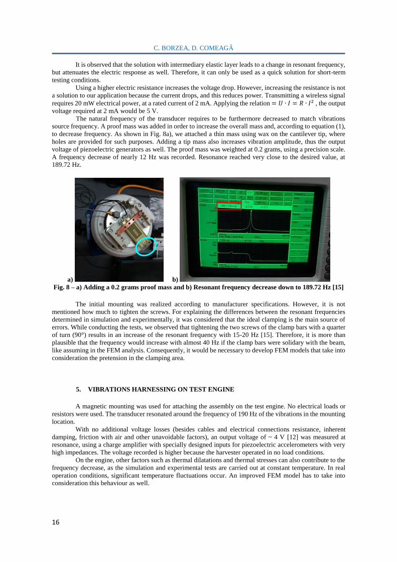
The natural frequency of the transducer requires to be furthermore decreased to match vibrations
source frequency. A proof mass was added in order to increase the overall mass and, according to equation (1),
to decrease frequency. As shown in Fig. 8a), we attached a thin mass using wax on the cantilever tip, where
holes are provided for such purposes. Adding a tip mass also increases vibration amplitude, thus the output
voltage of piezoelectric generators as well. The proof mass was weighted at 0.2 grams, using a precision scale.
A frequency decrease of nearly 12 Hz was recorded. Resonance reached very close to the desired value, at
189.72 Hz.
a) b) Fig. 8 – a) Adding a 0.2 grams proof mass and b) Resonant frequency decrease down to 189.72 Hz [15]
The initial mounting was realized according to manufacturer specifications. However, it is not
mentioned how much to tighten the screws. For explaining the differences between the resonant frequencies
determined in simulation and experimentally, it was considered that the ideal clamping is the main source of
errors. While conducting the tests, we observed that tightening the two screws of the clamp bars with a quarter
of turn (90°) results in an increase of the resonant frequency with 15-20 Hz [15]. Therefore, it is more than
plausible that the frequency would increase with almost 40 Hz if the clamp bars were solidary with the beam,
like assuming in the FEM analysis. Consequently, it would be necessary to develop FEM models that take into
consideration the pretension in the clamping area.
5. VIBRATIONS HARNESSING ON TEST ENGINE
A magnetic mounting was used for attaching the assembly on the test engine. No electrical loads or
resistors were used. The transducer resonated around the frequency of 190 Hz of the vibrations in the mounting
location.
With no additional voltage losses (besides cables and electrical connections resistance, inherent
damping, friction with air and other unavoidable factors), an output voltage of ~ 4 V [12] was measured at
resonance, using a charge amplifier with specially designed inputs for piezoelectric accelerometers with very
high impedances. The voltage recorded is higher because the harvester operated in no load conditions.
On the engine, other factors such as thermal dilatations and thermal stresses can also contribute to the
frequency decrease, as the simulation and experimental tests are carried out at constant temperature. In real
operation conditions, significant temperature fluctuations occur. An improved FEM model has to take into
consideration this behaviour as well.

Adjusting the resonant frequency of a cantilever piezoelectric harvester
17
Fig. 9 – Vibrations harnessing on a Klimov TV2-117A gas turbine turboshaft engine
6. CONCLUSIONS
Overall, the results are encouraging for harnessing the kinetic energy from vibrating machinery for
the energy supply of low-power wireless sensors. By harnessing inherent vibrations, it is possible to eliminate
the need for batteries and electrical cables. Theoretically, such an energy harvesting source can function for an
unlimited period of time, rendering the wireless sensors autonomous.
In order to obtain maximum electrical response, a piezoelectric transducer has to operate at resonance
with the vibration source. Thus, the virtual length of the cantilever, the overall mass and the stiffness of the
tested assembly have been adjusted in order to set the fundamental frequency of the harvester as close as
possible to the test engine frequency.
A preliminary FEM model was analysed to evaluate the expected results regarding performance,
frequency range and von Mises stresses. Several techniques have been practically employed for tuning the
frequency: using different mounting methods (screw mount, double-adhesive tape, magnetic mount, as well as
perfectly stiff mount in simulation); changing the clamping position for enabling the most convenient virtual
length to vibrate; adding a proof mass; using different electric loads and resistances. At the same time, the
electrical response was monitored with adequate equipment, measuring the output power generated.
The electric energy from a single harvester is not sufficient for powering the circuit board. Thus,
further research will focus on mounting all the three available harvesters on the same support and connecting
them electrically in series. There is a high risk that two of them to vibrate in antiphase, in which case one of
the electric charges generated will be positive and the other negative, thus nullifying each other if connected in
the same electric circuit. To avoid such inconvenient situations, Schottky diodes will be used for the
rectification of the alternate current yielded by piezoelectric transducers, and converting it into direct current
cumulated from all the three devices. Schottky diodes are known for their low forward voltage, making them
ideal for our application, since a significant voltage drop on the diodes is undesirable. Ensuring a capacitor or
accumulator in the circuit is also taken into consideration for storing energy and delivering it when necessary.
ACKNOWLEDGEMENT
We would like to thank INCDT COMOTI for the resources provided, with special thanks to eng.
Adrian Stoicescu, PhD eng. Sorin Gabroveanu, and PhD eng. Romulus Petcu for advice and for acquiring the
devices within “Nucleu” Program TURBO 2020, project number PN 16.26.07.01.
REFERENCES
[1] A.M. Matos, J.M. Guedes, K.P. Jayachandran and H.C. Rodrigues, "Computational Model for Power
Optimization of Piezoelectric Vibration Energy Harvesters with Material Homogenization", in Computers
& Structures 192 (Elsevier, 2017): pp. 144-156;

C. BORZEA, D. COMEAGĂ
18
[2] A. Erturk and D. J. Inman, "An Experimentally Validated Bimorph Cantilever Model for Piezoelectric
Energy Harvesting from Base Excitations", in Smart Materials and Structures 18, no. 2 (IOP Publishing,
2009): 025009 (18pp);
[3] "Natural Frequency and Resonance", Siemens PLM Community, accessed 22.11.2018,
https://community.plm.automation.siemens.com/t5/Testing-Knowledge-Base/Natural-Frequency-and-
Resonance/ta-p/498422;
[4] Dibin Zhu, Michael J. Tudor and Stephen P. Beeby, “Strategies for Increasing the Operating Frequency
Range of Vibration Energy Harvesters: A Review”, in Measurement Science and Technology, Vol. 21,
no. 2 (IOP Publishing, 2010): 022001 (29pp);
[5] Roberto Montanini and Antonino Quattrocchi, "Experimental Characterization of Cantilever-Type
Piezoelectric Generator Operating at Resonance for Vibration Energy Harvesting", in Proceedings of the
12Th International A.I.VE.LA. Conference on Vibration Measurements by Laser and Noncontact
Techniques, AIP Conference Proceedings 1740, 060003 (2016);
[6] Adrien Morel, Romain Grézaud, Gaël Pillonnet and Adrien Badel, "Piezoelectric Generator Frequency
Tuning and Output Power Optimization through the Use of an Electronic Interface", in 11Th Energy
Harvesting Workshop, 2016;
[7] Xiangyang Li, Deepesh Upadrashta, Kaiping Yu and Yaowen Yang, "Sandwich Piezoelectric Energy
Harvester: Analytical Modeling and Experimental Validation", in Energy Conversion and Management
176 (2018): pp. 69-85;
[8] Tithi Desai, Ravishankar Dudhe and Sumathi Ayyalusamy, "Design, Simulation and Optimization of
Bimorph Piezoelectric Energy Harvester Using COMSOL Multiphysics", in Proceedings of the 2016
COMSOL Conference, Bangalore, 2016, pp. 1-4;
[9] N. F. Rahim, N. R. Ong, M. H. A. Aziz, J. B. Alcain, W. M. W. N. Haimi, and Z. Sauli, "Modelling of
Cantilever Based on Piezoelectric Energy Harvester", in 3rd Electronic and Green Materials
International Conference 2017 (EGM 2017), AIP Conference Proceedings 1885, 020301 (2017);
[10] M. N. Uddin, M. S. Islam, J. Sampe, S. H. M. Ali and M. S. Bhuyan, "Design and Simulation of
Piezoelectric Cantilever Beam Based on Mechanical Vibration for Energy Harvesting Application", in
2016 International Conference on Innovations in Science, Engineering and Technology (ICISET), Dhaka,
2016, pp. 1-4;
[11] Giuseppe Acciani, Filomena Di Modugno and Giancarlo Gelao, "Comparative Studies of Piezoelectric
Harvester Devices", in Energy Harvesting, Technology Methods and Applications, Renee Williams and
Ali Bakhshandeh Rostamied. (Nova science Publishers, 2016), pp. 1-18;
[12] Adrian Stoicescu, Claudia Borzea, Romeo Hrițcu, Marius Deaconu, Cristian Nechifor, Daniel Olaru,
„Cercetări privind realizarea de sisteme de comandă și control pentru turbomotoare și turbomașini în
general, ce să răspundă noilor cerințe ale beneficiarilor” (“Researches Regarding the Realization of
Command and Control Systems, to Respond to Beneficiaries’ New Requirements”, Nucleu Program,
Phase 8, PN 16.26.07.01-8 (Bucharest, 2017);
[13] „Piezoelectric Constants | Elastic Compliance | APCI”, Americanpiezo.Com, accessed 27.10.2018,
https://www.americanpiezo.com/knowledge-center/piezo-theory/piezoelectric-constants.html;
[14] Mide Technology, accessed 28.10.2018, https://www.mide.com/collections/piezo-protection-advantage-
ppa;
[15] Claudia Irina Borzea, „Sistem de monitorizare pentru instalațiile de comprimare gaz metan, cu recuperare
de energie” (“Monitoring System for Methane Gas Compression Installations, with Energy Harnessing”),
Master’s Thesis, Master of Advanced Mechatronics, Faculty of Mechanical Engineering and
Mechatronics, University Politehnica of Bucharest, 2018.

TURBO, vol. V (2018), no. 2
19
OIL-FREE SCREW COMPRESSOR FLOW
EVALUATION
Mihnea GALL1, Vlad Alexandru POPA1, Ion MĂLĂEL1
ABSTRACT:Numerical simulations are useful tools to predict the change in overall performance when
optimization criteria are applied to screw compressors. The aim of this paper is to present the methodology of
setting up an unsteady computational fluid dynamics (CFD) simulation for an oil-free screw compressor
followed by a post-processing of results. The TwinMesh commercial software was used for meshing purpose
for rotors domains, whereas the simulation and the post-processing of results were performed in Ansys CFX.
The turbulence models used in this flow modeling are standard k-ε and standard k-ω coupled by the Sheer
Stress Transport (SST) model. The results consist of the total power variation, the torque variation, the
meridional variation of absolute pressure from inlet to outlet and last but not least the mass flow variation. This
kind of work is going to be extremely valuable for future numerical studies on the performance of screw
compressors.
KEYWORDS: screw compressor, CFD, oil-free, volumetric efficiency.
NOMENCLATURE
𝐸- total energy
𝐻- total enthalpy
Pr - Prandtl number
R - air constant
T - temperature
𝑐𝑝- specific heat
𝑒- specific internal energy
ℎ- specific enthalpy
λ – thermal conductivity
𝑚- mass
𝑝- instantaneous static pressure
�̅� - mean static pressure
𝒒𝒊 - heat-flux vector
𝒕 - time
𝒖𝒊 - instantaneous velocity in tensor notation
𝒖�̃�- Favre averaged velocity
𝒖𝒊′′̃- Favre fluctuating velocity in tensor notation
𝒙𝒊- position vector in tensor notation
𝜹𝒊𝒋- Kronecker delta
𝝉𝒊𝒋 - viscous stress tensor
𝝆 - mass density
𝝁 - dynamic molecular viscosity
𝝂 - kinematic molecular viscosity
1. INTRODUCTION
A screw compressor is a type of compressor that uses a rotary-type positive-displacement mechanism
with two helical rotors, a male rotor and a female rotor. The rotors consist of a number of a lobes that can differ
between the male and the female. The male rotor is being electrically set and in turn operates the female rotor.
The helical surfaces and the housing around the compressor rotors enclose the cavity volume of the compressor.
In this paper, an oil-free screw compressor is studied. In this kind of compressor configuration, the
working chamber operates free of oil, thus eliminating the efficiency losses due to shear stresses.
Optimizing screw compressors is of high interest nowadays as the operating principle of such
machines is identical to that developed in the late 19th century [1]. As the electricity consumption represents
approximately 80% of the total lifecycle cost of the screw compressor [2], even a slight decrease in overall
power consumption of the machine will lead to important savings.
There are a lot promising optimization criterion related to the development of both male and female
1Romanian Research and Development Institute for Gas Turbines COMOTI, Bucharest, Romania

M. GALL, V.A. POPA, I. MALAEL
20
of both male and female profiles, casings and reduced gaps, but all of these ideas have to be evaluated somehow
and validated too.
Performance studying of screw compressors can be made both analytical and numerical [3], but
Kennedy et al. conclude that pressure ratio has a great influence on the results, while operating at increased
speeds reduces the difference between the two models. Thus, as Raneet al. also stated [6] a better insight into
the evaluation of screw compressor performance is obtained by using CFD rather than using analytic chamber
models.
The CFD methods for the oil-free screw compressor performance assessment leads to unsteady flow
simulations with moving boundaries. The screw compressor operation involves a continuous variation of the
volume between the male, the female and the casing. The numerical simulation of such configurations brings
some difficulties in terms of meshing strategies [7].There are a lot of studies regarding different techniques and
methodologies. [3][4] However, this issue remains the main challenge of such a simulation, as there is no
commercial standard computing grid able to do deforming mesh [7]. The sliding interface between the male
and the female subdomains represent a complex challenge in terms of meshing [9]. Often, coarse mesh along
the interface is obtained which leads to numerical errors during computation. Fortunately, specialized reliable
software, TwinMesh, was developed in the last few years in order to compute mesh for a screw compressor
simulation [5]. In their CFD simulation of screw compressor, Ding and Jiang [8] employed SCORG and
Simerics, another dedicated software for positive displacement machines, to generate the mesh files for
different rotation angles of the rotor.
An analytical approach into computing the performance of a screw compressor can yield results in
several seconds in contrast to a numerical simulation which is both very time and memory consuming.
However, a CFD simulation is able to provide an extensive range of results which can be post-processed. This
way, a numerical simulation presents some advantages from the point of view of a researcher which can observe
the flow phenomena and the change in overall performance by implementing some optimization measurements.
An accurate flow prediction, heat transfer, interaction between the fluid and the walls was obtained by means
of CFD analysis by Kovacevic et al. [10] [11]
Consequently, it is very important to develop a methodology of setting up a numerical simulation for
assessing the oil-free screw compressor performance. This is going to be valuable for both future fundamental
and experimental research.
2. THEORETICAL APPROACH
The best currently available approach to determine the instantaneous fields of great interest in an oil-
free screw compressor (pressure, velocity, temperature) and the overall performance of the machine too is
represented by the numerical integration of the fluid flow equations. However, the numerical algorithms have
to be validated previously, either by comparing the results on simple geometries with experimental or analytical
data, or by comparing the results with those yielded by other algorithms already validated.Fluid flows are
described by the Navier-Stokes equations system. One of the most commonly used mathematical models for
numerical simulation of turbulence is the Reynolds averaged equations, known in the literature as RANS -
Reynolds Averaged Navier Stokes or URANS for unsteady flows. For unsteady compressible flows, the
URANS system expressed in tensor notation with Einstein convention can be written as follows:
• the transport equation for mass:
( )0
~=
+
i
i
x
u
t
(1)
• the transport equation for momentum:
( ) ( )
−
+
−=
+
,,,,~~~
jiijji
jij
i uuxx
puu
xt
u
(2)
• the transport equation for energy:
( ) ( )j ij i ij i ij jij j j
TE u H u u u u H
t x x x
+ = + + − +
(3)

Oil-free screw compressor flow evaluation
21
An additional equation to the system (1)-(3) is represented by the state equation:
RTp = (4)
An analytical approach to solve this system is rather impossible, thus a numerical integration in time
and space using CFD commercial software can solve the problem. However, the numerical schemes and
methods have to be carefully chosen because this kind of approach can yield an inaccurate solution due to
numerical errors and truncation caused by the approximation of partial derivatives with finite differences. For
temporal and spatial accuracy of such numerical simulation, the time and length scales of integration have to
be at least of the same order with the scales of the physical phenomenon.
3. NUMERICAL SIMULATION
3.1. Machine configuration
This paper evaluates numerically the performance of an oil-free screw compressor with a
configuration of 5 male lobes and 7 female lobes (Fig.1). The male rotor has an outer diameter of 83,2 mm,
whereas the female rotor outer diameter is 76,8 mm. Both rotors have a shaft of 35 mm. As the axial length of
both the rotors is 133,12 mm, the L/D ratio for male is 1.6 and 1.733 for female respectively. The distance
between the two rotating axis is 64 mm. The male pitch angle is 72⁰, while the wrap angle of rotors is 300⁰.
Fig. 1 Oil free screw compressor configuration Fig. 2 Stator parts
3.2. Domain details
The computational domain has both moving parts (male and female rotors) and static parts (suction
port and discharge port). Starting from the 3D CAD model of the oil-free screw compressor, the parts belonging
to stator were defined by using substraction and union functions of Ansys Design Modeler software (Fig. 2).
As stated before, the rotor meshing represents the major problem in such a numerical simulation.
TwinMesh commercial software was used not only to define the geometry of the rotors, but also to compute
their mesh for future simulations. By employing the TwinMesh commercial software, the rotors’ profiles are
imported as data points from Solidworks.
After defining the boundaries of both the rotor and the stator, the casing and the interface had to be
associated to curves. The interface between the male and the female rotor is automatically generated and needs
an overlapping assessment.
M. GALL, V.A. POPA, I. MALAEL
22
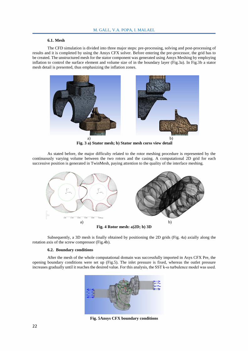
6.1. Mesh
The CFD simulation is divided into three major steps: pre-processing, solving and post-processing of
results and it is completed by using the Ansys CFX solver. Before entering the pre-processor, the grid has to
be created. The unstructured mesh for the stator component was generated using Ansys Meshing by employing
inflation to control the surface element and volume size of in the boundary layer (Fig.3a). In Fig.3b a stator
mesh detail is presented, thus emphasizing the inflation zones.
a) b)
Fig. 3 a) Stator mesh; b) Stator mesh corss view detail
As stated before, the major difficulty related to the rotor meshing procedure is represented by the
continuously varying volume between the two rotors and the casing. A computational 2D grid for each
successive position is generated in TwinMesh, paying attention to the quality of the interface meshing.
a) b)
Fig. 4 Rotor mesh: a)2D; b) 3D
Subsequently, a 3D mesh is finally obtained by positioning the 2D grids (Fig. 4a) axially along the
rotation axis of the screw compressor (Fig.4b).
6.2. Boundary conditions
After the mesh of the whole computational domain was successfully imported in Asys CFX Pre, the
opening boundary conditions were set up (Fig.5). The inlet pressure is fixed, whereas the outlet pressure
increases gradually until it reaches the desired value. For this analysis, the SST k-ω turbulence model was used.
Fig. 5Ansys CFX boundary conditions

Oil-free screw compressor flow evaluation
23
7. RESULTS AND DISCUSSIONS
Ansys CFX Post was used for post-processing purposes. Fig.6a presents the variation of total pressure
along the compressor. Starting from the inlet port (blue colour on top), the pressure increases from 1 bar to 4
bar at the discharge port (red colour on bottom). Fig.6b shows a 3D view of the rotors along with the inlet and
the discharge ports. Fig. 6c offers a more detailed view on the compression which takes place between the
rotors.
a) b)
c)
Fig. 6 Total pressure: a) Cross section; b) 3D view; c) Contours on rotors’walls
Using the pressure-pressure boundary conditions, both the inlet and the outlet, mass flow variation
were computed in Fig.7 for a whole rotation of the compressor. Whereas the inlet mass flow slightly oscillates
around 0.05 kg/s, the outlet mass flow presents a sharp variation. A maximum value of 0.17 kg/s is recorded
on outlet around 72⁰, 216⁰ and 340⁰. In contrast, the pulsating operating condition of the compressor is
emphasized by the positive values of the outlet mass flow in the following ranges 0⁰-50⁰, 110⁰-170⁰, 250⁰-300⁰.
M. GALL, V.A. POPA, I. MALAEL
24
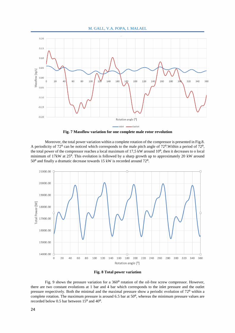
Fig. 7 Massflow variation for one complete male rotor revolution
Moreover, the total power variation within a complete rotation of the compressor is presented in Fig.8.
A periodicity of 72⁰ can be noticed which corresponds to the male pitch angle of 72⁰.Within a period of 72⁰, the total power of the compressor reaches a local maximum of 17,5 kW around 10⁰, then it decreases to o local
minimum of 17kW at 25⁰. This evolution is followed by a sharp growth up to approximately 20 kW around
50⁰ and finally a dramatic decrease towards 15 kW is recorded around 72⁰.
Fig. 8 Total power variation
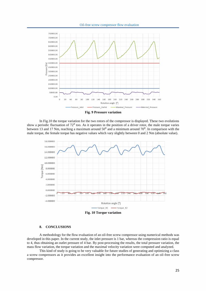
Fig. 9 shows the pressure variation for a 360⁰ rotation of the oil-free screw compressor. However,
there are two constant evolutions at 1 bar and 4 bar which corresponds to the inlet pressure and the outlet
pressure respectively. Both the minimal and the maximal pressure show a periodic evolution of 72⁰ within a
complete rotation. The maximum pressure is around 6.5 bar at 50⁰, whereas the minimum pressure values are
recorded below 0.5 bar between 15⁰ and 40⁰.
Oil-free screw compressor flow evaluation
25
Fig. 9 Pressure variation
In Fig.10 the torque variation for the two rotors of the compressor is displayed. These two evolutions
show a periodic fluctuation of 72⁰ too. As it operates in the position of a driver rotor, the male torque varies
between 13 and 17 Nm, reaching a maximum around 50⁰ and a minimum around 70⁰. In comparison with the
male torque, the female torque has negative values which vary slightly between 0 and 2 Nm (absolute value).
Fig. 10 Torque variation
8. CONCLUSIONS
A methodology for the flow evaluation of an oil-free screw compressor using numerical methods was
developed in this paper. In the current study, the inlet pressure is 1 bar, whereas the compression ratio is equal
to 4, thus obtaining an outlet pressure of 4 bar. By post-processing the results, the total pressure variation, the
mass flow variation, the torque variation and the maximal velocity variation were computed and analyzed.
This kind of study is going to be very valuable for future studies of generating and optimizing a class
a screw compressors as it provides an excellent insight into the performance evaluation of an oil-free screw
compressor.

M. GALL, V.A. POPA, I. MALAEL
26
ACKNOWLEDGEMENT
This work was carried out within “Nucleu” Program TURBO 2020, supported by the Romanian
Minister of Research and Innovation, project number PN 18.10.03.01
REFERENCES
[1] S. Kennedy, M. Wilson, S.Rane, Numerical Analysis of an Oil-free Twin Screw Compressor Using 3D
CFD and 1D Multi-chamber Thermodynamic Model, City, University of London, 10th International
Conference on Compressors and their Systems, 2017;
[2] Olly Dmitriev, Prof. Ian MacDonald Arbon, Comparison of energy-efficiency and size of portable oil-free
screw and scroll compressors, Vert Rotors UK Ltd, Edinburgh, United Kingdom, 10th International
Conference on Compressors and their Systems, 2017;
[3] Kovacevic A., Stošic N. and Smith I. K., (2007). Screw compressors - Three dimensionalcomputational
fluid dynamics and solid fluid interaction, ISBN 3-540-36302-5, Springer-Verlag Berlin Heidelberg New
York;
[4] Kovacevic A., 2002. 'Three-Dimensional Numerical Analysis for Flow Prediction in PositiveDisplacement
Screw Machines', Ph.D. Thesis, School of Engineering and MathematicalSciences, City University
London;
[5] https://www.twinmesh.com/twinmesh-features/;
[6] S.Rane, A.Kovasevic, N.Stosic, CFD Analysis of Oil Flooded Twin Screw Compressors, City University
London, Centre for Compressor Technology, London, EC1V 0HB, UK, July 2016;
[7] I.Mălăel, M.Sima, Numerical investigation of a screw compressor performance, Turbo Scientific Journal
[8] H. Ding, Y. Jiang, CFD simulation of a screw compressor with oil injection, 10th International Conference
on Compressors and their Systems, 2017;
[9] S. Rane, A. Kovacevic, N. Stosic, M. Kethidi, Grid deformation strategies for CFD analysis of screw
compressors, City University London, Centre for Positive Displacement Compressor Technology,
LondonInternational Journal of Refrigeration 36 (2013);
[10] A. Kovacevic, N. Stosic, I.K. Smith, Numerical simulation of fluid flow and solid structure in screw
compressors, Proceedings of ASME Congress, New Orleans, 2002;
[11] A.Kovacevic, N.Stosic, I.K. Smith, Three dimensional numerical analysis of screw compressor
performance,International Journal for Computational Methods in Engineering Science and Mechanics.

TURBO, vol. V (2018), no. 2
27
THE INFLUENCE OF NATURAL GAS
COMPOSITION ON SCREW COMPRESSOR OIL
Mihaiella CRETU1, Radu MIREA1
ABSTRACT: A comparative research regarding the influence of natural gas composition on screw compressor
oil was carried out in order to establish the optimal maintenance program of COMOTI’s already installed screw
compressors. Thus, samples from two different natural gas extraction sites were analysed in order to assess the
oil degradation degree. Functional analysis as flash point and cinematic viscosity have been made but also
structural analysis - FTIR was carried out in order to determine the chemical transformations that occured
during the compressor’s work. The chosen oil is XT 100 compressor oil, which is a mineral base oil.
Working in chemically, aggressive, wet gases and under special conditions for the operation of screw
compressors, a mineral base oil is affected both related to base characteristics and inner structure. The
degradation tendency of the oil is currently under analysis.
KEYWORDS: screw compressor, lubrication, oil degradation, FTIR
NOMENCLATURE
PAO – polyalphaolefin
PAG – polyalkylene glycol
PI – flash point
IR – infrared
FTIR – Fourier Transform Infrared Spectroscopy
1. INTRODUCTION
Machine conditioning monitoring or predictive maintenance is a practice of assessing a machine's
condition by periodically gathering data on machine-health indicators to determine when to schedule
maintenance. Knowing to interpret changing lubricants properties can increase both the uptime and the life of
equipment.
Lubricants are the life blood of wetted machinery. As an important element of predictive maintenance
technologies, in-service oil analysis, can provide trace information about machinery wear condition, lubricant
contamination and as well as lubricant condition. The immediate benefits of in-service oil analysis include
avoiding oil mix up, contamination control, condition based maintenance and failure analysis [1].
What is specific worldwide for the operation of a screw compressor is that oil is continuously injected
into the compressor, both to cool the gas during compression and to lubricate and cool the compressor’s parts,
while the most important characteristics required for oil are viscosity, density, flash point, foaming
characteristics and acid number [2]. Any lubricant/oil contains the so-called “base oil” (75-85% of the end
product) and a set of additives (15-25%) used to enhance the performance of the base oil and to eliminate
adverse properties that can be generated during exploitation [3].
In order to keep a rigorous eye on the operation of the industrial plants, specific sampling strategies
are in place (points along critical routes) and regular specific tests are performed [4], [5].
Lubricant is a critical component in rotary screw compressors. Understanding the characteristics of lubricant
1Romanian Research and Development Institute for Gas Turbines COMOTI, Bucharest, Romania

M. CRETU, R. MIREA
28
types helps ensure their proper application and increases customer satisfaction by extending the service life of
compressors There are many types of lubricants used in screw compressors today.
Mineral oils (petroleum oils) have long been used in various types of compressors. With oil change
intervals as low as every 1000 hours, many manufacturing plants had to change eight times per year. An
advantage of frequent oil changes is that contaminants in the compressor are removed with the waste oil.
Mineral oils have the disadvantage of a complex mix of natural hydrocarbon molecules. There are waxes that
solidify at low temperatures, volatile components that vaporize and natural mineral oils tend to quickly oxidize,
forming varnish and sludge, when exposed to high temperatures and elevated pressures.
Synthetic hydrocarbon lubricants are engineered for particular applications. For compressor
applications, polyalphaolefin (PAO) based oil is commonly used, PAO provide many of the best lubricating
features of a mineral oil and without its drawbacks. Although PAO components are derived from petroleum
base stock, they are chemically re-engineered to have a consistent, controlled molecular structure of fully
saturated hydrogen and carbon. PAO separate water extremely well, are chemical stabile and have low toxicity.
PAOs, however, are good solvents. The additive chemistry must be adjusted for this fact.
Polyglycol fluids, sometimes called PAG fluids (polyalkylene glycol), were first developed for natural
gas compressors. They were developed to reduce complaints about poor lubricant life and varnish deposits.
The formation of varnish is an indication of a petroleum or PAO lubricant that has failed. Since polyglycols do
not form varnish, there is no visual indication that the lubricant has failed. Polyglycols attract water and mix
readily. This characteristic makes separation from condensate difficult and reduces their ability to protect
bearings. The saturation point for these lubricants is much higher than for mineral or synthetic hydrocarbon
fluids, but water entrained in the fluid beyond this point will separate into free water [6].
INCDT COMOTI is currently an important producer of natural gas compression groups, equipped
with oil injection screw compressors. These equipments are difficult to implement because of the wide range
of natural gas intake parameters: the chemically and abrasively aggressive gases, wet gases, as well as the very
rigorous gas parameters at the compressor outlet. For these reasons COMOTI recomend the use of a synthetic
oil, but they are more expensive than mineral oils and the users often choose a cheaper alternative.
According to Anderol, [7], selecting the correct lubrication oil not only increases the life of a machine,
it also lowers maintenance costs and enhances the safety, productivity and reliability of the whole plant. How
an operator can achieve “correct lubrication” of a compressor depends on the importance this operator gives to
a series of factors such as cost, environment, maintenance, safety, productivity, purity of the product and other
variables.
2. PAPER CONTENT
2.1. Determination of basic oil characteristics
The aim of the paper is to test within the laboratory the oil samples from 4 screw compressors which
works in two different natural gas extraction sites. The only aspect that differenciates these locations is natural
gas composition. The used oil type from these locations is a mineral one and the 4 samples were analysed in
order to assess the oil degradation degree.
Were analyzed oil’s basic characteristics and structural analysis by FTIR method.
Altough the chosen locations for performing the experiments are situated far one from each other, the
main extraction site characteristics are similar. Thus, the compressor’s capacity, refuel pressure, working
tempersture are the same. The gas composition is different, as shown in table 1, leading to different influence
on compressor’s oil.
As it can be seen in table 1, the gas analysis for location 1 indicates that the concentration of “heavy”
C4 – C7 components is higher that for location 1. Thus, the natural gas extracted in location 1 is calles “rich”
gas. C4 – C7 components liquifies at working pressure of the compressor. Since in screw compressor, that gas
is in close contact with the oil, the liquified C4 – C7 components have a greather influence on oil’s
characteristics, primarily on viscosity and flash point.
The samples analyzed were clear but with different colours compared with the sample of new oil kept
within the laboratory, as it shown in figure 1.
Unfortunately, we don't know the working hours of the analyzed oils, but the results obtained for the
evaluated characteristics allow us to estimate the time of the oil change.

The influence of natural gas composition on screw compressor oil
29
Table 1. Gas analysis for the two locations
Location 1 Location 2
Component % vol % vol
O2 - -
N2 0.494 0.389
CO - -
CO2 0.584 1.496
CH4 97.485 97
C2H6 0.704 0.967
C3H8 0.316 0.071
i-C4H10 0.088 0.012
n-C4H10 0.137 0.01
i-C5H12 0.051 0.01
n-C5H12 0.043 0.003
C6H14 0.047 0.009
C7H16 0.051 0.033
TOTAL 100 100
Fig. 1 - Oil samples from locations 1 and 2 and fresh oil
The kinematic viscosity at 40°C and the flash point were measured in the laboratory, for each analyzed
oil sample. The obtained values for the viscosity at 40°C emphasises a 43.66-52.39 % decrease for oil used in
location 1 and 33.52-47.04 % decrease for oil used in location 2. Regarding the flash point, it has been observed
a 52.17 -64.98 % decrease for the oil used in location 1 and 50.47-62.25% decrease for the oil used in location
2.
Table 2. Obtained values for basic characteristics
Determined characteristic / Sample Viscosity at 40 °C, [mm2/s] Flash point, [C]
Method SR ISO 3104-2002 ASTM D92 - 05a
Equipment SCAVINI equipment
Ubbelohde COMECTA SCAVINI equipment
Values according to technical sheet 90-110 252
Measured values for unused oil 91.91 253
Measured values for used oil
Location 1 Compressor 1 51.78 121
Compressor 2 43.75 88.6
Location 2 Compressor 1 61.1 125.3
Compressor 2 48.67 95.5
The values obtained for the basic characteristics are showing a drastic decrease, comparated to the
unused oil, but also highlights that the concentration of liquefiable components and the operating parameters
of the compressors (machine load, speed, oil and gas pressure and temperature) have a important influence on
used oil’s characteristics.

M. CRETU, R. MIREA
30
In the screw compressors, depending on the losses due to oil filtration systems, periodically, different amounts
of new oil are added. As a result, the basic characteristics of the lubricant are improved for a while. For this
reason, it is difficult to track the working hours of each used oil.
The decisive moment for the oil change is given by the correlation of these characteristics with those obtained
by the FTIR analysis, which is presented below.
2.2. FTIR tests for oil degradation
Fourier Transform infrared spectroscopy (FTIR) is a versatile tool used to detect common
contaminants, lube degradation byproducts and additives within lubricating oils. This test method is relatively
quick to perform and is capable of simultaneously detecting multiple parameters, including antioxidants, water,
soot, fuel, glycol, oil oxidation and certain additives. Since most used oil samples are complex mixtures of
thousands of different molecules, including base oil molecules, additives, oil degradation byproducts, wear
debris and contaminants, the infrared spectrum of the sample is typically complex and can be difficult to
interpret with any degree of certainty, as some wavenumbers may overlap. Despite these drawbacks, FTIR still
has great value in used oil analysis and is employed by the majority of oil analysis labs as a screening tool. [8].
The data can be gathered by regular sampling to monitor machine performance and operating
conditions. This allows the oil to be changed at optimal intervals, which has two major benefits. Costs are
reduced by carrying out the oil change only when necessary and problems are identified early, which allows
the appropriate preventative steps to be taken. [9]
IR measurements are sensitive to a number of additives, degradation products and potential contaminants that
can be found in oil. These include:
Contamination
• Soot is a by-product of incomplete combustion and, while the oil may tolerate a significant concentration of
soot, a greater than expected increase over time may clogged filters.
• The presence of water and glycol in the oil indicates a leak from the cooling system and requires urgent
attention. Water alone may be due to condensation at low operating temperatures.
Chemical degradation
• Oxidation occurs when oil is exposed to oxygen at elevated temperatures. The reaction pathways are very
complex but the end results are thickening, varnish formation and a buildup of carboxylic acids that increase
the acidity of the oil and can lead to corrosion. Oil oxidation occurs slowly as sacrificial antioxidant additives
are used up and then rapidly once the additives have been depleted.
Regular monitoring of the oil is important to allow corrective action to be taken before this sudden
increase in oxidation occurs.
• Nitric oxides are produced during combustion, and these can also oxidise the oil, producing compounds
containing nitrogen and oxygen. As with oxidation, this leads to thickening, varnish build-up and depletion of
the oil base reserve. High levels of nitro-oxidation can indicate a number of faults, such as incorrect fuel to air
ratio, incorrect spark timing, excessive loads, low operating temperatures or piston-ring blow by.
• Acidic sulphur compounds can be produced during combustion if sulphur compounds are present as impurities
or additives in the fuel or lubricant. Again, this leads to the depletion of basic additives and eventually to
corrosion.
• Synthetic oils with a polyol ester base are susceptible to hydrolysis at elevated temperatures if water is present.
The ester breakdown products also contribute to the acidity of the oil and can sometimes form crystals that
clog filters.
Additive depletion
There are numerous compounds added to oils to confer desirable functional properties. These
additives can be depleted during use, and monitoring this depletion can provide an early warning of impending
lubricant failure.
• Anti-wear additives such as zinc di-alkyl or di-aryl dithiophosphates (ZDDPs) prevent direct metal-to-metal
contact by forming a coating on metal surfaces activated by frictional heat. These additives can be depleted by
hydrolysis or oxidation, and this can result in an increase in wear rate.
• Phenolic antioxidant compounds are often used in turbine lubricants. Depletion of the antioxidant is followed
by a rapid increase in the rate of oxidation.
Parameters that can be identified by FTIR analysis are shown in the table 3, below. [10, 11]

The influence of natural gas composition on screw compressor oil
31
Table 3. Absorption wavenumbers for FTIR
Component Spectral location Measurement
Soot, Abs/cm 3800 and 1980 cm-1 Carbon load
Water ingression (for mineral oils), % 3400 cm-1 Contaminant
Oxidation (for mineral oils), Abs/cm 1720 - 1750 cm-1 Oil Degradation
Oxidation (for organic ester), Abs/cm 3540 cm-1 Oil Degradation
Oxidation (for phosphate ester), Abs/cm 815 cm-1 Oil Degradation
Sulfation, Abs/cm 1150 cm-1 Oil Degradation
Nitration, Abs/cm 1630 cm-1 Oil Degradation
Glycol ingression, Abs/cm 880, 3400, 1040, 1080 cm-1 Contaminant
Diesel fuel ingression, Abs/cm 820 - 800 cm-1 Contaminant
Gasoline fuel ingression, Abs/cm 780 - 750 cm-1 Contaminant
Jet fuel ingression, Abs/cm 795 - 815 cm-1 Contaminant
Ester Breakdown (for synthetic oils), Abs/cm 3720 - 3590 cm-1 Oil Degradation
ZDDP anti-wear/antioxidant, Abs/cm 980 cm-1 Additive depletion
Phenol inhibitors, Abs/cm 3650 cm-1 Additive depletion
The used equipment for the assesment of the degradation of the four oil samples was done with FTIR
Spectrum OilExpress Series 100, v 3.0 spectrometer provided by Perkin Elmer, specially designed for FTIR oils analysis. As is shown in table 4, after analyzing the results, it can be observed that there are major
differences between tested samples.
So, for all the four samples, the antiwear additive was consumed. Antiwear is reported as a negative
value because it represents the depletion of some chemical component. The decrease of the antiwear leads to
the appearance and growth of the chemical degradation compounds of the oil, as is shown in Table 4: oxidation,
nitration, sulfation.
There are also, contamination products: soot 1980 and soot 3800. The values of the parameters are
different for the four oil samples analyzed, but the same tendency is observed for their growth. Given these
aspects, but mainly the depletion of the additives, these oils need to be changed.
Table 4. FTIR results for Oil XT100
Analysis Location 1 Location 2
Compressor 1 Compressor 2 Compressor 1 Compressor 2
Antiwear (Acm) 0 -1,5 -0.32 -0.86
Glycol (%) 0 0 0 0
Hydroxy (A/cm) 0 0 0 0
NOx (A/cm) 1.39 1.96 0.8 2.11
NOx vs Oxide (A/cm) 4.06 4.9 2.58 5.67
Oxidation (A/cm) 1.75 2.04 1.76 1.89
Soot 1980 (A/cm) 2.73 2.29 0 0
Soot 3800 (A/cm) 5.24 4.99 1.04 1.23
Sulf vs Oxd (A/cm) 5.89 6.77 4.89 12.27
Sulphate (A/cm) 0 0 0 0
Water (%) 0 0 0 0
The speed of IR measurement and the value and diversity of the results it provides have led to it
becoming a routine method for oil analysis labs. The figures 2, 3, 4 and 5 show the infrared spectra
of the oils analyzed compared to the reference oil (fresh oil) and the difference between them. From
this difference, with Spectrum OilExpress specific software, the data in Table 4 was obtained.
Due to the special working conditions of screw compressors and aggressive compressed gas
compositions, it is necessary to select the oil suitable for the equipment and application from each
location, and it is strictly necessary to periodically analyze the oils used to determine the working
life of the lubricant.
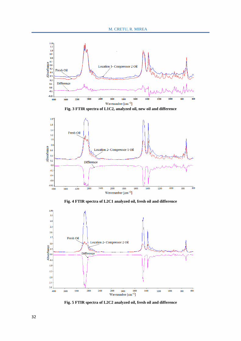
M. CRETU, R. MIREA
32
Fig. 3 FTIR spectra of L1C2, analyzed oil, new oil and difference
Fig. 4 FTIR spectra of L2C1 analyzed oil, fresh oil and difference
Fig. 5 FTIR spectra of L2C2 analyzed oil, fresh oil and difference

The influence of natural gas composition on screw compressor oil
33
3. CONCLUSIONS
• Due to the particular operating conditions of screw compressors and aggressive compressed gas
compositions, lubricating oils can be contaminated with different components, ingested or generated by the
system or may undergo oxidative degradation and decomposition of base oil and/or additives;
• Lubricant is one of the key elements in determining the service life of a rotary screw compressor;
• The gas which has a higher concentration of gasolines has a bigger influence on oil’s characteristic
and performance of mineral oils, thus this oils need to be changed more often;
• XT 100 witch is a mineral oil and has a high compatibility with gasolines, so has a decreasing of
viscosity and flash point. During screw compressor operation, chemical degradation products and contaminants
also occur;
• The specialty literature shows that each of the used oils has their advantages and drawbacks: mineral
oils can be used in less aggressive environments, PAO oils have the advantages of mineral oils but not their
drawbacks and they are more expensive then mineral oils. PAGs have the most advantages and can be used in
different locations but they are more expensive than PAO;
• In the next researches we aim to study the comparative characteristics of these three types of oils,
during the screw compressors operation.
AKNOWLEDGEMENTS
The research has been carried out within Program Nucleu TURBO 2020, project PN 16.26.06.06, financed by
Romanian Ministry of Research and Innovation.
REFERENCES
[1] WU X., XING Z., HE Z., WANG X., CHEN W., Effects of lubricating oil on the performance of a semi-
hermetic twin screw refrigeration compressor, Applied thermal engineering, vol. 112 (2017), pp 340-351
[2] *** Physical Properties of Lubricants, Engineering Tribology, Tribology Series Vol. 24, 1993, Pp 11–57
[3] *** Componenta lubrifiantilor, http://www.xoil.ro/lubrifianti/tribologie/
[4] Vidrighin C., Strategii pentru evaluarea analitică a lubrifianţilor industriali, 2013,
http://www.ttonline.ro/autori/costin-vidrighin
[5] Vidrighin C., Programe de analiza a lubrifiantilor, 2013, http://www.ttonline.ro/autori/costin-vidrighin]
[6] WAYNE P., Basics of rotary screw compressor lubricants, www.kseser.com/whitepapers, Kaeser
Compressors, Inc. 877-586-2691
[7] Roberto Chellini, Synthetic Oil vs., Mineral Oil, Compressor Tech, April 2010
[8] Wright J. Benefits of FTIR oil analysis, Machinery Lubrication, no. 8/2015
[9] Ben Perston, Raising the bar in FT-IR getting the most out of on-site oil condition monitoring, Lube
Magazine no.4 August 2011
[10] Neil Robinson, Monitoring Oil Degradation With Infrared Spectroscopy, Practicing Oil Analysis, no.11,
2007
[11] Bennett Fitch, Anatomy of an Oil Analysis Report, Machinery Lubrication, December 2015

TURBO, vol. V (2018), no. 2
34
EVALUATION OF FATIGUE BEHAVIOR ON
CARBON FIBER/EPOXY COMPOSITE
LAMINATES AT ROOM TEMPERATURE
Raluca MAIER1
ABSTRACT: Investigation of low-cycle fatigue of composites is of vital importance for the design of
structural components. In this study, Low cycle fatigue behaviour of a CFR epoxy composite was investigated
under sinusoidal wave loading at constant amplitude, a frequency of 8 Hz and stress ration R of 0.1.
Furthermore, present study experimental results were ploted on S-N diagram and compared with relevant
literature data, showing an incresed in fatigue resistance. It is found that the reinforcement architecture of the
composite material has an important influence on the fatigue life performances, when two materials are tested
in the same conditions. Likewise, it was found that an increase in apllied frequency can lead to lower fatigue
life since energy dissipated in the laminate cause heating that can reach the glass transition temperature Tg,
inducing structural degradation.
KEYWORDS: Polymer-matrix composites (PMCs), Low cycle fatigue, technology, S-N diagram
1. INTRODUCTION
Composites are nowadays an alternative, to traditional materials like metals, because of their
high stiffness and strength, low weight and adjustable properties. Carbon–fibre-reinforced polymer
matrix composites (CFRPs), for example, have been widely used for aerospace components, sporting
goods, structural applications in automobiles, ships, aircraft, etc., as consequence of their beneficial
characteristics, such as stability, high specific strength, stiffness and good chemical resistance.
Particularity in the automotive and aerospace industries the use of these materials is associated with
structural weight reduction and the consequential fuel saving and improved performance [1].
The full potential of composites as advanced materials can be realized only if the
deterioration of long-term material properties can be properly understood and controlled. In service,
composite structures are often subjected not only to static and impact loads but also to fatigue loads.
Composite materials are known to show significant darnage tolerance under dynamic loading. This
is attributed in part to the high strength and high modulus of fibers, and in part to the unique structure
of composites.
Poor fatigue performance may significantly reduce the weight advantage of many
composites. Due to their increasing use under cyclic loading conditions, fatigue studies in Carbon
Fiber Reinforced Plastics (CFRPs) have been a focus of considerable attention in recent decades.
Fatigue is the weakening or failure of a material resulting from prolonged stress. However, it is
understood that when a mass is repeatedly cyclically loaded at a location on the material, cracks
begin to form.
Fatigue loading creates fatigue damage, which in turn decreases the in-plane mechanical
properties of the composite material (strength and stiffness). Under fatigue loads, metals exhibit one
failure mode, namely a nucleation and then the propagation of one dominant crack, until the failure
occurs. On the other hand, composites consists under cyclic loading exhibit extremely complex
sequential damage accumulation process involving several micro-damage events such as transverse
1 Romanian Research and Development Institute for Gas Turbines – COMOTI, Bucharest, Romania

R. MAIER
35
matrix cracking, ply delamination, fiber matrix debonding, fiber breakage, void growth, and
delamination. Any one or a combination of these mechanisms may lead to the reduction of the overall
modulus and strength. Therefore, fatigue failure is a progressive process during which overall
modulus and strength decrease progressively until their values can no longer resist the applied
loading, and hence total failure occurs.
2. EXPERIMENTAL APPROACH
2.1. Materials and procedures
Carbon fiber fabric/epoxy (CF/E) prepreg having M49 specification (Hexcel Co) was used for the
composite preparation. In this work twill2x2 weave fabric style was used. The M49 epoxy system was
priviossely experimentaly characterized showing a 1.18g/cm3 density, a curing enthalpy of 290J/g, gel time at
120°C of 14min., a minimum viscosity of 50 poise and a Tg of 115°C after 120°C, 60 min cure dry. The
composite was prepared by using an autoclave system. The composite (3k) carbon fiber content was 58 vol%.
The composites were cured in the autoclave, under a pressure of 0.7 MPa and vacuum of 0.09 MPa, following
a heating cycle up to 120°C.
The carbon fiber/ epoxy laminates obtained (having1.47g/cm3 density) were machined using whater jet
in order to obtain experimental testing samples. Five speciments were tested for each type of regime: static
(tensile tests) and dynamic regime (Low cycle fatigue tests). Both tensile and fatigue tests were performed on
a hydraulic testing machine (Instron 8802, cell force of 150kN) according to ASTM-D3039-93 and respectively
ASTM-3479 standards. Tensile tests were carried out on 250x25x2mm±0.2 samples using 2mm/min.
desplacement rate, whereas fatigue tests were performend at different maximum stress ratios.
Stress ratio Smax (=σmin/σmax) was 0.1, where σmax and σmin are the maximum and the minimum
applied stresses, respectively, and σult is the ultimate strength of the composites. The fatigue tests were achievd
using a sinusoidal wave load at constant amplitude and a frequency of 8 Hz (the maximum frequency avaible
given by the testing device). The frequency f defines the number of repeated cycles occurring per unit time: f
= 1/T. Glass fiber/ epoxy end tabs with a length of 40 mm were attached at both ends of the specimens to avoid
failure around the gripping device during the tests. Fatigue samples geometry is presented in Fig.1. Test
conditions were monitorized (temperature 25°C, relative humidity of 45%, 4 hours of conditioning for the
sampes prior to testing).
Fig.1 Geometry and dimensions of the specimens tested in the longitudinal tensile and fatigue tests
2.2. Results and discussions
Tensile properties
The static tensile properties of carbon fiber/epoxy laminates were quoted against the literature results [5,6] in
table 1. It is necessary to mention that both present study as well as [5,6] materials are epoxy-
impregnated woven carbon fabrics. Both E. C. Botelho et al. [5] and Z. Khan et al. [6] used plain-weave woven
carbon fabrics. Within Z. Khan et al. [6] study [0˚]8 ply configuration samples cured in an autoclave at 177o C
, 8 bars. E. C. Botelho et al. [5] laminates were cured in autoclave, under a pressure of 0.69 MPa and vacuum
of 0.083 MPa, following a heating cycle up to 181oC. Present study tested specimens were bidirectional twill
2x2 [0˚]8 whereas plain weave woven fabrics [0˚]8 were used in [5], so in both cases, in 0˚ and 90˚ the load
will be almost the same.

Evaluation of fatigue behavior on carbon fiber/epoxy composite laminates at room temperature
36
Table 1. Tensile properties for composite materials under study
Material Hexply M49 Hexply F155 [5]
Tensile stress (MPa) 902±34 892 ± 4
Tensile strain (%) 0.65±0.08 0.82 ± 0.06
Elastic modulus (GPa) 69±2.5 67.2 ± 2.1
Fatigue results S-N curves
The applied fatigue stress can be expressed as the maximum fatigue stress Smax. This normalized
applied stress is the ratio of the maximum fatigue stress to the ultimate quasi-static stress or strength of the
composite. The normalized applied stress is often used to compare two or more materials with different values
of ultimate stress. In cycle fatigue, materials performance is commonly characterized by an S-N curve, also
known as a Wöhler curve. This graph of the magnitude of a cyclic stress (S) against the logarithmic scale of
cycles to failure (N) for the tested materials is presented in Fig. 2. These study experimental results are plotted
against Edson C. Botelho et al. [5] and Z. Khan et al. [6] data. It is worth reminding that this study as well as
Edson C. Botelho et al. [5] fatigue experiments were performed at Smax = 0.1 and 8 Hz frequency, whereas Z.
Khan et al. [6] fatigue results were obtained for Smax = 0.1 and 20 Hz frequency.
Fig. 2 Fatigue test results (SN curves) for present study materials compared with literature data [5,6]
According to Fig. 2, it can be observed that in low to high cycle fatigue, present study material show
an incresed fatigue resistance when compared with literature data [5], nevertheless fatigue behaviour trend
seems similar. In low cycle domain the fatigue resistance for this study carbon fiber/epoxy laminates is between
440 and 550 MPa, and in high cycles, these values are lower when compared with the ones found in low cycles,
being 275– 400 MPa. The effect of apllied frequency range (8Hz used in the present study and [5], compared
with 20Hz used in [6]) is very significant.
Likewise in the research [6] fatigue resistance of the carbon fiber/epoxy material is between 350-
400MPa in high cycle fatigue whereas in low cycle regime varies between 375-415MPa. Lower maximum
stress and higher frequency leads to different local damage mechanisms due to fatigue mechanical solicitation.
Fatigue loading can lead to energy dissipation in the laminate causing heating of the laminate. When the loading
frequency is sufficiently high such that the laminate does not have time to cool down and temperatures reach
the glass transition temperature Tg, the fatigue performance can be affected negatively, leading to lower fatigue
lives. Moreover, at lower frequencies, hysteresis effects can influence the fatigue life significantly because they
can lead to localised stress redistribution processes. Thereby, the matrix crack propagation rate can be reduced
and the fatigue life is increased.
In his PhD study A.A.R. Broer [7] reported a comparison between carbon-epoxy (AS4/8552)
laminates with cross-ply lay-up of [90/0/90]2S tested at same R ratio=0.1 and using loading frequencies of 5
and respectively 10 Hz. For each maximum stress value he reported (table 2) the fatigue life in terms of N f
(number of cycles).
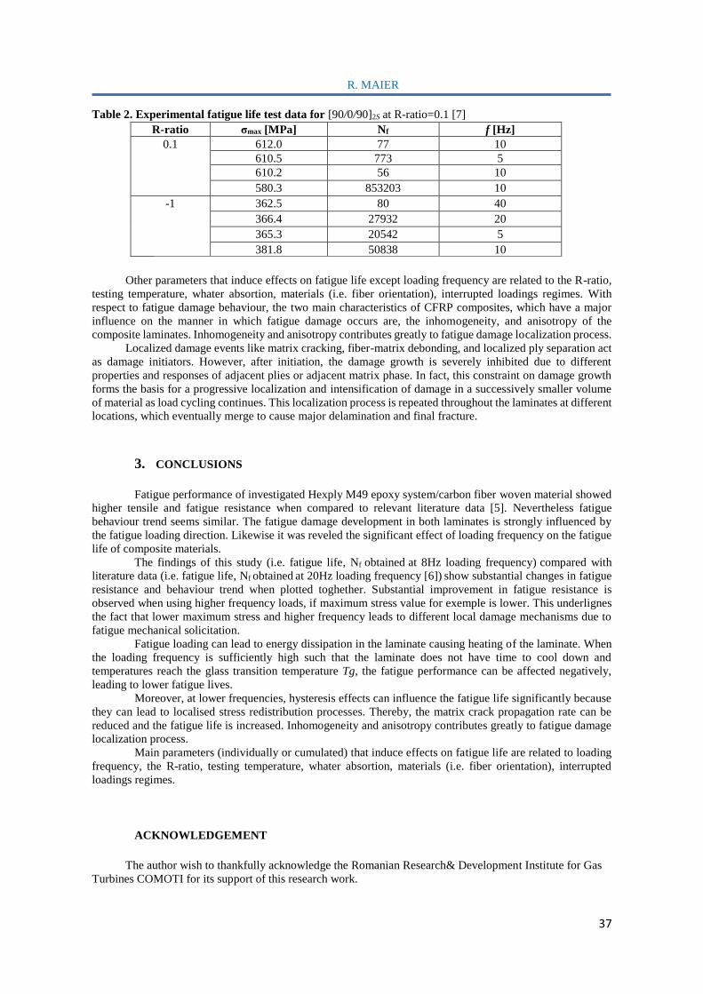
R. MAIER
37
Table 2. Experimental fatigue life test data for [90/0/90]2S at R-ratio=0.1 [7]
R-ratio σmax [MPa] Nf f [Hz]
0.1 612.0 77 10
610.5 773 5
610.2 56 10
580.3 853203 10
-1 362.5 80 40
366.4 27932 20
365.3 20542 5
381.8 50838 10
Other parameters that induce effects on fatigue life except loading frequency are related to the R-ratio,
testing temperature, whater absortion, materials (i.e. fiber orientation), interrupted loadings regimes. With
respect to fatigue damage behaviour, the two main characteristics of CFRP composites, which have a major
influence on the manner in which fatigue damage occurs are, the inhomogeneity, and anisotropy of the
composite laminates. Inhomogeneity and anisotropy contributes greatly to fatigue damage localization process.
Localized damage events like matrix cracking, fiber-matrix debonding, and localized ply separation act
as damage initiators. However, after initiation, the damage growth is severely inhibited due to different
properties and responses of adjacent plies or adjacent matrix phase. In fact, this constraint on damage growth
forms the basis for a progressive localization and intensification of damage in a successively smaller volume
of material as load cycling continues. This localization process is repeated throughout the laminates at different
locations, which eventually merge to cause major delamination and final fracture.
3. CONCLUSIONS
Fatigue performance of investigated Hexply M49 epoxy system/carbon fiber woven material showed
higher tensile and fatigue resistance when compared to relevant literature data [5]. Nevertheless fatigue
behaviour trend seems similar. The fatigue damage development in both laminates is strongly influenced by
the fatigue loading direction. Likewise it was reveled the significant effect of loading frequency on the fatigue
life of composite materials.
The findings of this study (i.e. fatigue life, Nf obtained at 8Hz loading frequency) compared with
literature data (i.e. fatigue life, Nf obtained at 20Hz loading frequency [6]) show substantial changes in fatigue
resistance and behaviour trend when plotted toghether. Substantial improvement in fatigue resistance is
observed when using higher frequency loads, if maximum stress value for exemple is lower. This underlignes
the fact that lower maximum stress and higher frequency leads to different local damage mechanisms due to
fatigue mechanical solicitation.
Fatigue loading can lead to energy dissipation in the laminate causing heating of the laminate. When
the loading frequency is sufficiently high such that the laminate does not have time to cool down and
temperatures reach the glass transition temperature Tg, the fatigue performance can be affected negatively,
leading to lower fatigue lives.
Moreover, at lower frequencies, hysteresis effects can influence the fatigue life significantly because
they can lead to localised stress redistribution processes. Thereby, the matrix crack propagation rate can be
reduced and the fatigue life is increased. Inhomogeneity and anisotropy contributes greatly to fatigue damage
localization process.
Main parameters (individually or cumulated) that induce effects on fatigue life are related to loading
frequency, the R-ratio, testing temperature, whater absortion, materials (i.e. fiber orientation), interrupted
loadings regimes.
ACKNOWLEDGEMENT
The author wish to thankfully acknowledge the Romanian Research& Development Institute for Gas
Turbines COMOTI for its support of this research work.

Evaluation of fatigue behavior on carbon fiber/epoxy composite laminates at room temperature
38
REFERENCES
[1] P.N.B. Reis, J.A.M. Ferreira, J.D.M. Costa, M.O.W. Richardson; 2009; Fatigue life evaluation for
carbon/epoxy laminate composites under constant and variable block loading; Composites Science and
Technology; Vol. 69; 154–160
[2] David Bayless; Sample Formal Laboratory Report, Fatigue Failure through Bending Experiment; Report
submitted by Sarah Thomas; Lab Partners: David Henry and James Johnson; ME 498; November 10, 2004
[3] M. Y. Mazin, N. Mallik; 2012; Low Cycle Fatigue Failure of Composite Materials/Aluminium Alloys At
Different Heat Treatments, International Journal of Scientific & Engineering Research; Vol. 3; No. 6; 1-6
[4] M. Kawai, M. Koizumi; 2007; Nonlinear constant fatigue life diagrams for carbon/epoxy laminates at room
temperature, Composites: Part A; Vol. 38; 2342–2353
[5] E. C. Botelho, M. C. Rezende, S. Mayer, H. Voorwald; 2008; Evaluation of fatigue behavior on repaired
carbon fiber/epoxy composites; Journal of Materials Science; Vol.43; 3166–3172
[6] Z. Khan, R. Khan, F. Al-Sulaiman, N. Merah; 2002; Fatigue damage in woven carbon fabric/epoxy
laminates at non-ambient temperatures; The 6th Saudi Engineering Conference, Vol. 5; KFUPM, Dhahran;
December 2002; 313
[7] A.A.R. Broer; 23 May 2018; Fatigue life prediction of carbon fibre-reinforced epoxy laminates using a
single S-N curve; Master of Science Thesis; Faculty of Aerospace Engineering; Delft University of
Technology.
TURBO, vol. V (2018), no. 2
39
HEAT TREATMENT INFLUENCE ON HARDNESS
AND MICROSTRUCTURE OF ADAM
MANUFACTURED 17-4 PH
Mihaela Raluca CONDRUZ1, Alexandru PARASCHIV1, Cristian PUSCASU1
ABSTRACT: The influence of heat treatment on the main characteristics of atomic diffusion additive
manufactured 17-4 PH stainless steel was studied. Several investigations such as chemical micro-composition,
porosity analysis, microstructural analysis and hardness measurement were done in order to assess the
properties of the steel as compared with those provided or recommended by technical data sheets for the
material produced by this additive manufacturing method. The average porosity experimentally identified was
0.128%, value lower as compared with the porosity indicated by the technical data sheet, which prove that
high-density materials can be produced by ADAM method. Microstructural SEM investigation of the as printed
steel have shown a structure formed by martensite and ferrite. After an optimized heat treatment, in quenched
state from 1050°C in air, martensite and ferrite with residual austenite at grain boundary were noticed and after
a further tempering at 450°C ferrite was revealed as well at the grain boundaries. After applying the optimized
heat treatment, an average hardness of 28HRC was obtained which is in very good agreement with the hardness
values reported for additive manufactured 17-4 PH.
KEYWORDS: 17-4PH, additive manufacturing, heat treatment, microstructure
1. INTRODUCTION
17-4 PH is a precipitation hardened steel developed for specific industrial fields (aerospace, chemical,
petrochemical, general metalworking) where it has to provide high strength and toughness while maintaining
good corrosion resistance [1]. It is a martensitic stainless steel containing approximately 3wt% Cu that ensure
the strengthening by precipitation in the martensitic matrix. Until the last decade, the main manufacturing
methods used to produce this material were conventional casting, powder metallurgy and metal injection
moulding (MIM). However, nowadays additive manufacturing (AM) is the most studied process in order to
manufacture metallic parts. It seems that in the scientific literature the most studied AM method in case of
development of dense 17-4PH parts is selective laser melting (SLM). For example, Gu et.al. [2] studied the
influence of SLM process parameters on the porosity and microstructure of 17-4PH. They observed that even
if a set of optimum parameters were established, the coupons present a significant porosity level (up to 5.4%).
Regarding the microstructure, they observed very fine, parallel columnar austenitic grains and approx. 70 vol.%
of martensite. Banerjee et.al. [3] researched the properties and microstructure of 17-4 PH obtained by MIM,
using 3 different atmospheres in case of sintering (hydrogen, nitrogen, vacuum). They didn’t obtain fully
densified samples, but in all cases the microstructure was a dendritic δ-ferrite in a martensitic matrix. The same
phases were identified by Machaka [4] in case of 17-4 PH obtained by MIM.
Murr et.al. [5] investigated the microstructures and properties of 17-4 PH manufactured by SLM using
Ar/N2 as fabrication gas. The raw material consisted in pre-alloyed 17-4 PH powders obtained by Ar or N2
atomization which resulted in a different structure: Ar-atomized powder presented a completed body centered
cubic (BCC) α-Fe while the N2-atomized powder was primarily face centered cubic (FCC) γ-Fe with 6% BCC
α-Fe. A difference was observed regarding the HRC hardness of samples, for example the hardness identified
in case of austenitic samples was approx. 21 HRC while the martensitic samples had an approx. 31 HRC with
the possibility of increasing it until approx. 41 HRC after post processing.
1 Romanian Research and Development Institute for Gas Turbines COMOTI, Bucharest, Romania

M.R. CONDRUZ, A. PARASCHIV, C. PUSCASU
40
Pasebani et.al. [6] studied the effects of atomizing environment (water vs gas) and post processing on
mechanical properties of 17-4 PH manufactured via SLM. They observed that after solutionizing at 1315ºC
and aging at 482°C, fully martensitic structure was obtained and the atomizing environment can influence the
hardness of the material. In case of specimens manufactured from water atomized powders the hardness
obtained was 40.2 HRC compared with 42.7 HRC in case of gas atomized powders and 39 HRC in case of
wrought alloy.
Irrinki et.al. [7] studied the effect of particle characteristics on the microstructure and mechanical
properties of 17-4 PH fabricated by laser-powder bed fusion. In their research, they obtained high dens parts
(97 ±0.5%) with a hardness between 25-39 HRC.
The goal of the present paper was to assess the influence of different heat treatments on hardness and
microstructure of the 17-4PH stainless steel produced by another another additive manufacturing method,
atomic diffusion additive manufacturing – ADAM.
2. EXPERIMENTAL PROCEDURE
2.1 Materials and procedures
For this study, the 17-4 PH was provided by MARKFORGED Inc. and it was obtained by ADAM
method. The manufacturers sustain that this is an industrial metal printing method that can provide metallic
parts with high speed and accuracy. This method is based on FDM method (fused deposition modeling) due to
the fact that it uses metal powders that are encased in plastic binders. During the manufacturing process, the
plastic is melted off and successive material layers are deposited, the plastic is dissolved entirely during a
washing process (a semi-porous part is obtained) and afterwards the part is sintered in an oven [8].
17-4 PH samples were cut from a rod and were metallographically prepared by grinding and polishing.
Different heat treatments were realized along with porosity analysis, microstructural investigations and
hardness determinations.
The heat treatment temperature was established based on AK Steel 17-4 PH Product Data Bulletin [9]
and it consisted in quenching at 1040˚C, maintaining for 40 minutes and air cooling to room temperature.
Afterwards samples were tempered for 90 minutes at temperatures 550°C (treatment 1), respective 450°C
(treatment 2) followed by air cooling to room temperature. The heat treatment was performed using a
Nabertherm LH 30/14 oven (P=10 kW, Tmax=1673 K).
For microstructural investigations, the samples were etched with Marble etchant (10g CuSO4, 50ml
HCl, 50ml H2O). Microstructural analysis was performed using an optic microscope and a scanning electron
microscope (SEM – FEI Inspect F50). The chemical composition analysis was performed by energy dispersive
spectrometry (EDS – EDAX) and optical emission spectroscopy (OES) using the spectrometer Foundry Master.
The porosity evolution was assessed on SEM images using image processing software Scandium by
adjusting the brightness and contrast to highlight the pores and afterwards converting the images to a 16-bit
greyscale format and conversion into black and white threshold images. The analysis was realized on 10
different areas from the samples. The phase proportions were determined by using Schaeffler diagram and
chemical composition determined by EDS – EDAX in multiple areas of the samples.
Brinell hardness was determined before and after the heat treatment. The tests were realized using
EMCO TEST M4C/R 025G3M according to ASTM E10 – 17 [10] (50 mm ball, indentation force 62 kg), four
measurements were made and an average hardness value was presented.
2.2 Results and discussions
Chemical composition analysis
The chemical composition experimentally determined was compared with standard composition of
cast alloy and composition provided by the technical data sheet of ADAM manufactured 17-4 PH [11]. Table
1 presents the chemical composition of 17-4 PH. It can be observed that the experimentally determined
chemical compositions fall in the theoretical predictions for this alloy. Figure 1 presents the EDS spectrum
obtained for 17-4 PH.
Comparing the chemical composition experimentally determined with the theoretical chemical
composition it can be said that the EDS analysis results are in a good agreement with the data provided by the
technical data sheet. In case of OES analysis differences were encountered in case of the elements that are in a
small proportion.

Heat treatment influence on hardness and microstructure of ADAM manufactured 17-4PH
41
Fig. 1 Micro-area used for chemical analysis by EDS and EDS spectrum obtained
Table 1. Chemical composition of 17-4 PH
Alloy state Elements [wt.%]
C Mn P S Si Cr Ni Cu N Nb+Ta Fe
Cast [9] max.
0.07
max.
1.00
max
0.04
max.
0.03
max.
1.00
15.00
-
17.50
3.00
-
5.00
3.00
-
5.00
- 0.15 -
0.45
Bal.
ADAM
[11]
max.
0.07
max.
1.00
max
0.04
- 0.5 -
1.00
15.00
-
17.50
3.00
-
5.00
3.00
-
5.00
- 0.15 -
0.45
Bal.
ADAM
determined
by EDS
0.05 0.98 0.03 - 1.05 15.99 3.95 3.9 - 0.27 Bal.
ADAM
determined
by OES
0.02 0.13 0.003 - 0.23 15.9 4.63 3.76 - 0.04 Bal.
Porosity analysis
Additive manufactured materials are characterized by different degree of porosity. The porosity is
caused mainly by the manufacturing method used and the process parameters selection. Moreover, porosity
can be a result from microfractures or shrinkage cavities. In Figure 2 can be observed an example of binarized
SEM image used for porosity analysis.
Fig. 2 Binarized SEM image used for porosity analysis
The average porosity experimentally identified for ADAM manufactured 17-4 PH was 0.128%. It
was observed that this degree of porosity is lower than the degree indicated in the technical data sheet (2-4%)
which proves that high-density materials can be obtained by ADAM method.
Microstructural analysis
Figure 3 present the ADAM 17-4 PH microstructure in the initial state and after heat treatment, images
obtained after etching. From optical microscopy images can be observed that before the heat treatment a major
phased was identified – acicular martensite which also appears after heat treatment 1 and heat treatment 2 were
applied, but its proportion was reduced after appling the second heat treatment.

M.R. CONDRUZ, A. PARASCHIV, C. PUSCASU
42
a b c
Fig. 3 Optic microscopy with ADAM 17-4 PH alloy microstructure: a) as printed state; b) material
after treatment 1; c) material after treatment 2
Figures from 4 to 7 present SEM images with the microstructure of the material in different states: as
printed state, quenched state, after quenching and tempering at 550˚C and after quenching and tempering at
450˚C/90min. Two different phases can be observed in the SEM images, an acicular majority phase and small
quantities of a second phase disposed at the grain boundaries, between the acicular phase.
Based on chemical composition obtained by EDS in different areas of the samples, and using the
Schaffler diagram (Figure 8) were determined the phase proportions in different states of the material: as
printed state, quenched state and after quenching and tempering at 450˚C.
Fig. 4 SEM images with ADAM 17-4 PH material in as printed state
Fig. 5 SEM images with ADAM 17-4 PH material after quenching from 1040˚C/40min
Fig. 6 SEM images with ADAM 17-4 PH material after quenching from 1040˚C/40min and tempering
at 550˚C/90min

Heat treatment influence on hardness and microstructure of ADAM manufactured 17-4PH
43
Fig. 7 SEM images with ADAM 17-4 PH material after quenching from 1040˚C/40min and tempering
at 450˚C/90min
Fig. 8 Schaeffler diagram used to determine stainless steel phases
Based on the qualitative chemical composition of the material determined by EDS, the following
phases were identified:
- in the as printed state martensite and ferrite were observed (majority phases identified also by
Schroeder et.al. [12] in case of 17-4 PH obtained by plasma debinding and sintering);
- in the quenched state the material presented martensite and ferrite with the addition of austenite at the
grain boundary;
- after quenching and tempering at 450°C the same three phases were identified with the difference that
at the grain boundaries ferrite was encountered along with austenite. This could be a result of different
carbon content (lower carbon content could result in an increase of δ-ferrite quantity).
Hardness
Table 2 presents the hardness values determined for ADAM manufactured 17-4 PH before and after
heat treatments were applied. The values were compared with the average hardness of cast 17-4 PH.
Table 2. Hardness identified for 17-4 PH
Material state HBW 5/62.5
Cast 274
As printed 240
Quenching from1040˚C/40min in air 260
Quenching from 1040˚C/40min in air + tempering at
550˚C for 90min
261
Quenching from 1040˚C/40min in air + tempering at
450˚C for 90min
271
M.R. CONDRUZ, A. PARASCHIV, C. PUSCASU
44
From the registered values it can be observed that in the as printed state, 17-4 PH presents a lower
hardness compared with the value of the cast material, but after the proper heat treatment was applied the
hardness improved and was significant higher compared with the as printed state, and close to the cast hardness
(271 HBW 5/62 – approx. 28 HRC vs. 274 HBW 5/62 approx. 28.8 HRC).
In the literature, multiple results were identified regarding the hardness of 17-4 PH manufactured by
other methods, but the ADAM manufactured 17-4 PH hardness is included in the range encountered in the
literature 21 - 42.7 HRC.
3. CONCLUSIONS
The present study was focused on determination of heat treatment influence on microstructure and
hardness of 17-4 PH stainless steel obtained by ADAM method. It represents the first step towards evaluating
the possibility of manufacturing parts of 17-4 PH by this AM method.
The chemical composition determined was in a good agreement with the chemical composition
provided by the technical data sheet. The average porosity experimentally identified was 0.128%, value lower
compared with the porosity indicate by the technical data sheet, which prove that high-density materials can
be obtained by ADAM method.
Similar phases were identified in ADAM manufactured 17-4 PH as in plasma debinding and sintering
manufactured 17-4 PH. Based on the qualitative chemical composition of the material determined by EDS, in
the as printed state martensite and ferrite were observed, in the quenched state the material presented martensite
and ferrite with the addition of austenite at the grain boundary and after quenching and tempering at 450°C the
same three phases were identified with the difference that at the grain boundaries ferrite was encountered along
with austenite.
It was observed that in as printed state, 17-4 PH presents a lower hardness compared with the value
of the cast material, but after the proper heat treatment was applied the hardness improved and was significant
higher compared with the as printed state, and close to the cast hardness (271 HBW 5/62 – approx. 28 HRC
vs. 274 HBW 5/62 approx. 28.8 HRC). The hardness of ADAM manufactured 17-4 PH is in the range identified
in the literature (21-42.7 HRC).
Future investigations will be realized in order to characterize the material 17-4 PH manufactured by
ADAM and to determine the suitability of ADAM technology for manufacturing rotary components.
ACKNOWLEDGEMENT
This paper was realized within Nucleu Program TURBO 2020+ with the help of Minister of Research and
Innovation (MCI), the project number PN 18.10.02.02. The authors would like to thank to Micheal Goodwin
and Tom Cannon from MARKFORGED Inc. for providing the material used in the investigations.
REFERENCES
[1] Murathan, O.F., Abul, M.R.; 2012; Heat Treatment of 17-4 PH Stainless Steel, Term Project; Atilim
University, Turkey
[2] Gu, H., Gong, H., Pal, D., Starr, T., Stucker, B.; 2013; Influences of Energy Density on Porosity and
Microstructure of Selective Laser Melted 17-4PH Stainless Steel; 24th Annual International Solid Freeform
Fabrication Symposium
[3] Banerjee, S., Joens, C.J.; 2008; A Comparison of Techniques for Processing Powder Metal Injection
Molded 17-4 PH Materials; Web-site:
http://www.dshtech.com/pub/files/Comparisonoftechniquesforprocessingpowermetalinjectionmolded.pdf
[4] Machaka, R.; 2018; Metal injection moulding of a 17-4 PH stainless steel: a comparative study of
mechanical properties; IOP Conf. Series: Materials Science and Engineering, 430, 012033, doi:10.1088/1757-
899X/430/1/012033
[5] Murr, L.E., Martinez, E., Hernandez, J., Collins, S., Amato, K.N., Gaytan, S.M., Shindo, P.W.; 2012;
Microstructures and Properties of 17-4 PH Stainless Steel Fabricated by Selective Laser Melting, Journal of
Material Research and Technology, 1 (3), pp. 167-177

Heat treatment influence on hardness and microstructure of ADAM manufactured 17-4PH
45
[6] Pasebani, S., Ghayoor, M., Badwe, S., Irrinki, H., Atre, S.V.; 2018; Effects of atomizing media and post
processing on mechanical properties of 17-4 PH stainless steel manufactured via selective laser melting,
Additive Manufacturing, 32, pp. 127-137, https://doi.org/10.1016/j.addma.2018.05.011
[7] Irrinki, H., Jangam, J.S.D., Pasebani, S., Badwe, S., Stitzel, J., Kate, K., Gulsoy, O., Atre, S.V.; 2018;
Effects of particle characteristics on the microstructure and mechanical properties of 17-4 PH stainless steel
fabricated by laser-powder bed fusion, Powder Technology, 331, pp. 192-203, 2018,
https://doi.org/10.1016/j.powtec.2018.03.025
[8] Web-site: https://3dprinting.com/metal/atomic-diffusion-additive-manufacturing-game-changer/
[9] 17-4 PH-B-08-01-07: 17-4 PH Stainless steel product data bulletin, AK Steel
[10] Material Specification 17-4 PH Stainless steel, Markforged Inc. Data sheet, Rev 1.0 – 1/1/2018
[11] ASTM E10 – 17: Standard Test Method for Brinell Hardness of Metallic Materials
[12] Schroeder, R, Hammes, G., Binder, C., Klein, A.N.; 2011; Plasma debinding and sintering of metal
injection moulded 17-4PH stainless steel, Mat. Res., 14(4), http://dx.doi.org/10.1590/S1516-
14392011005000082