ML. Numerical Methods - deliu.ro numerice.pdf · ML.1 Numerical Methods in Linear Algebra ML.1.1...
142
Contract POSDRU/86/1.2/S/62485 Universitatea Tehnic˘ a din Cluj-Napoca Ioan Gavrea Mircea Ivan ML. Numerical Methods Universitatea Tehnic˘ a ”Gheorghe Asachi” din Ia¸ si Universitatea din Craiova
Transcript of ML. Numerical Methods - deliu.ro numerice.pdf · ML.1 Numerical Methods in Linear Algebra ML.1.1...
Contract POSDRU/86/1.2/S/62485
Universitatea Tehnica din Cluj-Napoca
Ioan Gavrea Mircea Ivan
ML. Numerical Methods
Universitatea Tehnica
”Gheorghe Asachi” din Iasi
Universitatea
din Craiova

Contents
ML.1 Numerical Methods in Linear Algebra 7
ML.1.1 Special Types of Matrices . . . . . . . . . . . . . . . . . . . . . . . . . . . 7
ML.1.2 Norms of Vectors and Matrices . . . . . . . . . . . . . . . . . . . . . . . . 9
ML.1.3 Error Estimation . . . . . . . . . . . . . . . . . . . . . . . . . . . . . . . . 14
ML.1.4 Matrix Equations. Pivoting Elimination . . . . . . . . . . . . . . . . . . . 16
ML.1.5 Improved Solutions of Matrix Equations . . . . . . . . . . . . . . . . . . . 20
ML.1.6 Partitioning Methods for Matrix Inversion . . . . . . . . . . . . . . . . . . 20
ML.1.7 LU Factorization . . . . . . . . . . . . . . . . . . . . . . . . . . . . . . . . 23
ML.1.8 Doolittle’s Factorization . . . . . . . . . . . . . . . . . . . . . . . . . . . . 28
ML.1.9 Choleski’s Factorization Method . . . . . . . . . . . . . . . . . . . . . . . . 31
ML.1.10 Iterative Techniques for Solving Linear Systems . . . . . . . . . . . . . . . 33
ML.1.11 Eigenvalues and Eigenvectors . . . . . . . . . . . . . . . . . . . . . . . . . 36
ML.1.12 Characteristic Polynomial: Le Verrier Method . . . . . . . . . . . . . . . . 38
ML.1.13 Characteristic Polynomial: Fadeev-Frame Method . . . . . . . . . . . . . . 39
ML.2 Solutions of Nonlinear Equations 41
ML.2.1 Introduction . . . . . . . . . . . . . . . . . . . . . . . . . . . . . . . . . . . 41
ML.2.2 Method of Successive Approximation . . . . . . . . . . . . . . . . . . . . . 42
ML.2.3 The Bisection Method . . . . . . . . . . . . . . . . . . . . . . . . . . . . . 43
ML.2.4 The Newton-Raphson Method . . . . . . . . . . . . . . . . . . . . . . . . . 44
ML.2.5 The Secant Method . . . . . . . . . . . . . . . . . . . . . . . . . . . . . . . 45
ML.2.6 False Position Method . . . . . . . . . . . . . . . . . . . . . . . . . . . . . 45
ML.2.7 The Chebyshev Method . . . . . . . . . . . . . . . . . . . . . . . . . . . . 46
ML.2.8 Numerical Solutions of Nonlinear Systems of Equations . . . . . . . . . . . 48
ML.2.9 Newton’s Method for Systems of Nonlinear Equations . . . . . . . . . . . . 49
ML.2.10 Steepest Descent Method . . . . . . . . . . . . . . . . . . . . . . . . . . . 51
ML.3 Elements of Interpolation Theory 53
ML.3.1 Lagrange Interpolation . . . . . . . . . . . . . . . . . . . . . . . . . . . . . 53
ML.3.2 Some Forms of the Lagrange Polynomial . . . . . . . . . . . . . . . . . . . 54
ML.3.3 Some Properties of the Divided Difference . . . . . . . . . . . . . . . . . . 61
ML.3.4 Mean Value Properties in Lagrange Interpolation . . . . . . . . . . . . . . 63
3
4 CONTENTS
ML.3.5 Approximation by Interpolation . . . . . . . . . . . . . . . . . . . . . . . . 65
ML.3.6 Hermite-Lagrange Interpolating Polynomial . . . . . . . . . . . . . . . . . 65
ML.3.7 Finite Differences . . . . . . . . . . . . . . . . . . . . . . . . . . . . . . . . 68
ML.3.8 Interpolation of Functions of Several Variables . . . . . . . . . . . . . . . . 71
ML.3.9 Scattered Data Interpolation. Shepard’s Method . . . . . . . . . . . . . . . 72
ML.3.10 Splines . . . . . . . . . . . . . . . . . . . . . . . . . . . . . . . . . . . . . . 74
ML.3.11 B-splines . . . . . . . . . . . . . . . . . . . . . . . . . . . . . . . . . . . . . 75
ML.3.12 Problems . . . . . . . . . . . . . . . . . . . . . . . . . . . . . . . . . . . . 78
ML.4 Elements of Numerical Integration 81
ML.4.1 Richardson’s Extrapolation . . . . . . . . . . . . . . . . . . . . . . . . . . 81
ML.4.2 Numerical Quadrature . . . . . . . . . . . . . . . . . . . . . . . . . . . . . 82
ML.4.3 Error Bounds in the Quadrature Methods . . . . . . . . . . . . . . . . . . 83
ML.4.4 Trapezoidal Rule . . . . . . . . . . . . . . . . . . . . . . . . . . . . . . . . 84
ML.4.5 Richardson’s Deferred Approach to the Limit . . . . . . . . . . . . . . . . 85
ML.4.6 Romberg Integration . . . . . . . . . . . . . . . . . . . . . . . . . . . . . . 86
ML.4.7 Newton-Cotes Formulas . . . . . . . . . . . . . . . . . . . . . . . . . . . . 87
ML.4.8 Simpson’s Rule . . . . . . . . . . . . . . . . . . . . . . . . . . . . . . . . . 88
ML.4.9 Gaussian Quadrature . . . . . . . . . . . . . . . . . . . . . . . . . . . . . . 88
ML.5 Elements of Approximation Theory 91
ML.5.1 Discrete Least Squares Approximation . . . . . . . . . . . . . . . . . . . . 91
ML.5.2 Orthogonal Polynomials and Least Squares Approximation . . . . . . . . . 93
ML.5.3 Rational Function Approximation . . . . . . . . . . . . . . . . . . . . . . . 95
ML.5.4 Pade Approximation . . . . . . . . . . . . . . . . . . . . . . . . . . . . . . 95
ML.5.5 Trigonometric Polynomial Approximation . . . . . . . . . . . . . . . . . . 97
ML.5.6 Fast Fourier Transform . . . . . . . . . . . . . . . . . . . . . . . . . . . . . 99
ML.5.7 The Bernstein Polynomial . . . . . . . . . . . . . . . . . . . . . . . . . . . 101
ML.5.8 Bezier Curves . . . . . . . . . . . . . . . . . . . . . . . . . . . . . . . . . . 106
ML.5.9 The METAFONT Computer System . . . . . . . . . . . . . . . . . . . . . 107
ML.6 Integration of Ordinary Differential Equations 109
ML.6.1 Introduction . . . . . . . . . . . . . . . . . . . . . . . . . . . . . . . . . . . 109
ML.6.2 The Euler Method . . . . . . . . . . . . . . . . . . . . . . . . . . . . . . . 109
ML.6.3 The Taylor Series Method . . . . . . . . . . . . . . . . . . . . . . . . . . . 110
ML.6.4 The Runge-Kutta Method . . . . . . . . . . . . . . . . . . . . . . . . . . . 111
ML.6.5 The Runge-Kutta Method for Systems of Equations . . . . . . . . . . . . . 112
ML.7 Integration of Partial Differential Equations 115
ML.7.1 Introduction . . . . . . . . . . . . . . . . . . . . . . . . . . . . . . . . . . . 115
ML.7.2 Parabolic Partial-Differential Equations . . . . . . . . . . . . . . . . . . . 116

CONTENTS 5
ML.7.3 Hyperbolic Partial Differential Equations . . . . . . . . . . . . . . . . . . . 116
ML.7.4 Elliptic Partial Differential Equations . . . . . . . . . . . . . . . . . . . . . 117
ML.7 Self Evaluation Tests 119
ML.7.1 Tests . . . . . . . . . . . . . . . . . . . . . . . . . . . . . . . . . . . . . . . 119
ML.7.2 Answers to Tests . . . . . . . . . . . . . . . . . . . . . . . . . . . . . . . . 124
Index 136
Bibliography 139

6
ML.1
Numerical Methods in Linear Algebra
ML.1.1 Special Types of Matrices
LetMm,n(R) be the set of all m×n type matrices with real entries, where m,n are positiveintegers (Mn(R) :=Mn,n(R)).
DEFINITION ML.1.1.1
A matrix A ∈ Mn(R) is said to be strictly diagonally dominant when its entriessatisfy the condition
|aii| >n∑
j=1j 6=i
|aij|
for each i = 1, . . . , n.
THEOREM ML.1.1.2
A strictly diagonally dominant matrix is nonsingular.
Proof. Consider the linear system
AX = 0, A ∈Mn(R),
which has a nonzero solution X = [x1, . . . , xn]t ∈Mn,1(R). Let k be an index such that
|xk| = max1≤j≤n
|xj|.
Sincen∑
j=1
akjxj = 0,
7
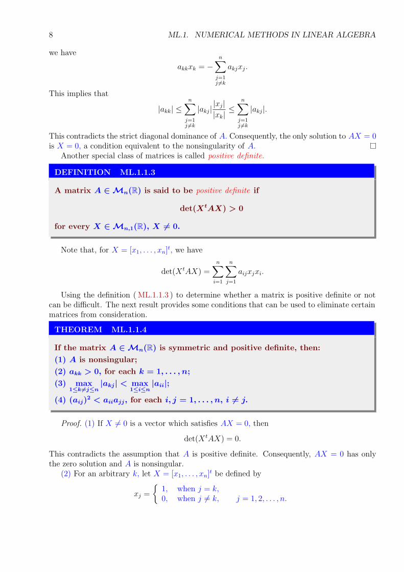
8 ML.1. NUMERICAL METHODS IN LINEAR ALGEBRA
we have
akkxk = −n∑
j=1j 6=k
akjxj.
This implies that
|akk| ≤n∑
j=1j 6=k
|akj||xj||xk|≤
n∑
j=1j 6=k
|akj |.
This contradicts the strict diagonal dominance of A. Consequently, the only solution to AX = 0is X = 0, a condition equivalent to the nonsingularity of A.
Another special class of matrices is called positive definite.
DEFINITION ML.1.1.3
A matrix A ∈ Mn(R) is said to be positive definite if
det(XtAX) > 0
for every X ∈ Mn,1(R), X 6= 0.
Note that, for X = [x1, . . . , xn]t, we have
det(X tAX) =n∑
i=1
n∑
j=1
aijxjxi.
Using the definition ( ML.1.1.3 ) to determine whether a matrix is positive definite or notcan be difficult. The next result provides some conditions that can be used to eliminate certainmatrices from consideration.
THEOREM ML.1.1.4
If the matrix A ∈ Mn(R) is symmetric and positive definite, then:
(1) A is nonsingular;
(2) akk > 0, for each k = 1, . . . , n;
(3) max1≤k 6=j≤n
|akj| < max1≤i≤n
|aii|;
(4) (aij)2 < aiiajj, for each i, j = 1, . . . , n, i 6= j.
Proof. (1) If X 6= 0 is a vector which satisfies AX = 0, then
det(X tAX) = 0.
This contradicts the assumption that A is positive definite. Consequently, AX = 0 has onlythe zero solution and A is nonsingular.
(2) For an arbitrary k, let X = [x1, . . . , xn]t be defined by
xj =
{1, when j = k,0, when j 6= k, j = 1, 2, . . . , n.
ML.1.2. NORMS OF VECTORS AND MATRICES 9
Since X 6= 0, akk = det(X tAX) > 0.(3) For k 6= j define X = [x1, . . . , xn]t by
xi =
0, when i 6= j and i 6= k,−1, when i = j,
1, when i = k.
Since X 6= 0, ajj + akk − ajk − akj = det(X tAX) > 0. But At = A, so ajk = akj and2akj < ajj + akk.
Define Z = [z1, . . . , zn]t where
zi =
{0, when i 6= j and i 6= k,1, when i = j or i = k,
Then det(ZtAZ) > 0, so −2akj < akk + ajj . We obtain
|akj | <akk + ajj
2≤ max
1≤i≤n|aii|.
Hencemax
1≤k 6=j≤n|akj| < max
1≤i≤n|aii|.
(4) For i 6= j, define X = [x1, . . . , xn]t by
xk =
0, when k 6= j and k 6= i,α, when k = i,1, when k = j.
where α represents an arbitrary real number. Since X 6= 0,
0 < det(X tAX) = aiiα2 + 2aijα + ajj .
As a quadratic polynomial in α with no real roots, the discriminant must be negative. Thus
4(a2ij − aiiajj) < 0
anda2
ij < aiiajj .
ML.1.2 Norms of Vectors and Matrices
DEFINITION ML.1.2.1
A vector norm is a function ‖∙‖ : Mn,1(R) → R satisfying the following conditions:
(1) ‖X‖ ≥ 0 for all X ∈ Mn,1(R),
(2) ‖X‖ = 0 if and only if X = 0,
(3) ‖αX‖ = |α|‖X‖ for all α ∈ R and X ∈ Mn,1(R),
(4) ‖X + Y ‖ ≤ ‖X‖ + ‖Y ‖ for all X, Y ∈ Mn,1(R).
10 ML.1. NUMERICAL METHODS IN LINEAR ALGEBRA
The most common vector norms for n-dimensional column vectors with real number coeffi-cients, X = [x1, . . . , xn]t ∈Mn,1(R), are defined by:
‖X‖1 =n∑
i=1
|xi|,
‖X‖2 =
√√√√
n∑
i=1
x2i ,
‖X‖∞ = max1≤i≤n
|xi|,
The norm of a vector gives a measure for the distance between an arbitrary vector and thezero vector. The distance between two vectors can be defined as the norm of the difference ofthe vectors. The concept of distance in Mn,1(R) is also used to define the limit of a sequenceof vectors.
DEFINITION ML.1.2.2
A sequence (X(k))∞k=1 of vectors in Mn,1(R) is said to be convergent to a vectorX ∈ Mn,1(R), with respect to the norm ‖ ∙ ‖, if
limk→∞
‖X(k) − X‖ = 0.
The notion of vector norm will be extended for matrices.
DEFINITION ML.1.2.3
A matrix norm on the set Mn(R) is a function ‖ ∙ ‖ : Mn(R) → R satisfying theconditions:
(1) ‖A‖ ≥ 0,
(2) ‖A‖ = 0 if and only if A = 0,
(3) ‖αA‖ = |α|‖A‖,
(4) ‖A + B‖ ≤ ‖A‖ + ‖B‖,
(5) ‖AB‖ ≤ ‖A‖ ∙ ‖B‖,for all matrices A, B ∈ Mn(R) and any real number α.
It is not difficult to show that if ‖ ∙ ‖ is a vector norm on Mn,1(R), then
‖A‖ := max‖X‖=1
‖AX‖
is a matrix norm called the natural norm or the induced matrix norm associated with thevector norm. In this text, all matrix norms will be assumed to be natural matrix norms unlessspecified otherwise.
ML.1.2. NORMS OF VECTORS AND MATRICES 11
The ‖ ∙ ‖∞ norm of a matrix has an interesting representation with respect to the entries ofthe matrix.
THEOREM ML.1.2.4
If A = [aij] ∈ Mn(R), then
‖A‖∞ = max1≤i≤n
n∑
j=1
|aij|.
Proof. Let X ∈Mn,1(R) be an arbitrary column vector with
1 = ‖X‖∞ = max1≤i≤n
|xi|.
We have:
‖AX‖∞ = max1≤i≤n
|(AX)i|
= max1≤i≤n
∣∣∣∣∣
n∑
j=1
aijxj
∣∣∣∣∣≤ max
1≤i≤n
n∑
j=1
|aij| ∙ max1≤j≤n
|xj|
= max1≤i≤n
n∑
j=1
|aij| ∙ 1.
Consequently,
‖A‖∞ = max‖X‖=1
‖AX‖∞ ≤ max1≤i≤n
n∑
j=1
|aij| (~)
However, if p is an integer such that
n∑
j=1
|apj | = max1≤i≤n
n∑
j=1
|aij |
and X is chosen with
xj =
{1, when apj ≥ 0,−1, when apj < 0,
then ‖X‖∞ = 1 and apjxj = |apj | for j = 1, . . . , n. So
‖AX‖∞ = max1≤i≤n
∣∣∣∣∣
n∑
j=1
aijxj
∣∣∣∣∣
≥
∣∣∣∣∣
n∑
j=1
apjxj
∣∣∣∣∣=
n∑
j=1
|apj | = max1≤i≤n
n∑
j=1
|aij|,
which, together with inequality (~), gives
‖A‖∞ = max1≤i≤n
n∑
j=1
|aij |.
12 ML.1. NUMERICAL METHODS IN LINEAR ALGEBRA
Similarly, we can prove that
‖A‖1 = max1≤j≤n
n∑
i=1
|aij|.
An alternative method for finding ‖A‖2 will be presented in the next section (see Theo-rem ( ML.1.11.5 )).
DEFINITION ML.1.2.5
The Frobenius norm (which is not a natural norm) is defined, for a matrix A =[aij] ∈ Mn(R), by
‖A‖F =
√√√√
n∑
i=1
n∑
j=1
|aij|2.
One can easily prove that, for any matrix A,
‖A‖2 ≤ ‖A‖F ≤√
n ‖A‖2.
Another matrix norm can be defined by
‖A‖ =n∑
i=1
n∑
j=1
|aij |.
Note that the function defined by
f(A) = max1≤i,j≤n
|aij |
is not a norm.
ML.1.2. NORMS OF VECTORS AND MATRICES 13
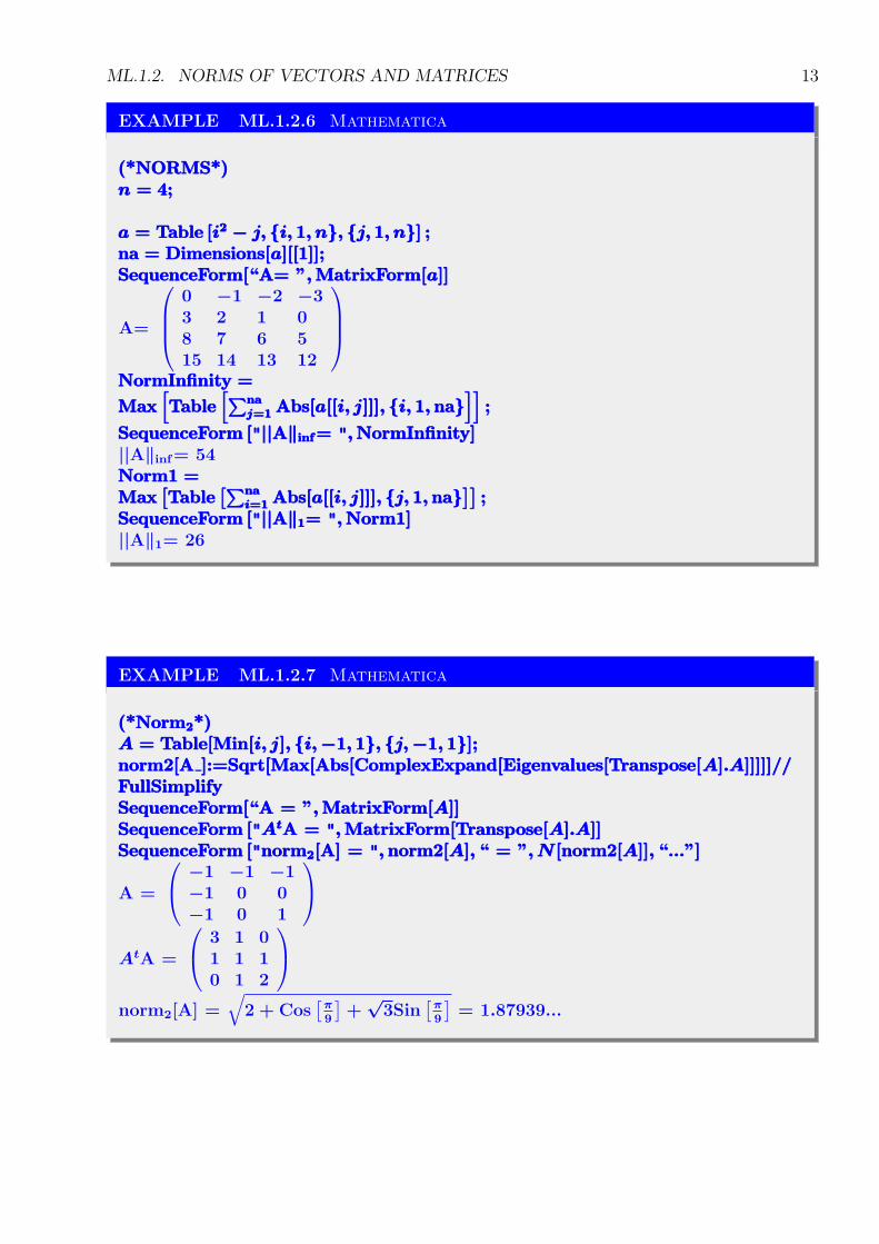
EXAMPLE ML.1.2.6 Mathematica
(*NORMS*)(*NORMS*)(*NORMS*)n = 4;n = 4;n = 4;
a = Table [i2 − j, {i, 1, n}, {j, 1, n}] ;a = Table [i2 − j, {i, 1, n}, {j, 1, n}] ;a = Table [i2 − j, {i, 1, n}, {j, 1, n}] ;na = Dimensions[a][[1]];na = Dimensions[a][[1]];na = Dimensions[a][[1]];SequenceForm[“A= ”, MatrixForm[a]]SequenceForm[“A= ”, MatrixForm[a]]SequenceForm[“A= ”, MatrixForm[a]]
A=
0 −1 −2 −33 2 1 08 7 6 515 14 13 12
NormInfinity =NormInfinity =NormInfinity =
Max[Table
[∑naj=1 Abs[a[[i, j]]], {i, 1, na}
]];Max
[Table
[∑naj=1 Abs[a[[i, j]]], {i, 1, na}
]];Max
[Table
[∑naj=1 Abs[a[[i, j]]], {i, 1, na}
]];
SequenceForm ["||A‖inf= ", NormInfinity]SequenceForm ["||A‖inf= ", NormInfinity]SequenceForm ["||A‖inf= ", NormInfinity]||A‖inf= 54Norm1 =Norm1 =Norm1 =Max
[Table
[∑nai=1 Abs[a[[i, j]]], {j, 1, na}
]];Max
[Table
[∑nai=1 Abs[a[[i, j]]], {j, 1, na}
]];Max
[Table
[∑nai=1 Abs[a[[i, j]]], {j, 1, na}
]];
SequenceForm ["||A‖1= ", Norm1]SequenceForm ["||A‖1= ", Norm1]SequenceForm ["||A‖1= ", Norm1]||A‖1= 26
EXAMPLE ML.1.2.7 Mathematica
(*Norm2*)(*Norm2*)(*Norm2*)A = Table[Min[i, j], {i, −1, 1}, {j, −1, 1}];A = Table[Min[i, j], {i, −1, 1}, {j, −1, 1}];A = Table[Min[i, j], {i, −1, 1}, {j, −1, 1}];norm2[A ]:=Sqrt[Max[Abs[ComplexExpand[Eigenvalues[Transpose[A].A]]]]]//norm2[A ]:=Sqrt[Max[Abs[ComplexExpand[Eigenvalues[Transpose[A].A]]]]]//norm2[A ]:=Sqrt[Max[Abs[ComplexExpand[Eigenvalues[Transpose[A].A]]]]]//FullSimplifyFullSimplifyFullSimplifySequenceForm[“A = ”, MatrixForm[A]]SequenceForm[“A = ”, MatrixForm[A]]SequenceForm[“A = ”, MatrixForm[A]]SequenceForm ["AtA = ", MatrixForm[Transpose[A].A]]SequenceForm ["AtA = ", MatrixForm[Transpose[A].A]]SequenceForm ["AtA = ", MatrixForm[Transpose[A].A]]SequenceForm ["norm2[A] = ", norm2[A], “ = ”, N [norm2[A]], “...”]SequenceForm ["norm2[A] = ", norm2[A], “ = ”, N [norm2[A]], “...”]SequenceForm ["norm2[A] = ", norm2[A], “ = ”, N [norm2[A]], “...”]
A =
−1 −1 −1−1 0 0−1 0 1
AtA =
3 1 01 1 10 1 2
norm2[A] =√
2 + Cos[π9
]+
√3Sin
[π9
]= 1.87939...
14 ML.1. NUMERICAL METHODS IN LINEAR ALGEBRA
ML.1.3 Error Estimation
Consider the linear system
AX = B,
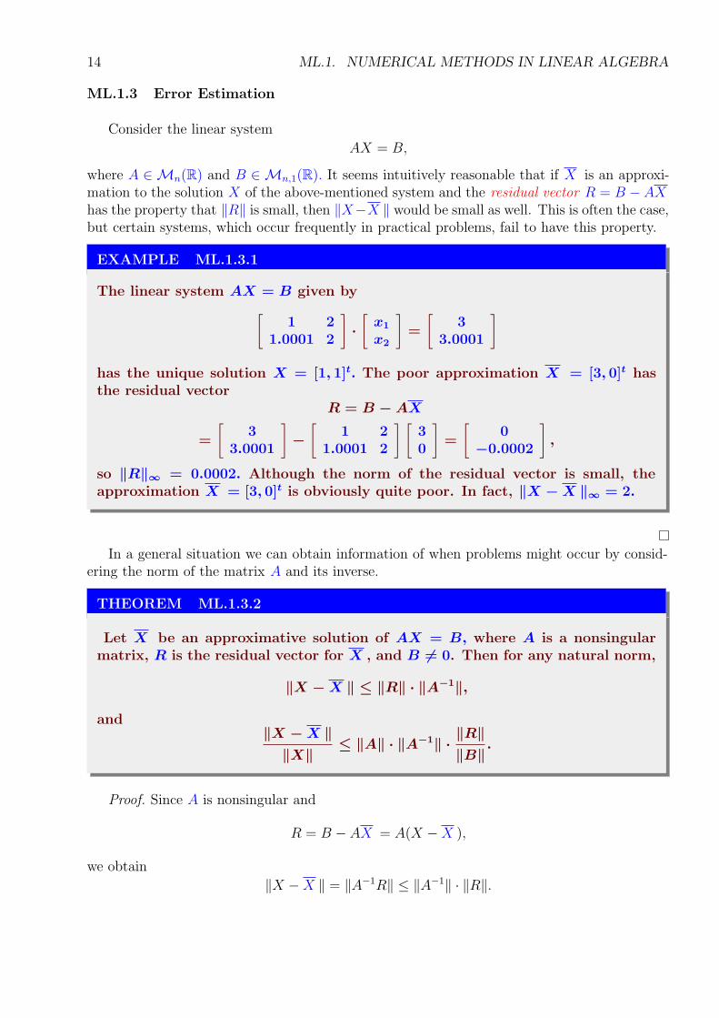
where A ∈ Mn(R) and B ∈ Mn,1(R). It seems intuitively reasonable that if X is an approxi-mation to the solution X of the above-mentioned system and the residual vector R = B − AXhas the property that ‖R‖ is small, then ‖X−X ‖ would be small as well. This is often the case,but certain systems, which occur frequently in practical problems, fail to have this property.
EXAMPLE ML.1.3.1
The linear system AX = B given by
[1 2
1.0001 2
]
∙
[x1
x2
]
=
[3
3.0001
]
has the unique solution X = [1, 1]t. The poor approximation X = [3, 0]t hasthe residual vector
R = B − AX
=
[3
3.0001
]
−
[1 2
1.0001 2
] [30
]
=
[0
−0.0002
]
,
so ‖R‖∞ = 0.0002. Although the norm of the residual vector is small, theapproximation X = [3, 0]t is obviously quite poor. In fact, ‖X − X ‖∞ = 2.
In a general situation we can obtain information of when problems might occur by consid-ering the norm of the matrix A and its inverse.
THEOREM ML.1.3.2
Let X be an approximative solution of AX = B, where A is a nonsingularmatrix, R is the residual vector for X , and B 6= 0. Then for any natural norm,
‖X − X ‖ ≤ ‖R‖ ∙ ‖A−1‖,
and‖X − X ‖
‖X‖≤ ‖A‖ ∙ ‖A−1‖ ∙
‖R‖
‖B‖.
Proof. Since A is nonsingular and
R = B − AX = A(X −X ),
we obtain
‖X −X ‖ = ‖A−1R‖ ≤ ‖A−1‖ ∙ ‖R‖.
ML.1.3. ERROR ESTIMATION 15
Moreover, since B = AX, we have
‖B‖ ≤ ‖A‖ ∙ ‖X‖,
and‖X −X ‖‖X‖
≤‖A‖ ∙ ‖A−1‖‖B‖
∙ ‖R‖.
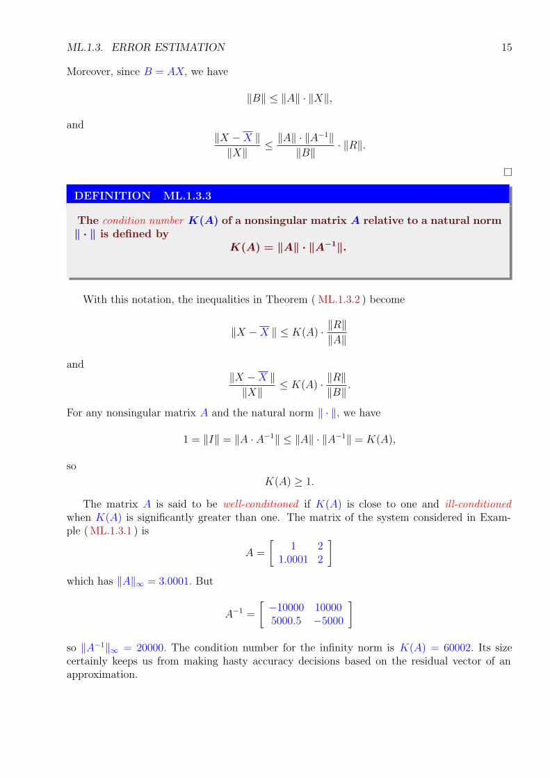
DEFINITION ML.1.3.3
The condition number K(A) of a nonsingular matrix A relative to a natural norm‖ ∙ ‖ is defined by
K(A) = ‖A‖ ∙ ‖A−1‖.
With this notation, the inequalities in Theorem ( ML.1.3.2 ) become
‖X −X ‖ ≤ K(A) ∙‖R‖‖A‖
and‖X −X ‖‖X‖
≤ K(A) ∙‖R‖‖B‖
.
For any nonsingular matrix A and the natural norm ‖ ∙ ‖, we have
1 = ‖I‖ = ‖A ∙ A−1‖ ≤ ‖A‖ ∙ ‖A−1‖ = K(A),
so
K(A) ≥ 1.
The matrix A is said to be well-conditioned if K(A) is close to one and ill-conditionedwhen K(A) is significantly greater than one. The matrix of the system considered in Exam-ple ( ML.1.3.1 ) is
A =
[1 2
1.0001 2
]
which has ‖A‖∞ = 3.0001. But
A−1 =
[−10000 100005000.5 −5000
]
so ‖A−1‖∞ = 20000. The condition number for the infinity norm is K(A) = 60002. Its sizecertainly keeps us from making hasty accuracy decisions based on the residual vector of anapproximation.
16 ML.1. NUMERICAL METHODS IN LINEAR ALGEBRA
ML.1.4 Matrix Equations. Pivoting Elimination
Matrix equations are associated with many problems arising in engineering and science, aswell as with applications of mathematics to social sciences. For solving a matrix equation, thepartial pivoting elimination is about as efficient as any other method.
Pivoting is a process of interchanging rows (partial pivoting) or rows and columns (fullpivoting), so as to put a particularly desirable element in the diagonal position from which thepivot is about to be selected.
Let us recall the principal row elementary operations used to transform a matrix equationto a more convenient one with the same solution:
1. Multiply the row i by a nonzero constant λ. This operation is denoted by
ri ← λ ri.
2. Add the row j multiplied by a constant λ to the row i. This operation is denoted by
ri ← ri + λ rj .
3. Interchange rows i and j. This operation is denoted by
ri rj .
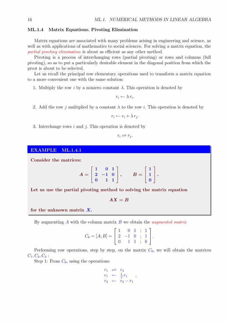
EXAMPLE ML.1.4.1
Consider the matrices:
A =
1 0 12 −1 00 1 1
, B =
110
.
Let us use the partial pivoting method to solving the matrix equation
AX = B
for the unknown matrix X.
By augmenting A with the column matrix B we obtain the augmented matrix
C0 = [A; B] =
1 0 1 ; 12 −1 0 ; 10 1 1 ; 0
.
Performing row operations, step by step, on the matrix C0, we will obtain the matricesC1, C2, C3 :
Step 1: From C0, using the operations:
r1 r2
r1 ← 12r1
r2 ← r2 − r1
,
ML.1.4. MATRIX EQUATIONS. PIVOTING ELIMINATION 17
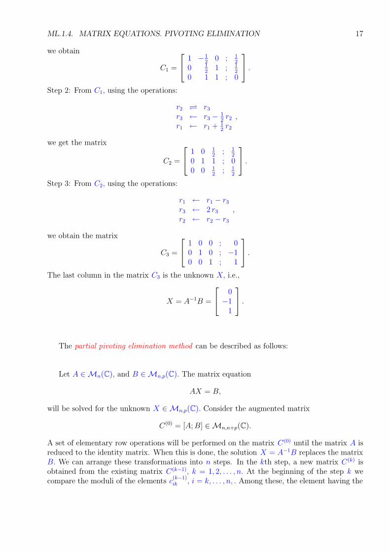
we obtain
C1 =
1 −1
20 ; 1
2
0 12
1 ; 12
0 1 1 ; 0
.
Step 2: From C1, using the operations:
r2 r3
r3 ← r3 − 12r2
r1 ← r1 + 12r2
,
we get the matrix
C2 =
1 0 1
2; 1
2
0 1 1 ; 00 0 1
2; 1
2
.
Step 3: From C2, using the operations:
r1 ← r1 − r3
r3 ← 2 r3
r2 ← r2 − r3
,
we obtain the matrix
C3 =
1 0 0 ; 00 1 0 ; −10 0 1 ; 1
.
The last column in the matrix C3 is the unknown X, i.e.,
X = A−1B =
0−1
1
.
The partial pivoting elimination method can be described as follows:
Let A ∈Mn(C), and B ∈Mn,p(C). The matrix equation
AX = B,
will be solved for the unknown X ∈Mn,p(C). Consider the augmented matrix
C(0) = [A; B] ∈Mn,n+p(C).
A set of elementary row operations will be performed on the matrix C(0) until the matrix A isreduced to the identity matrix. When this is done, the solution X = A−1B replaces the matrixB. We can arrange these transformations into n steps. In the kth step, a new matrix C(k) isobtained from the existing matrix C(k−1), k = 1, 2, . . . , n. At the beginning of the step k wecompare the moduli of the elements c
(k−1)ik , i = k, . . . , n, . Among these, the element having the
18 ML.1. NUMERICAL METHODS IN LINEAR ALGEBRA
largest modulus, is called pivot element. Then, the row containing the pivot element and thekth row are interchanged. If, after last interchange, the modulus of the pivot element c
(k−1)kk
is less than a given value ε, then the matrix A is considered to be singular and the procedurestops.
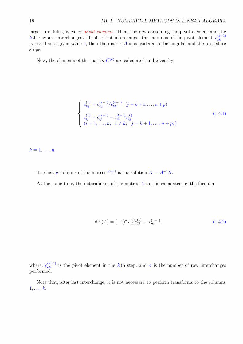
Now, the elements of the matrix C(k) are calculated and given by:
c(k)kj = c
(k−1)kj /c
(k−1)kk (j = k + 1, . . . , n + p)
c(k)ij = c
(k−1)ij − c
(k−1)ik c
(k)kj
(i = 1, . . . , n; i 6= k; j = k + 1, . . . , n + p; )
(1.4.1)
k = 1, . . . , n.
The last p columns of the matrix C(n) is the solution X = A−1B.
At the same time, the determinant of the matrix A can be calculated by the formula
det(A) = (−1)σ c(0)11 c
(1)22 ∙ ∙ ∙ c
(n−1)nn , (1.4.2)
where, c(k−1)kk is the pivot element in the k th step, and σ is the number of row interchanges
performed.
Note that, after last interchange, it is not necessary to perform transforms to the columns1, . . . , k.
ML.1.4. MATRIX EQUATIONS. PIVOTING ELIMINATION 19
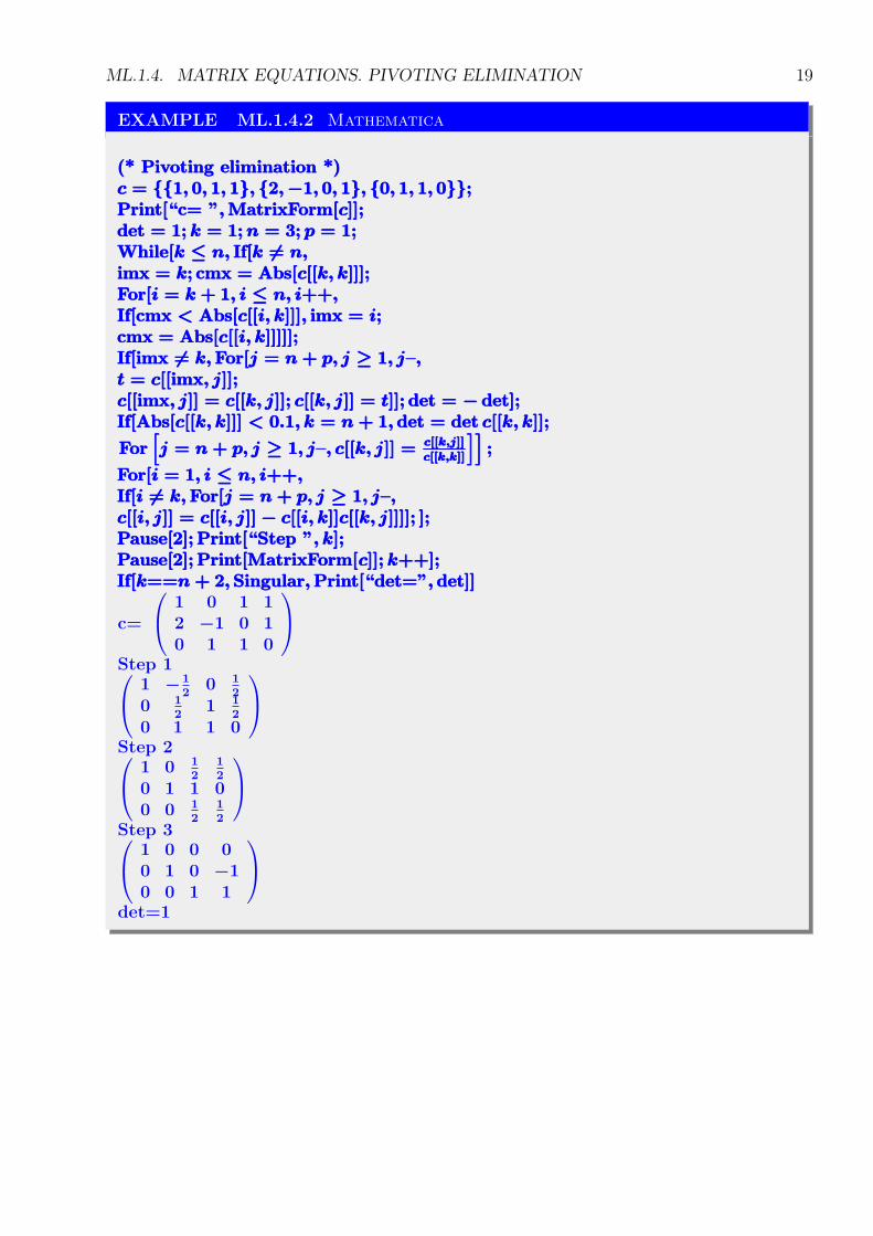
EXAMPLE ML.1.4.2 Mathematica
(* Pivoting elimination *)(* Pivoting elimination *)(* Pivoting elimination *)c = {{1, 0, 1, 1}, {2, −1, 0, 1}, {0, 1, 1, 0}};c = {{1, 0, 1, 1}, {2, −1, 0, 1}, {0, 1, 1, 0}};c = {{1, 0, 1, 1}, {2, −1, 0, 1}, {0, 1, 1, 0}};Print[“c= ”, MatrixForm[c]];Print[“c= ”, MatrixForm[c]];Print[“c= ”, MatrixForm[c]];det = 1; k = 1; n = 3; p = 1;det = 1; k = 1; n = 3; p = 1;det = 1; k = 1; n = 3; p = 1;While[k ≤ n, If[k 6= n,While[k ≤ n, If[k 6= n,While[k ≤ n, If[k 6= n,imx = k; cmx = Abs[c[[k, k]]];imx = k; cmx = Abs[c[[k, k]]];imx = k; cmx = Abs[c[[k, k]]];For[i = k + 1, i ≤ n, i++,For[i = k + 1, i ≤ n, i++,For[i = k + 1, i ≤ n, i++,If[cmx < Abs[c[[i, k]]], imx = i;If[cmx < Abs[c[[i, k]]], imx = i;If[cmx < Abs[c[[i, k]]], imx = i;cmx = Abs[c[[i, k]]]]];cmx = Abs[c[[i, k]]]]];cmx = Abs[c[[i, k]]]]];If[imx 6= k, For[j = n + p, j ≥ 1, j–,If[imx 6= k, For[j = n + p, j ≥ 1, j–,If[imx 6= k, For[j = n + p, j ≥ 1, j–,t = c[[imx, j]];t = c[[imx, j]];t = c[[imx, j]];c[[imx, j]] = c[[k, j]]; c[[k, j]] = t]]; det = − det];c[[imx, j]] = c[[k, j]]; c[[k, j]] = t]]; det = − det];c[[imx, j]] = c[[k, j]]; c[[k, j]] = t]]; det = − det];If[Abs[c[[k, k]]] < 0.1, k = n + 1, det = det c[[k, k]];If[Abs[c[[k, k]]] < 0.1, k = n + 1, det = det c[[k, k]];If[Abs[c[[k, k]]] < 0.1, k = n + 1, det = det c[[k, k]];
For[j = n + p, j ≥ 1, j–, c[[k, j]] = c[[k,j]]
c[[k,k]]
]];For
[j = n + p, j ≥ 1, j–, c[[k, j]] = c[[k,j]]
c[[k,k]]
]];For
[j = n + p, j ≥ 1, j–, c[[k, j]] = c[[k,j]]
c[[k,k]]
]];
For[i = 1, i ≤ n, i++,For[i = 1, i ≤ n, i++,For[i = 1, i ≤ n, i++,If[i 6= k, For[j = n + p, j ≥ 1, j–,If[i 6= k, For[j = n + p, j ≥ 1, j–,If[i 6= k, For[j = n + p, j ≥ 1, j–,c[[i, j]] = c[[i, j]] − c[[i, k]]c[[k, j]]]]; ];c[[i, j]] = c[[i, j]] − c[[i, k]]c[[k, j]]]]; ];c[[i, j]] = c[[i, j]] − c[[i, k]]c[[k, j]]]]; ];Pause[2]; Print[“Step ”, k];Pause[2]; Print[“Step ”, k];Pause[2]; Print[“Step ”, k];Pause[2]; Print[MatrixForm[c]]; k++];Pause[2]; Print[MatrixForm[c]]; k++];Pause[2]; Print[MatrixForm[c]]; k++];If[k==n + 2, Singular, Print[“det=”, det]]If[k==n + 2, Singular, Print[“det=”, det]]If[k==n + 2, Singular, Print[“det=”, det]]
c=
1 0 1 12 −1 0 10 1 1 0
Step 1
1 −1
20 1
2
0 12
1 12
0 1 1 0
Step 2
1 0 1
212
0 1 1 00 0 1
212
Step 3
1 0 0 00 1 0 −10 0 1 1
det=1
20 ML.1. NUMERICAL METHODS IN LINEAR ALGEBRA
REMARK ML.1.4.3
• If p = n and B is the identity matrix, then the solution of the equationAX = B is A−1.• If p = 1 we obtain the Gauss-Jordan method for solving linear system of equa-tions.• If A is a strictly diagonally dominant matrix, the Gaussian elimination canbe performed on any linear system AX = B without row interchange, and thecomputations are stable with respect to the growth of round-off errors [BF93,p 372].
ML.1.5 Improved Solutions of Matrix Equations
Obviously it is not easy to obtain greater precision for the solution of a matrix equationthan the precision of the computer’s floating-point word. Unfortunately, for large sets of lin-ear equations, it is not always easy to obtain precision equal to, or even comparable to thecomputer’s limits.
In the direct methods of solution, roundoff errors are accumulated and they magnify to theextend when the matrix is close to singular.
Suppose that the matrix X is the exact solution of the equation
AX = B.
We don’t, however, know X. We only know some slightly wrong solution say X . Substitutingthis into AX = B we obtain
B = AX .
In order to find a correction matrix E(X) we solve the equation
A ∙ E(X) = B − B = AX − AX ,
where the right-hand side B − B is known. We obtain a slightly wrong correction E(X) . So,
X + E(X)
is an improved solution. An extra benefit occurs if we repeat the previous steps.
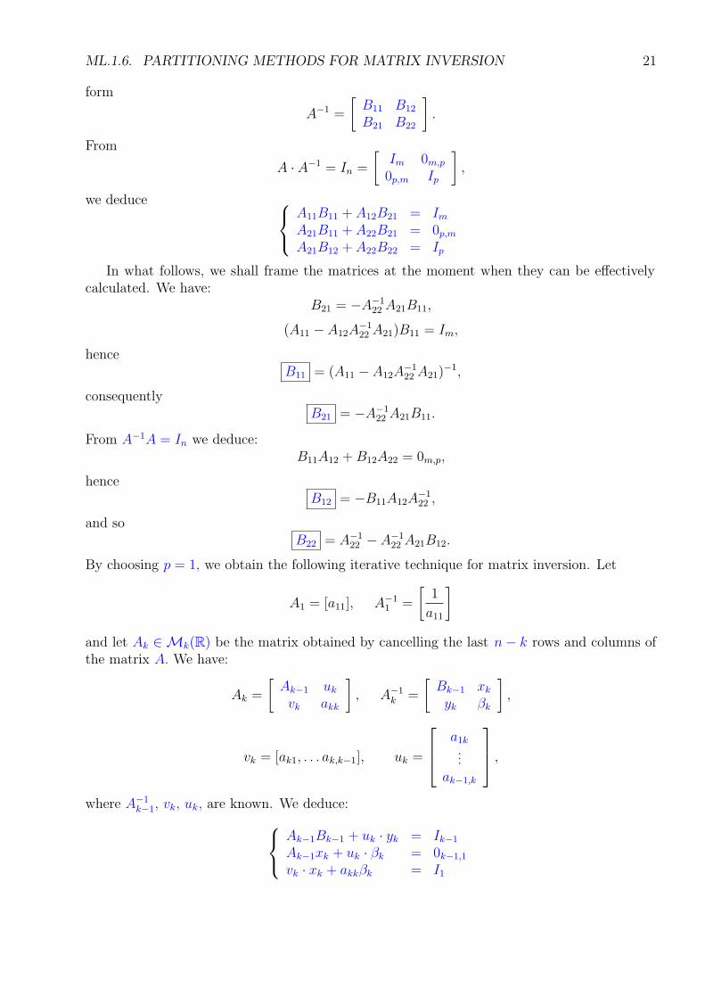
ML.1.6 Partitioning Methods for Matrix Inversion
Let A ∈Mn(R) be a nonsingular matrix. Consider the partition
A =
[A11 A12
A21 A22
]
where A11 ∈Mm(R), A12 ∈Mm,p(R), A21 ∈Mp,m(R), and A22 ∈Mp(R), such that m+p = n.In order to compute the inverse of the matrix A, we shall try to find the matrix A−1 into the
ML.1.6. PARTITIONING METHODS FOR MATRIX INVERSION 21
form
A−1 =
[B11 B12
B21 B22
]
.
From
A ∙ A−1 = In =
[Im 0m,p
0p,m Ip
]
,
we deduce
A11B11 + A12B21 = Im
A21B11 + A22B21 = 0p,m
A21B12 + A22B22 = Ip
In what follows, we shall frame the matrices at the moment when they can be effectivelycalculated. We have:
B21 = −A−122 A21B11,
(A11 − A12A−122 A21)B11 = Im,
henceB11 = (A11 − A12A
−122 A21)
−1,
consequentlyB21 = −A−1
22 A21B11.
From A−1A = In we deduce:B11A12 + B12A22 = 0m,p,
henceB12 = −B11A12A
−122 ,
and soB22 = A−1
22 − A−122 A21B12.
By choosing p = 1, we obtain the following iterative technique for matrix inversion. Let
A1 = [a11], A−11 =
[1
a11
]
and let Ak ∈ Mk(R) be the matrix obtained by cancelling the last n− k rows and columns ofthe matrix A. We have:
Ak =
[Ak−1 uk
vk akk
]
, A−1k =
[Bk−1 xk
yk βk
]
,
vk = [ak1, . . . ak,k−1], uk =
a1k...
ak−1,k
,
where A−1k−1, vk, uk, are known. We deduce:
Ak−1Bk−1 + uk ∙ yk = Ik−1
Ak−1xk + uk ∙ βk = 0k−1,1
vk ∙ xk + akkβk = I1
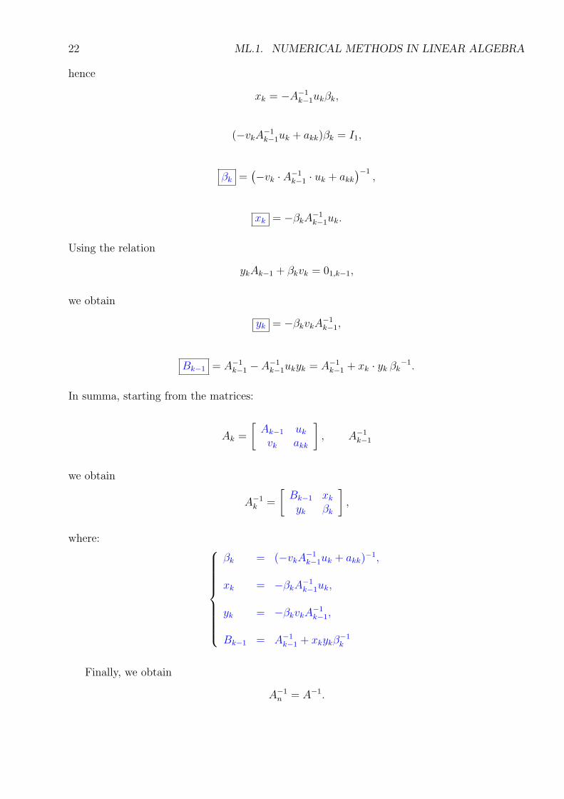
22 ML.1. NUMERICAL METHODS IN LINEAR ALGEBRA
hence
xk = −A−1k−1ukβk,
(−vkA−1k−1uk + akk)βk = I1,
βk =(−vk ∙ A
−1k−1 ∙ uk + akk
)−1,
xk = −βkA−1k−1uk.
Using the relation
ykAk−1 + βkvk = 01,k−1,
we obtain
yk = −βkvkA−1k−1,
Bk−1 = A−1k−1 − A−1
k−1ukyk = A−1k−1 + xk ∙ yk βk
−1.
In summa, starting from the matrices:
Ak =
[Ak−1 uk
vk akk
]
, A−1k−1
we obtain
A−1k =
[Bk−1 xk
yk βk
]
,
where:
βk = (−vkA−1k−1uk + akk)
−1,
xk = −βkA−1k−1uk,
yk = −βkvkA−1k−1,
Bk−1 = A−1k−1 + xkykβ
−1k
Finally, we obtain
A−1n = A−1.
ML.1.7. LU FACTORIZATION 23
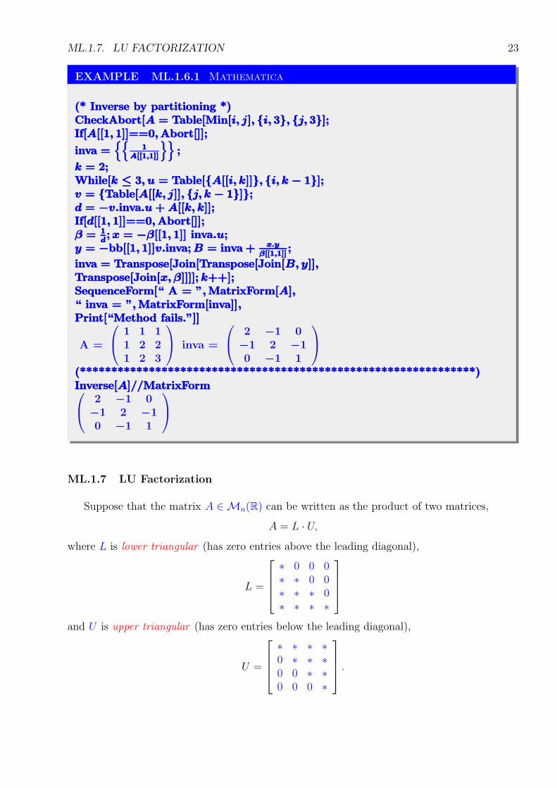
EXAMPLE ML.1.6.1 Mathematica
(* Inverse by partitioning *)(* Inverse by partitioning *)(* Inverse by partitioning *)CheckAbort[A = Table[Min[i, j], {i, 3}, {j, 3}];CheckAbort[A = Table[Min[i, j], {i, 3}, {j, 3}];CheckAbort[A = Table[Min[i, j], {i, 3}, {j, 3}];If[A[[1, 1]]==0, Abort[]];If[A[[1, 1]]==0, Abort[]];If[A[[1, 1]]==0, Abort[]];
inva ={{
1A[[1,1]]
}};inva =
{{1
A[[1,1]]
}};inva =
{{1
A[[1,1]]
}};
k = 2;k = 2;k = 2;While[k ≤ 3, u = Table[{A[[i, k]]}, {i, k − 1}];While[k ≤ 3, u = Table[{A[[i, k]]}, {i, k − 1}];While[k ≤ 3, u = Table[{A[[i, k]]}, {i, k − 1}];v = {Table[A[[k, j]], {j, k − 1}]};v = {Table[A[[k, j]], {j, k − 1}]};v = {Table[A[[k, j]], {j, k − 1}]};d = −v.inva.u + A[[k, k]];d = −v.inva.u + A[[k, k]];d = −v.inva.u + A[[k, k]];If[d[[1, 1]]==0, Abort[]];If[d[[1, 1]]==0, Abort[]];If[d[[1, 1]]==0, Abort[]];β = 1
d; x = −β[[1, 1]] inva.u;β = 1d; x = −β[[1, 1]] inva.u;β = 1d; x = −β[[1, 1]] inva.u;
y = −bb[[1, 1]]v.inva; B = inva + x.y
β[[1,1]];y = −bb[[1, 1]]v.inva; B = inva + x.y
β[[1,1]];y = −bb[[1, 1]]v.inva; B = inva + x.y
β[[1,1]];
inva = Transpose[Join[Transpose[Join[B, y]],inva = Transpose[Join[Transpose[Join[B, y]],inva = Transpose[Join[Transpose[Join[B, y]],Transpose[Join[x, β]]]]; k++];Transpose[Join[x, β]]]]; k++];Transpose[Join[x, β]]]]; k++];SequenceForm[“ A = ”, MatrixForm[A],SequenceForm[“ A = ”, MatrixForm[A],SequenceForm[“ A = ”, MatrixForm[A],“ inva = ”, MatrixForm[inva]],“ inva = ”, MatrixForm[inva]],“ inva = ”, MatrixForm[inva]],Print[“Method fails.”]]Print[“Method fails.”]]Print[“Method fails.”]]
A =
1 1 11 2 21 2 3
inva =
2 −1 0
−1 2 −10 −1 1
(***************************************************************)(***************************************************************)(***************************************************************)Inverse[A]//MatrixFormInverse[A]//MatrixFormInverse[A]//MatrixForm
2 −1 0
−1 2 −10 −1 1
ML.1.7 LU Factorization
Suppose that the matrix A ∈Mn(R) can be written as the product of two matrices,
A = L ∙ U,
where L is lower triangular (has zero entries above the leading diagonal),
L =
∗ 0 0 0∗ ∗ 0 0∗ ∗ ∗ 0∗ ∗ ∗ ∗
and U is upper triangular (has zero entries below the leading diagonal),
U =
∗ ∗ ∗ ∗0 ∗ ∗ ∗0 0 ∗ ∗0 0 0 ∗
.
24 ML.1. NUMERICAL METHODS IN LINEAR ALGEBRA
The matrix A has an LU factorization or LU decomposition.
The LU factorization of a matrix A can be used to solve the linear system of equations
AX = B.
Using the LU factorization we can solve the system by using a two-step process. We write thesystem into the form
L(UX) = B.
First solve the system
LY = B
for Y. Since L is triangular, determining Y from this equation requires only O(n2) operations.Next, the triangular system
UX = Y
requires an additional O(n2) operations to determine the solution X. It is to be noted that onlyO(n2) number of operations is required to solve the system AX = B compared with O(n3)needed by the Gaussian elimination. Determining the specific matrices L and U requires O(n3)operations, but, once the factorization is determined, any system involving the matrix A canbe solved in the simplified manner.
ML.1.7. LU FACTORIZATION 25
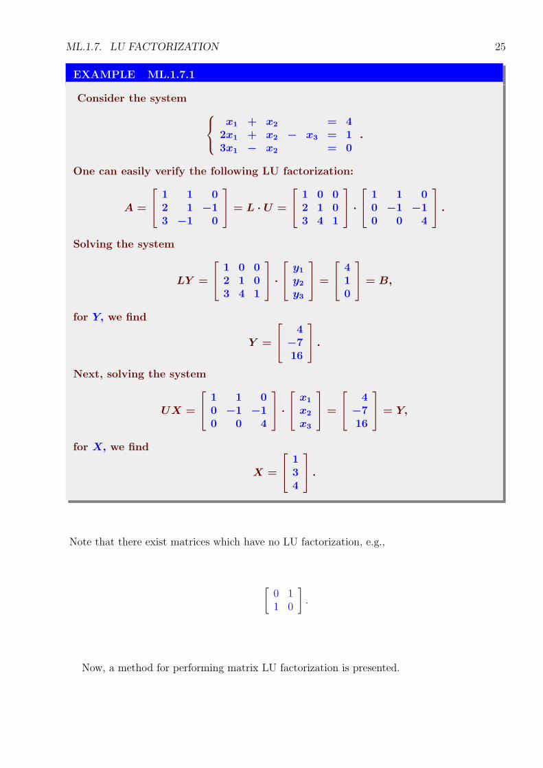
EXAMPLE ML.1.7.1
Consider the system
x1 + x2 = 42x1 + x2 − x3 = 13x1 − x2 = 0
.
One can easily verify the following LU factorization:
A =
1 1 02 1 −13 −1 0
= L ∙ U =
1 0 02 1 03 4 1
∙
1 1 00 −1 −10 0 4
.
Solving the system
LY =
1 0 02 1 03 4 1
∙
y1
y2
y3
=
410
= B,
for Y, we find
Y =
4
−716
.
Next, solving the system
UX =
1 1 00 −1 −10 0 4
∙
x1
x2
x3
=
4
−716
= Y,
for X, we find
X =
134
.
Note that there exist matrices which have no LU factorization, e.g.,
[0 11 0
]
.
Now, a method for performing matrix LU factorization is presented.
26 ML.1. NUMERICAL METHODS IN LINEAR ALGEBRA
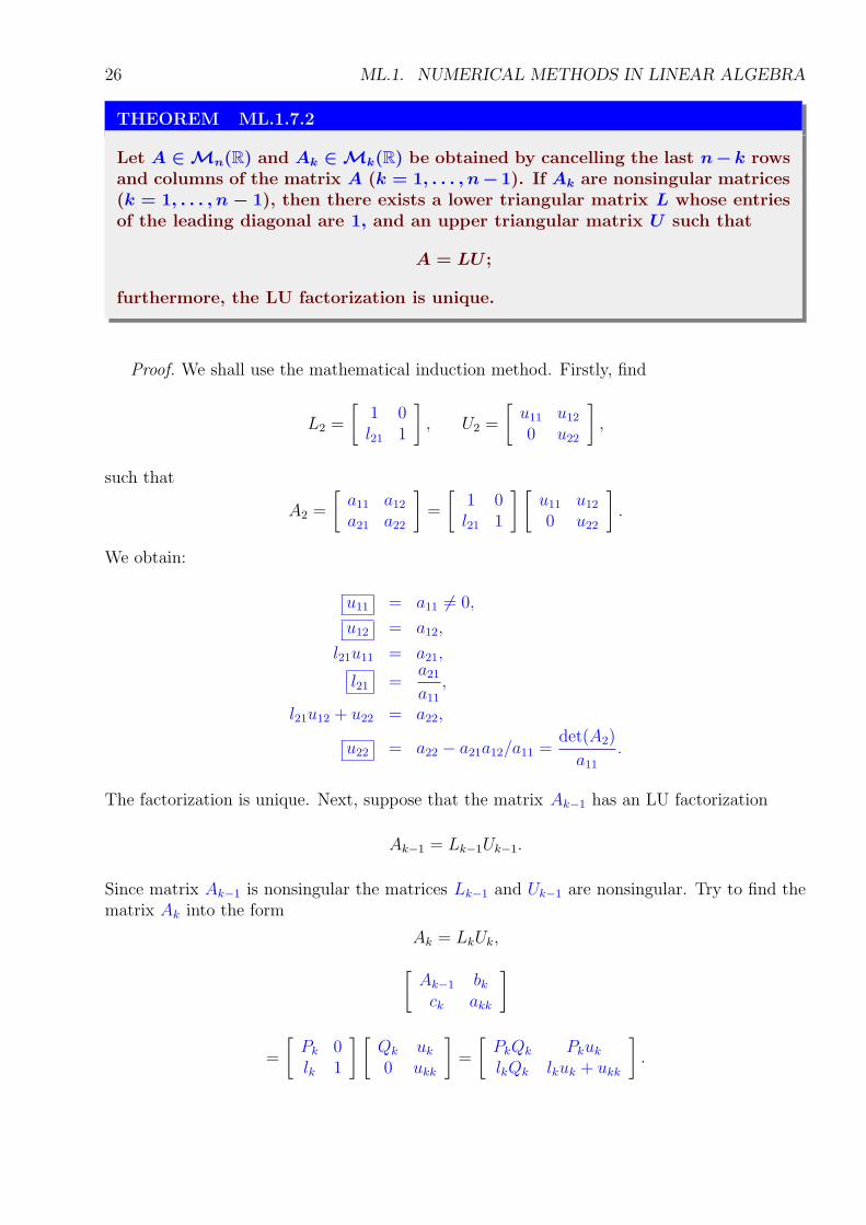
THEOREM ML.1.7.2
Let A ∈ Mn(R) and Ak ∈ Mk(R) be obtained by cancelling the last n − k rowsand columns of the matrix A (k = 1, . . . , n − 1). If Ak are nonsingular matrices(k = 1, . . . , n − 1), then there exists a lower triangular matrix L whose entriesof the leading diagonal are 1, and an upper triangular matrix U such that
A = LU ;
furthermore, the LU factorization is unique.
Proof. We shall use the mathematical induction method. Firstly, find
L2 =
[1 0l21 1
]
, U2 =
[u11 u12
0 u22
]
,
such that
A2 =
[a11 a12
a21 a22
]
=
[1 0l21 1
] [u11 u12
0 u22
]
.
We obtain:
u11 = a11 6= 0,
u12 = a12,
l21u11 = a21,
l21 =a21
a11
,
l21u12 + u22 = a22,
u22 = a22 − a21a12/a11 =det(A2)
a11
.
The factorization is unique. Next, suppose that the matrix Ak−1 has an LU factorization
Ak−1 = Lk−1Uk−1.
Since matrix Ak−1 is nonsingular the matrices Lk−1 and Uk−1 are nonsingular. Try to find thematrix Ak into the form
Ak = LkUk,
[Ak−1 bk
ck akk
]
=
[Pk 0lk 1
] [Qk uk
0 ukk
]
=
[PkQk Pkuk
lkQk lkuk + ukk
]
.
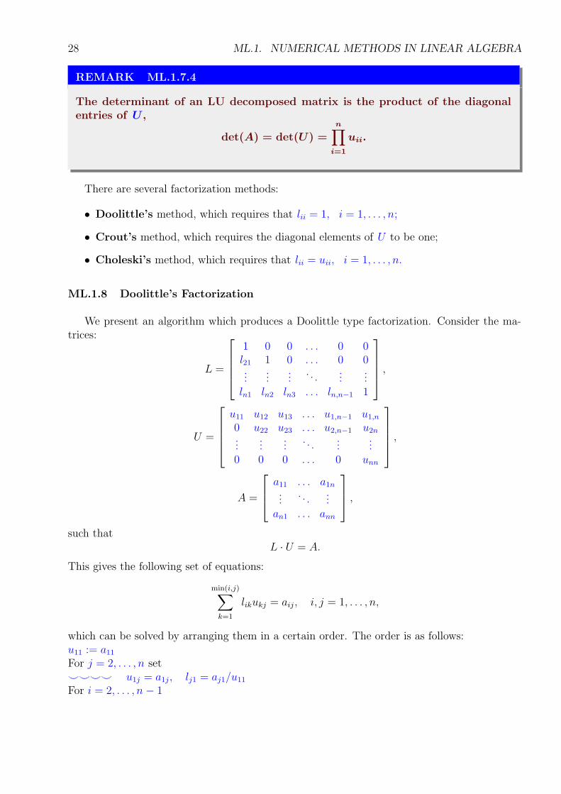
ML.1.7. LU FACTORIZATION 27
From Ak−1 = PkQk, and using the uniqueness property of the factorization, we obtain:
Pk = Lk−1,
Qk = Uk−1,
Lk−1uk = bk,
uk = L−1k−1bk,
lkUk−1 = ck
lk = ckU−1k−1
lkuk + ukk = akk,
ukk = akk − lkuk.
For k = n the existence and the uniqueness of the LU factorization are proved. Following theproof, we obtain a recurrent method for finding the matrices L and U.
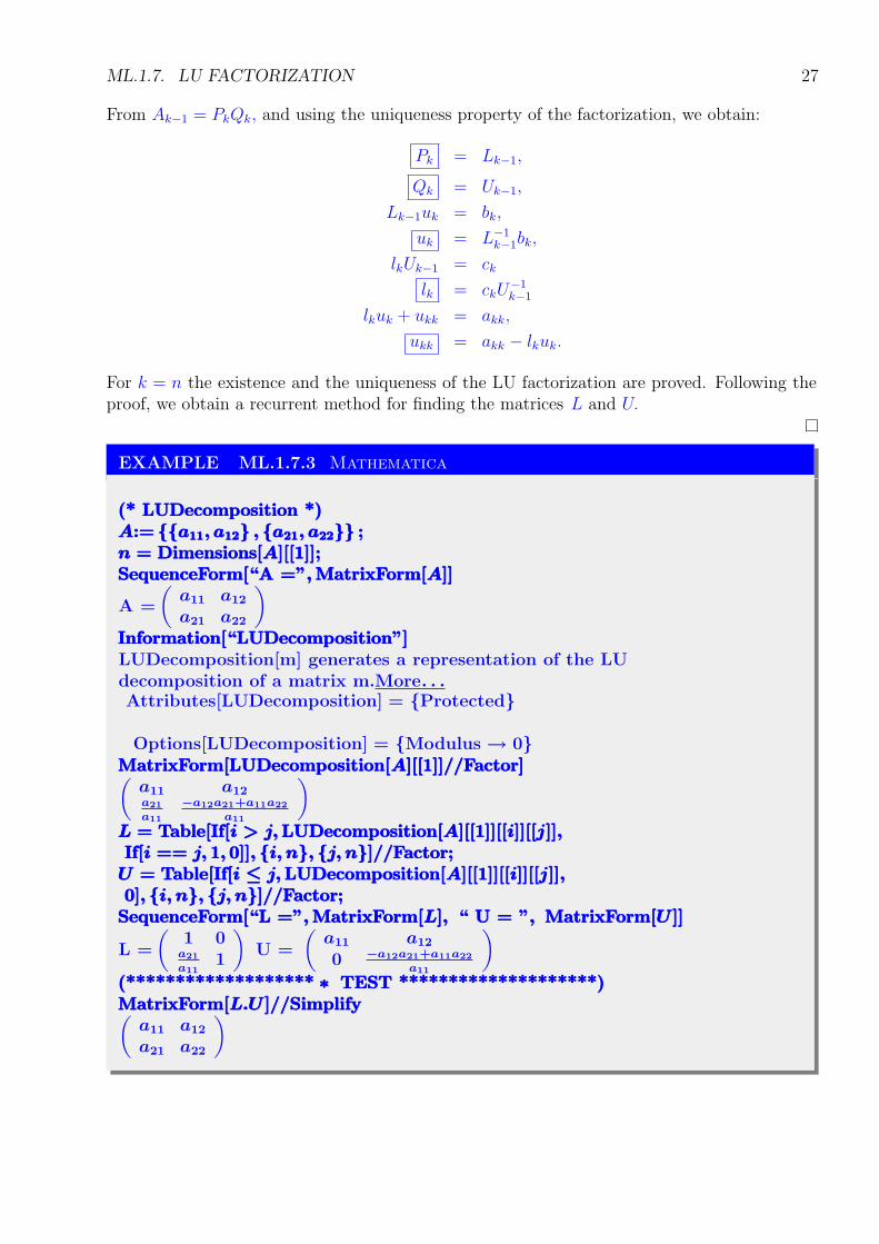
EXAMPLE ML.1.7.3 Mathematica
(* LUDecomposition *)(* LUDecomposition *)(* LUDecomposition *)A:= {{a11, a12} , {a21, a22}} ;A:= {{a11, a12} , {a21, a22}} ;A:= {{a11, a12} , {a21, a22}} ;n = Dimensions[A][[1]];n = Dimensions[A][[1]];n = Dimensions[A][[1]];SequenceForm[“A =”, MatrixForm[A]]SequenceForm[“A =”, MatrixForm[A]]SequenceForm[“A =”, MatrixForm[A]]
A =
(a11 a12
a21 a22
)
Information[“LUDecomposition”]Information[“LUDecomposition”]Information[“LUDecomposition”]LUDecomposition[m] generates a representation of the LUdecomposition of a matrix m.More. . .Attributes[LUDecomposition] = {Protected}
Options[LUDecomposition] = {Modulus → 0}MatrixForm[LUDecomposition[A][[1]]//Factor]MatrixForm[LUDecomposition[A][[1]]//Factor]MatrixForm[LUDecomposition[A][[1]]//Factor](
a11 a12a21a11
−a12a21+a11a22a11
)
L = Table[If[i > j, LUDecomposition[A][[1]][[i]][[j]],L = Table[If[i > j, LUDecomposition[A][[1]][[i]][[j]],L = Table[If[i > j, LUDecomposition[A][[1]][[i]][[j]],If[i == j, 1, 0]], {i, n}, {j, n}]//Factor;If[i == j, 1, 0]], {i, n}, {j, n}]//Factor;If[i == j, 1, 0]], {i, n}, {j, n}]//Factor;
U = Table[If[i ≤ j, LUDecomposition[A][[1]][[i]][[j]],U = Table[If[i ≤ j, LUDecomposition[A][[1]][[i]][[j]],U = Table[If[i ≤ j, LUDecomposition[A][[1]][[i]][[j]],0], {i, n}, {j, n}]//Factor;0], {i, n}, {j, n}]//Factor;0], {i, n}, {j, n}]//Factor;
SequenceForm[“L =”, MatrixForm[L], “ U = ”, MatrixForm[U ]]SequenceForm[“L =”, MatrixForm[L], “ U = ”, MatrixForm[U ]]SequenceForm[“L =”, MatrixForm[L], “ U = ”, MatrixForm[U ]]
L =
(1 0a21a11
1
)
U =
(a11 a12
0 −a12a21+a11a22a11
)
(******************* ∗ TEST ********************)(******************* ∗ TEST ********************)(******************* ∗ TEST ********************)MatrixForm[L.U ]//SimplifyMatrixForm[L.U ]//SimplifyMatrixForm[L.U ]//Simplify(
a11 a12
a21 a22
)
28 ML.1. NUMERICAL METHODS IN LINEAR ALGEBRA
REMARK ML.1.7.4
The determinant of an LU decomposed matrix is the product of the diagonalentries of U ,
det(A) = det(U) =n∏
i=1
uii.
There are several factorization methods:
• Doolittle’s method, which requires that lii = 1, i = 1, . . . , n;
• Crout’s method, which requires the diagonal elements of U to be one;
• Choleski’s method, which requires that lii = uii, i = 1, . . . , n.
ML.1.8 Doolittle’s Factorization
We present an algorithm which produces a Doolittle type factorization. Consider the ma-trices:
L =
1 0 0 . . . 0 0l21 1 0 . . . 0 0...
......
. . ....
...ln1 ln2 ln3 . . . ln,n−1 1
,
U =
u11 u12 u13 . . . u1,n−1 u1,n
0 u22 u23 . . . u2,n−1 u2n...
......
. . ....
...0 0 0 . . . 0 unn
,
A =
a11 . . . a1n...
. . ....
an1 . . . ann
,
such thatL ∙ U = A.
This gives the following set of equations:
min(i,j)∑
k=1
likukj = aij , i, j = 1, . . . , n,
which can be solved by arranging them in a certain order. The order is as follows:u11 := a11
For j = 2, . . . , n set^^^^ u1j = a1j , lj1 = aj1/u11
For i = 2, . . . , n − 1
ML.1.8. DOOLITTLE’S FACTORIZATION 29
^^^^ uii = aii −i−1∑
k=1
likuki
^^^^ For j = i + 1, . . . , n
^^^^^^^^ uij = aij −i−1∑
k=1
likukj
^^^^^^^^ lji =
(
aji −i−1∑
k=1
ljkuki
)
/uii
unn = ann −n−1∑
k=1
lnkukn
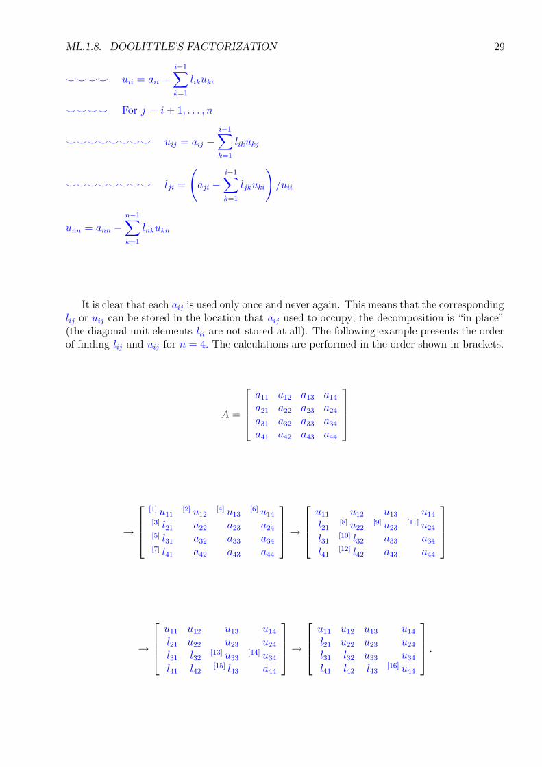
It is clear that each aij is used only once and never again. This means that the correspondinglij or uij can be stored in the location that aij used to occupy; the decomposition is “in place”(the diagonal unit elements lii are not stored at all). The following example presents the orderof finding lij and uij for n = 4. The calculations are performed in the order shown in brackets.
A =
a11 a12 a13 a14
a21 a22 a23 a24
a31 a32 a33 a34
a41 a42 a43 a44
→
[1] u11[2] u12
[4] u13[6] u14
[3] l21 a22 a23 a24[5] l31 a32 a33 a34[7] l41 a42 a43 a44
→
u11 u12 u13 u14
l21[8] u22
[9] u23[11] u24
l31[10] l32 a33 a34
l41[12] l42 a43 a44
→
u11 u12 u13 u14
l21 u22 u23 u24
l31 l32[13] u33
[14] u34
l41 l42[15] l43 a44
→
u11 u12 u13 u14
l21 u22 u23 u24
l31 l32 u33 u34
l41 l42 l43[16] u44
.
30 ML.1. NUMERICAL METHODS IN LINEAR ALGEBRA
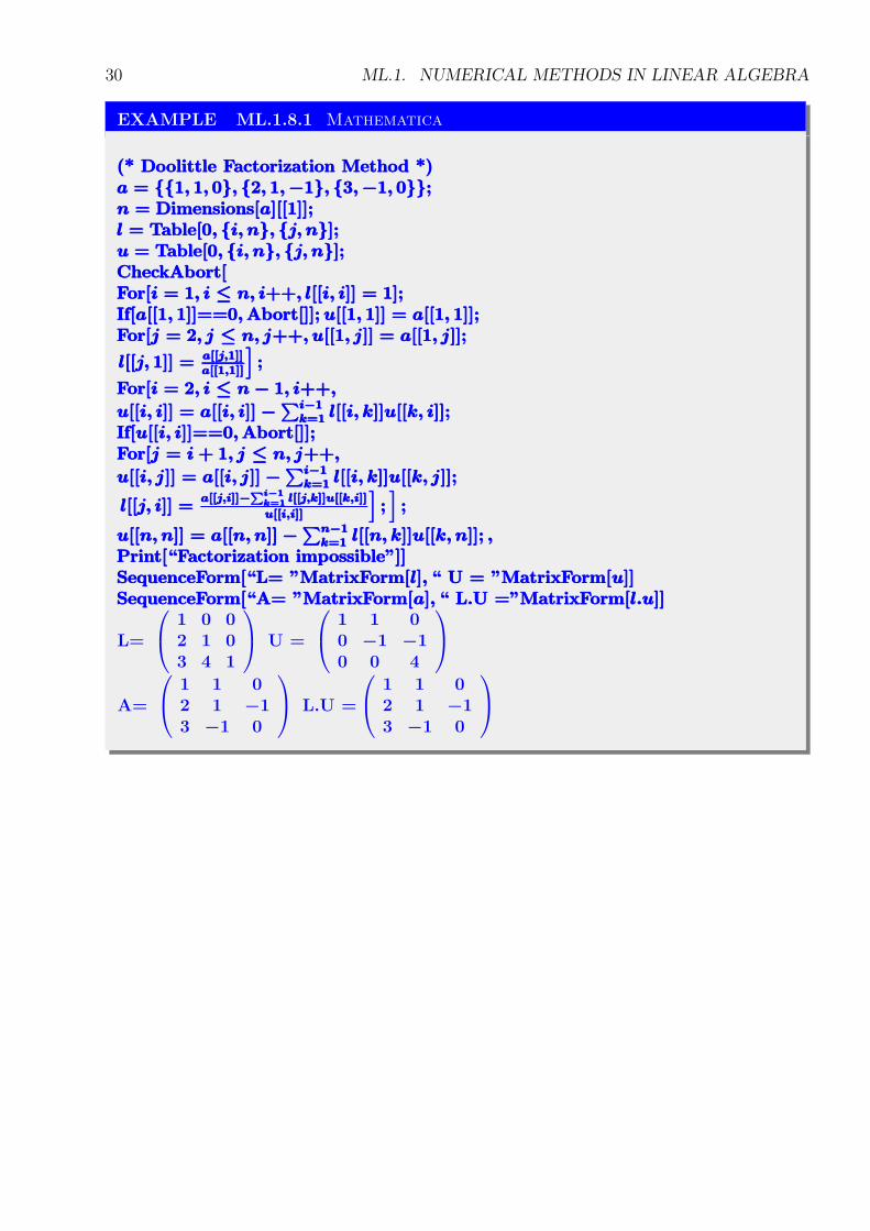
EXAMPLE ML.1.8.1 Mathematica
(* Doolittle Factorization Method *)(* Doolittle Factorization Method *)(* Doolittle Factorization Method *)a = {{1, 1, 0}, {2, 1, −1}, {3, −1, 0}};a = {{1, 1, 0}, {2, 1, −1}, {3, −1, 0}};a = {{1, 1, 0}, {2, 1, −1}, {3, −1, 0}};n = Dimensions[a][[1]];n = Dimensions[a][[1]];n = Dimensions[a][[1]];l = Table[0, {i, n}, {j, n}];l = Table[0, {i, n}, {j, n}];l = Table[0, {i, n}, {j, n}];u = Table[0, {i, n}, {j, n}];u = Table[0, {i, n}, {j, n}];u = Table[0, {i, n}, {j, n}];CheckAbort[CheckAbort[CheckAbort[For[i = 1, i ≤ n, i++, l[[i, i]] = 1];For[i = 1, i ≤ n, i++, l[[i, i]] = 1];For[i = 1, i ≤ n, i++, l[[i, i]] = 1];If[a[[1, 1]]==0, Abort[]]; u[[1, 1]] = a[[1, 1]];If[a[[1, 1]]==0, Abort[]]; u[[1, 1]] = a[[1, 1]];If[a[[1, 1]]==0, Abort[]]; u[[1, 1]] = a[[1, 1]];For[j = 2, j ≤ n, j++, u[[1, j]] = a[[1, j]];For[j = 2, j ≤ n, j++, u[[1, j]] = a[[1, j]];For[j = 2, j ≤ n, j++, u[[1, j]] = a[[1, j]];
l[[j, 1]] = a[[j,1]]
a[[1,1]]
];l[[j, 1]] = a[[j,1]]
a[[1,1]]
];l[[j, 1]] = a[[j,1]]
a[[1,1]]
];
For[i = 2, i ≤ n − 1, i++,For[i = 2, i ≤ n − 1, i++,For[i = 2, i ≤ n − 1, i++,
u[[i, i]] = a[[i, i]] −∑i−1k=1 l[[i, k]]u[[k, i]];u[[i, i]] = a[[i, i]] −
∑i−1k=1 l[[i, k]]u[[k, i]];u[[i, i]] = a[[i, i]] −
∑i−1k=1 l[[i, k]]u[[k, i]];
If[u[[i, i]]==0, Abort[]];If[u[[i, i]]==0, Abort[]];If[u[[i, i]]==0, Abort[]];For[j = i + 1, j ≤ n, j++,For[j = i + 1, j ≤ n, j++,For[j = i + 1, j ≤ n, j++,
u[[i, j]] = a[[i, j]] −∑i−1k=1 l[[i, k]]u[[k, j]];u[[i, j]] = a[[i, j]] −
∑i−1k=1 l[[i, k]]u[[k, j]];u[[i, j]] = a[[i, j]] −
∑i−1k=1 l[[i, k]]u[[k, j]];
l[[j, i]] =a[[j,i]]−
∑i−1k=1 l[[j,k]]u[[k,i]]
u[[i,i]]
];];l[[j, i]] =
a[[j,i]]−∑i−1k=1 l[[j,k]]u[[k,i]]
u[[i,i]]
];];l[[j, i]] =
a[[j,i]]−∑i−1k=1 l[[j,k]]u[[k,i]]
u[[i,i]]
];];
u[[n, n]] = a[[n, n]] −∑n−1k=1 l[[n, k]]u[[k, n]]; ,u[[n, n]] = a[[n, n]] −
∑n−1k=1 l[[n, k]]u[[k, n]]; ,u[[n, n]] = a[[n, n]] −
∑n−1k=1 l[[n, k]]u[[k, n]]; ,
Print[“Factorization impossible”]]Print[“Factorization impossible”]]Print[“Factorization impossible”]]SequenceForm[“L= ”MatrixForm[l], “ U = ”MatrixForm[u]]SequenceForm[“L= ”MatrixForm[l], “ U = ”MatrixForm[u]]SequenceForm[“L= ”MatrixForm[l], “ U = ”MatrixForm[u]]SequenceForm[“A= ”MatrixForm[a], “ L.U =”MatrixForm[l.u]]SequenceForm[“A= ”MatrixForm[a], “ L.U =”MatrixForm[l.u]]SequenceForm[“A= ”MatrixForm[a], “ L.U =”MatrixForm[l.u]]
L=
1 0 02 1 03 4 1
U =
1 1 00 −1 −10 0 4
A=
1 1 02 1 −13 −1 0
L.U =
1 1 02 1 −13 −1 0
ML.1.9. CHOLESKI’S FACTORIZATION METHOD 31
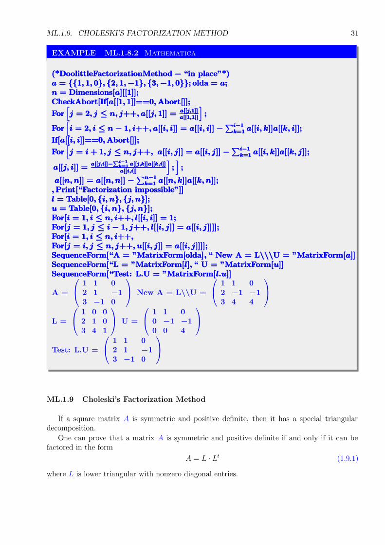
EXAMPLE ML.1.8.2 Mathematica
(*DoolittleFactorizationMethod − “in place”*)(*DoolittleFactorizationMethod − “in place”*)(*DoolittleFactorizationMethod − “in place”*)a = {{1, 1, 0}, {2, 1, −1}, {3, −1, 0}}; olda = a;a = {{1, 1, 0}, {2, 1, −1}, {3, −1, 0}}; olda = a;a = {{1, 1, 0}, {2, 1, −1}, {3, −1, 0}}; olda = a;n = Dimensions[a][[1]];n = Dimensions[a][[1]];n = Dimensions[a][[1]];CheckAbort[If[a[[1, 1]]==0, Abort[]];CheckAbort[If[a[[1, 1]]==0, Abort[]];CheckAbort[If[a[[1, 1]]==0, Abort[]];
For[j = 2, j ≤ n, j++, a[[j, 1]] = a[[j,1]]
a[[1,1]]
];For
[j = 2, j ≤ n, j++, a[[j, 1]] = a[[j,1]]
a[[1,1]]
];For
[j = 2, j ≤ n, j++, a[[j, 1]] = a[[j,1]]
a[[1,1]]
];
For[i = 2, i ≤ n − 1, i++, a[[i, i]] = a[[i, i]] −
∑i−1k=1 a[[i, k]]a[[k, i]];For
[i = 2, i ≤ n − 1, i++, a[[i, i]] = a[[i, i]] −
∑i−1k=1 a[[i, k]]a[[k, i]];For
[i = 2, i ≤ n − 1, i++, a[[i, i]] = a[[i, i]] −
∑i−1k=1 a[[i, k]]a[[k, i]];
If[a[[i, i]]==0, Abort[]];If[a[[i, i]]==0, Abort[]];If[a[[i, i]]==0, Abort[]];
For[j = i + 1, j ≤ n, j++, a[[i, j]] = a[[i, j]] −
∑i−1k=1 a[[i, k]]a[[k, j]];For
[j = i + 1, j ≤ n, j++, a[[i, j]] = a[[i, j]] −
∑i−1k=1 a[[i, k]]a[[k, j]];For
[j = i + 1, j ≤ n, j++, a[[i, j]] = a[[i, j]] −
∑i−1k=1 a[[i, k]]a[[k, j]];
a[[j, i]] =a[[j,i]]−
∑i−1k=1 a[[j,k]]a[[k,i]]
a[[i,i]]
];];a[[j, i]] =
a[[j,i]]−∑i−1k=1 a[[j,k]]a[[k,i]]
a[[i,i]]
];];a[[j, i]] =
a[[j,i]]−∑i−1k=1 a[[j,k]]a[[k,i]]
a[[i,i]]
];];
a[[n, n]] = a[[n, n]] −∑n−1k=1 a[[n, k]]a[[k, n]];a[[n, n]] = a[[n, n]] −
∑n−1k=1 a[[n, k]]a[[k, n]];a[[n, n]] = a[[n, n]] −
∑n−1k=1 a[[n, k]]a[[k, n]];
, Print[“Factorization impossible”]], Print[“Factorization impossible”]], Print[“Factorization impossible”]]l = Table[0, {i, n}, {j, n}];l = Table[0, {i, n}, {j, n}];l = Table[0, {i, n}, {j, n}];u = Table[0, {i, n}, {j, n}];u = Table[0, {i, n}, {j, n}];u = Table[0, {i, n}, {j, n}];For[i = 1, i ≤ n, i++, l[[i, i]] = 1;For[i = 1, i ≤ n, i++, l[[i, i]] = 1;For[i = 1, i ≤ n, i++, l[[i, i]] = 1;For[j = 1, j ≤ i − 1, j++, l[[i, j]] = a[[i, j]]]];For[j = 1, j ≤ i − 1, j++, l[[i, j]] = a[[i, j]]]];For[j = 1, j ≤ i − 1, j++, l[[i, j]] = a[[i, j]]]];For[i = 1, i ≤ n, i++,For[i = 1, i ≤ n, i++,For[i = 1, i ≤ n, i++,For[j = i, j ≤ n, j++, u[[i, j]] = a[[i, j]]]];For[j = i, j ≤ n, j++, u[[i, j]] = a[[i, j]]]];For[j = i, j ≤ n, j++, u[[i, j]] = a[[i, j]]]];SequenceForm[“A = ”MatrixForm[olda], “ New A = L\\\U = ”MatrixForm[a]]SequenceForm[“A = ”MatrixForm[olda], “ New A = L\\\U = ”MatrixForm[a]]SequenceForm[“A = ”MatrixForm[olda], “ New A = L\\\U = ”MatrixForm[a]]SequenceForm[“L = ”MatrixForm[l], “ U = ”MatrixForm[u]]SequenceForm[“L = ”MatrixForm[l], “ U = ”MatrixForm[u]]SequenceForm[“L = ”MatrixForm[l], “ U = ”MatrixForm[u]]SequenceForm[“Test: L.U = ”MatrixForm[l.u]]SequenceForm[“Test: L.U = ”MatrixForm[l.u]]SequenceForm[“Test: L.U = ”MatrixForm[l.u]]
A =
1 1 02 1 −13 −1 0
New A = L\\U =
1 1 02 −1 −13 4 4
L =
1 0 02 1 03 4 1
U =
1 1 00 −1 −10 0 4
Test: L.U =
1 1 02 1 −13 −1 0
ML.1.9 Choleski’s Factorization Method
If a square matrix A is symmetric and positive definite, then it has a special triangulardecomposition.
One can prove that a matrix A is symmetric and positive definite if and only if it can befactored in the form
A = L ∙ Lt (1.9.1)
where L is lower triangular with nonzero diagonal entries.
32 ML.1. NUMERICAL METHODS IN LINEAR ALGEBRA
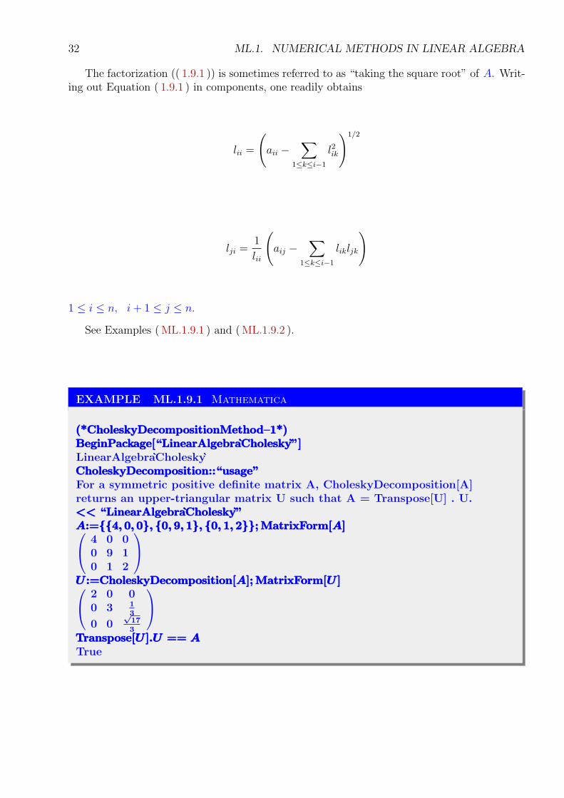
The factorization (( 1.9.1 )) is sometimes referred to as “taking the square root” of A. Writ-ing out Equation ( 1.9.1 ) in components, one readily obtains
lii =
(
aii −∑
1≤k≤i−1
l2ik
)1/2
lji =1
lii
(
aij −∑
1≤k≤i−1
likljk
)
1 ≤ i ≤ n, i + 1 ≤ j ≤ n.
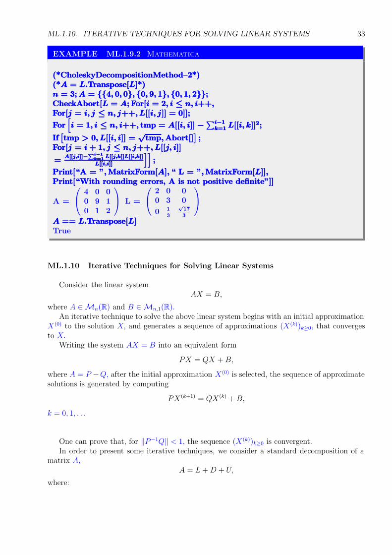
See Examples ( ML.1.9.1 ) and ( ML.1.9.2 ).
EXAMPLE ML.1.9.1 Mathematica
(*CholeskyDecompositionMethod–1*)(*CholeskyDecompositionMethod–1*)(*CholeskyDecompositionMethod–1*)BeginPackage[“LinearAlgebraCholesky”]BeginPackage[“LinearAlgebraCholesky”]BeginPackage[“LinearAlgebraCholesky”]LinearAlgebraCholeskyCholeskyDecomposition::“usage”CholeskyDecomposition::“usage”CholeskyDecomposition::“usage”For a symmetric positive definite matrix A, CholeskyDecomposition[A]returns an upper-triangular matrix U such that A = Transpose[U] . U.<< “LinearAlgebraCholesky”<< “LinearAlgebraCholesky”<< “LinearAlgebraCholesky”A:={{4, 0, 0}, {0, 9, 1}, {0, 1, 2}}; MatrixForm[A]A:={{4, 0, 0}, {0, 9, 1}, {0, 1, 2}}; MatrixForm[A]A:={{4, 0, 0}, {0, 9, 1}, {0, 1, 2}}; MatrixForm[A]
4 0 00 9 10 1 2
U :=CholeskyDecomposition[A]; MatrixForm[U ]U :=CholeskyDecomposition[A]; MatrixForm[U ]U :=CholeskyDecomposition[A]; MatrixForm[U ]
2 0 00 3 1
3
0 0√
173
Transpose[U ].U == ATranspose[U ].U == ATranspose[U ].U == ATrue
ML.1.10. ITERATIVE TECHNIQUES FOR SOLVING LINEAR SYSTEMS 33
EXAMPLE ML.1.9.2 Mathematica
(*CholeskyDecompositionMethod–2*)(*CholeskyDecompositionMethod–2*)(*CholeskyDecompositionMethod–2*)(*A = L.Transpose[L]*)(*A = L.Transpose[L]*)(*A = L.Transpose[L]*)n = 3; A = {{4, 0, 0}, {0, 9, 1}, {0, 1, 2}};n = 3; A = {{4, 0, 0}, {0, 9, 1}, {0, 1, 2}};n = 3; A = {{4, 0, 0}, {0, 9, 1}, {0, 1, 2}};CheckAbort[L = A; For[i = 2, i ≤ n, i++,CheckAbort[L = A; For[i = 2, i ≤ n, i++,CheckAbort[L = A; For[i = 2, i ≤ n, i++,For[j = i, j ≤ n, j++, L[[i, j]] = 0]];For[j = i, j ≤ n, j++, L[[i, j]] = 0]];For[j = i, j ≤ n, j++, L[[i, j]] = 0]];
For[i = 1, i ≤ n, i++, tmp = A[[i, i]] −
∑i−1k=1 L[[i, k]]2;For
[i = 1, i ≤ n, i++, tmp = A[[i, i]] −
∑i−1k=1 L[[i, k]]2;For
[i = 1, i ≤ n, i++, tmp = A[[i, i]] −
∑i−1k=1 L[[i, k]]2;
If[tmp > 0, L[[i, i]] =
√tmp, Abort[]
];If
[tmp > 0, L[[i, i]] =
√tmp, Abort[]
];If
[tmp > 0, L[[i, i]] =
√tmp, Abort[]
];
For[j = i + 1, j ≤ n, j++, L[[j, i]]For[j = i + 1, j ≤ n, j++, L[[j, i]]For[j = i + 1, j ≤ n, j++, L[[j, i]]
=A[[j,i]]−
∑i−1k=1 L[[j,k]]L[[i,k]]
L[[i,i]]
]];=
A[[j,i]]−∑i−1k=1 L[[j,k]]L[[i,k]]
L[[i,i]]
]];=
A[[j,i]]−∑i−1k=1 L[[j,k]]L[[i,k]]
L[[i,i]]
]];
Print[“A = ”, MatrixForm[A], “ L = ”, MatrixForm[L]],Print[“A = ”, MatrixForm[A], “ L = ”, MatrixForm[L]],Print[“A = ”, MatrixForm[A], “ L = ”, MatrixForm[L]],Print[“With rounding errors, A is not positive definite”]]Print[“With rounding errors, A is not positive definite”]]Print[“With rounding errors, A is not positive definite”]]
A =
4 0 00 9 10 1 2
L =
2 0 00 3 0
0 13
√173
A == L.Transpose[L]A == L.Transpose[L]A == L.Transpose[L]True
ML.1.10 Iterative Techniques for Solving Linear Systems
Consider the linear systemAX = B,
where A ∈Mn(R) and B ∈Mn,1(R).An iterative technique to solve the above linear system begins with an initial approximation
X(0) to the solution X, and generates a sequence of approximations (X(k))k≥0, that convergesto X.
Writing the system AX = B into an equivalent form
PX = QX + B,
where A = P −Q, after the initial approximation X(0) is selected, the sequence of approximatesolutions is generated by computing
PX(k+1) = QX(k) + B,
k = 0, 1, . . .
One can prove that, for ‖P−1Q‖ < 1, the sequence (X(k))k≥0 is convergent.In order to present some iterative techniques, we consider a standard decomposition of a
matrix A,A = L + D + U,
where:
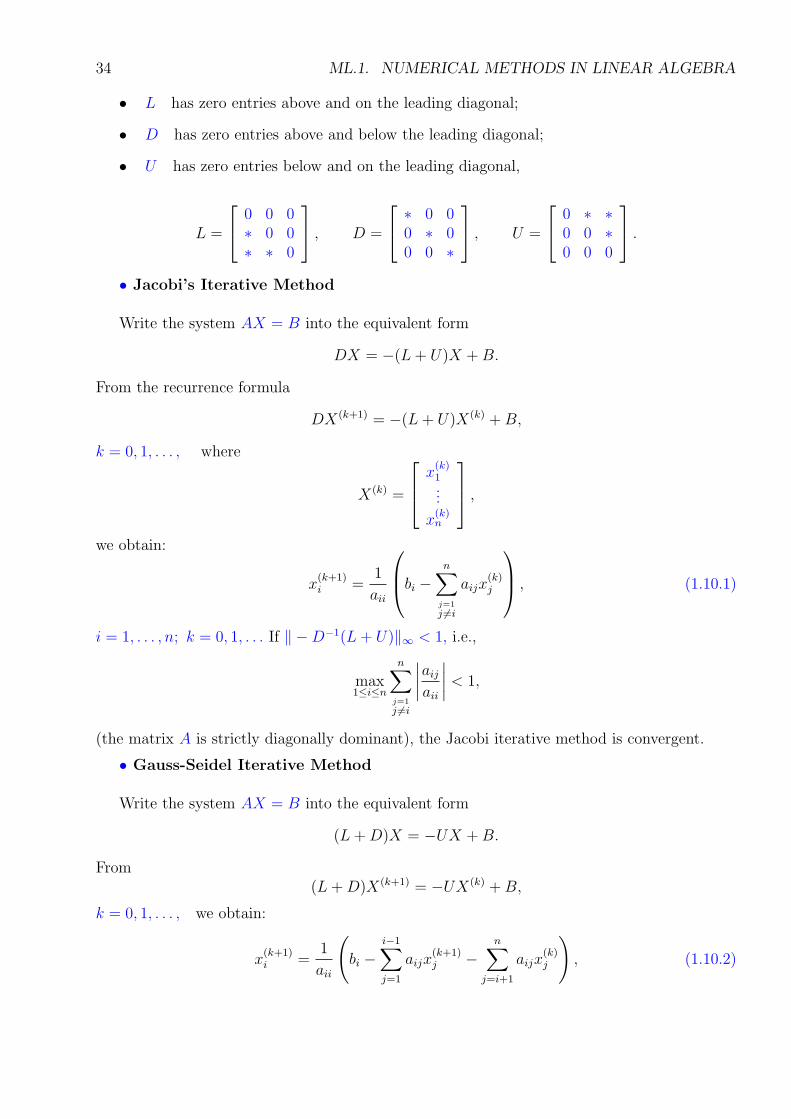
34 ML.1. NUMERICAL METHODS IN LINEAR ALGEBRA
• L has zero entries above and on the leading diagonal;
• D has zero entries above and below the leading diagonal;
• U has zero entries below and on the leading diagonal,
L =
0 0 0∗ 0 0∗ ∗ 0
, D =
∗ 0 00 ∗ 00 0 ∗
, U =
0 ∗ ∗0 0 ∗0 0 0
.
• Jacobi’s Iterative Method
Write the system AX = B into the equivalent form
DX = −(L + U)X + B.
From the recurrence formula
DX(k+1) = −(L + U)X(k) + B,
k = 0, 1, . . . , where
X(k) =
x(k)1...
x(k)n
,
we obtain:
x(k+1)i =
1
aii
bi −
n∑
j=1
j 6=i
aijx(k)j
, (1.10.1)
i = 1, . . . , n; k = 0, 1, . . . If ‖ −D−1(L + U)‖∞ < 1, i.e.,
max1≤i≤n
n∑
j=1
j 6=i
∣∣∣∣aij
aii
∣∣∣∣ < 1,
(the matrix A is strictly diagonally dominant), the Jacobi iterative method is convergent.
• Gauss-Seidel Iterative Method
Write the system AX = B into the equivalent form
(L + D)X = −UX + B.
From(L + D)X(k+1) = −UX(k) + B,
k = 0, 1, . . . , we obtain:
x(k+1)i =
1
aii
(
bi −i−1∑
j=1
aijx(k+1)j −
n∑
j=i+1
aijx(k)j
)
, (1.10.2)
ML.1.10. ITERATIVE TECHNIQUES FOR SOLVING LINEAR SYSTEMS 35
i = 1, . . . , n. If the matrix A is strictly diagonally dominant, then the Gauss-Seidel method isconvergent.
Note that, there exist linear systems for which the Jacobi method is convergent but not theGauss-Seidel method, and vice versa.
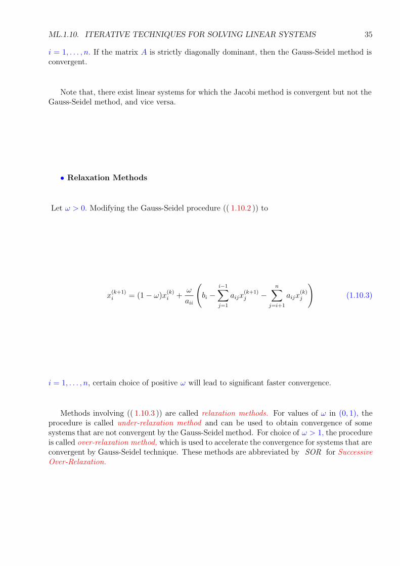
• Relaxation Methods
Let ω > 0. Modifying the Gauss-Seidel procedure (( 1.10.2 )) to
x(k+1)i = (1− ω)x
(k)i +
ω
aii
(
bi −i−1∑
j=1
aijx(k+1)j −
n∑
j=i+1
aijx(k)j
)
(1.10.3)
i = 1, . . . , n, certain choice of positive ω will lead to significant faster convergence.
Methods involving (( 1.10.3 )) are called relaxation methods. For values of ω in (0, 1), theprocedure is called under-relaxation method and can be used to obtain convergence of somesystems that are not convergent by the Gauss-Seidel method. For choice of ω > 1, the procedureis called over-relaxation method, which is used to accelerate the convergence for systems that areconvergent by Gauss-Seidel technique. These methods are abbreviated by SOR for SuccessiveOver-Relaxation.
36 ML.1. NUMERICAL METHODS IN LINEAR ALGEBRA
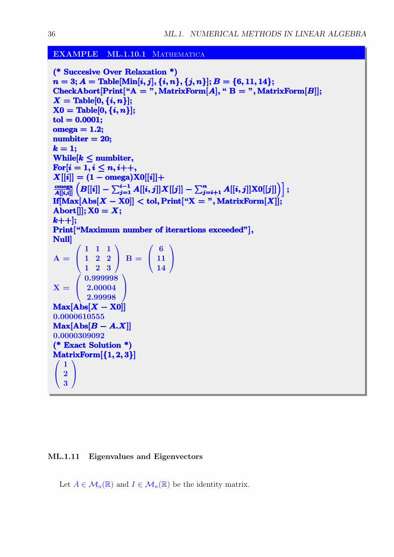
EXAMPLE ML.1.10.1 Mathematica
(* Succesive Over Relaxation *)(* Succesive Over Relaxation *)(* Succesive Over Relaxation *)n = 3; A = Table[Min[i, j], {i, n}, {j, n}]; B = {6, 11, 14};n = 3; A = Table[Min[i, j], {i, n}, {j, n}]; B = {6, 11, 14};n = 3; A = Table[Min[i, j], {i, n}, {j, n}]; B = {6, 11, 14};CheckAbort[Print[“A = ”, MatrixForm[A], “ B = ”, MatrixForm[B]];CheckAbort[Print[“A = ”, MatrixForm[A], “ B = ”, MatrixForm[B]];CheckAbort[Print[“A = ”, MatrixForm[A], “ B = ”, MatrixForm[B]];X = Table[0, {i, n}];X = Table[0, {i, n}];X = Table[0, {i, n}];X0 = Table[0, {i, n}];X0 = Table[0, {i, n}];X0 = Table[0, {i, n}];tol = 0.0001;tol = 0.0001;tol = 0.0001;omega = 1.2;omega = 1.2;omega = 1.2;numbiter = 20;numbiter = 20;numbiter = 20;k = 1;k = 1;k = 1;While[k ≤ numbiter,While[k ≤ numbiter,While[k ≤ numbiter,For[i = 1, i ≤ n, i++,For[i = 1, i ≤ n, i++,For[i = 1, i ≤ n, i++,X[[i]] = (1 − omega)X0[[i]]+X[[i]] = (1 − omega)X0[[i]]+X[[i]] = (1 − omega)X0[[i]]+omegaA[[i,i]]
(B[[i]] −
∑i−1j=1 A[[i, j]]X[[j]] −
∑nj=i+1 A[[i, j]]X0[[j]]
)];omega
A[[i,i]]
(B[[i]] −
∑i−1j=1 A[[i, j]]X[[j]] −
∑nj=i+1 A[[i, j]]X0[[j]]
)];omega
A[[i,i]]
(B[[i]] −
∑i−1j=1 A[[i, j]]X[[j]] −
∑nj=i+1 A[[i, j]]X0[[j]]
)];
If[Max[Abs[X − X0]] < tol, Print[“X = ”, MatrixForm[X]];If[Max[Abs[X − X0]] < tol, Print[“X = ”, MatrixForm[X]];If[Max[Abs[X − X0]] < tol, Print[“X = ”, MatrixForm[X]];Abort[]]; X0 = X;Abort[]]; X0 = X;Abort[]]; X0 = X;k++];k++];k++];Print[“Maximum number of iterartions exceeded”],Print[“Maximum number of iterartions exceeded”],Print[“Maximum number of iterartions exceeded”],Null]Null]Null]
A =
1 1 11 2 21 2 3
B =
61114
X =
0.9999982.000042.99998
Max[Abs[X − X0]]Max[Abs[X − X0]]Max[Abs[X − X0]]0.0000610555Max[Abs[B − A.X]]Max[Abs[B − A.X]]Max[Abs[B − A.X]]0.0000309092(* Exact Solution *)(* Exact Solution *)(* Exact Solution *)MatrixForm[{1, 2, 3}]MatrixForm[{1, 2, 3}]MatrixForm[{1, 2, 3}]
123
ML.1.11 Eigenvalues and Eigenvectors
Let A ∈Mn(R) and I ∈Mn(R) be the identity matrix.
ML.1.11. EIGENVALUES AND EIGENVECTORS 37
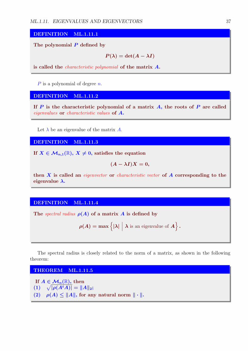
DEFINITION ML.1.11.1
The polynomial P defined by
P (λ) = det(A − λI)
is called the characteristic polynomial of the matrix A.
P is a polynomial of degree n.
DEFINITION ML.1.11.2
If P is the characteristic polynomial of a matrix A, the roots of P are calledeigenvalues or characteristic values of A.
Let λ be an eigenvalue of the matrix A.
DEFINITION ML.1.11.3
If X ∈ Mn,1(R), X 6= 0, satisfies the equation
(A − λI)X = 0,
then X is called an eigenvector or characteristic vector of A corresponding to theeigenvalue λ.
DEFINITION ML.1.11.4
The spectral radius ρ(A) of a matrix A is defined by
ρ(A) = max{
|λ|∣∣∣ λ is an eigenvalue of A
}.
The spectral radius is closely related to the norm of a matrix, as shown in the followingtheorem:
THEOREM ML.1.11.5
If A ∈ Mn(R), then(1)
√|ρ(AtA)| = ‖A‖2;
(2) ρ(A) ≤ ‖A‖, for any natural norm ‖ ∙ ‖.
38 ML.1. NUMERICAL METHODS IN LINEAR ALGEBRA
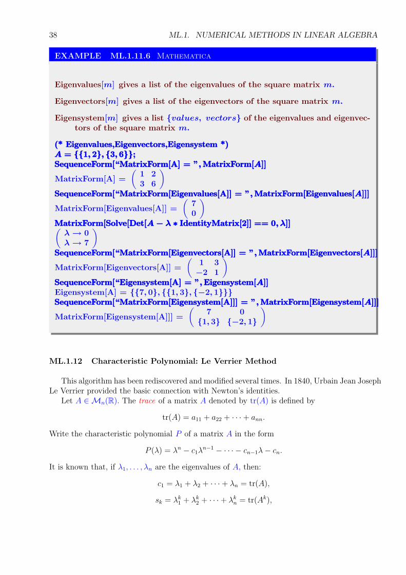
EXAMPLE ML.1.11.6 Mathematica
Eigenvalues[m] gives a list of the eigenvalues of the square matrix m.
Eigenvectors[m] gives a list of the eigenvectors of the square matrix m.
Eigensystem[m] gives a list {values, vectors} of the eigenvalues and eigenvec-tors of the square matrix m.
(* Eigenvalues,Eigenvectors,Eigensystem *)(* Eigenvalues,Eigenvectors,Eigensystem *)(* Eigenvalues,Eigenvectors,Eigensystem *)A = {{1, 2}, {3, 6}};A = {{1, 2}, {3, 6}};A = {{1, 2}, {3, 6}};SequenceForm[“MatrixForm[A] = ”, MatrixForm[A]]SequenceForm[“MatrixForm[A] = ”, MatrixForm[A]]SequenceForm[“MatrixForm[A] = ”, MatrixForm[A]]
MatrixForm[A] =
(1 23 6
)
SequenceForm[“MatrixForm[Eigenvalues[A]] = ”, MatrixForm[Eigenvalues[A]]]SequenceForm[“MatrixForm[Eigenvalues[A]] = ”, MatrixForm[Eigenvalues[A]]]SequenceForm[“MatrixForm[Eigenvalues[A]] = ”, MatrixForm[Eigenvalues[A]]]
MatrixForm[Eigenvalues[A]] =
(70
)
MatrixForm[Solve[Det[A − λ ∗ IdentityMatrix[2]] == 0, λ]]MatrixForm[Solve[Det[A − λ ∗ IdentityMatrix[2]] == 0, λ]]MatrixForm[Solve[Det[A − λ ∗ IdentityMatrix[2]] == 0, λ]](λ → 0λ → 7
)
SequenceForm[“MatrixForm[Eigenvectors[A]] = ”, MatrixForm[Eigenvectors[A]]]SequenceForm[“MatrixForm[Eigenvectors[A]] = ”, MatrixForm[Eigenvectors[A]]]SequenceForm[“MatrixForm[Eigenvectors[A]] = ”, MatrixForm[Eigenvectors[A]]]
MatrixForm[Eigenvectors[A]] =
(1 3
−2 1
)
SequenceForm[“Eigensystem[A] = ”, Eigensystem[A]]SequenceForm[“Eigensystem[A] = ”, Eigensystem[A]]SequenceForm[“Eigensystem[A] = ”, Eigensystem[A]]Eigensystem[A] = {{7, 0}, {{1, 3}, {−2, 1}}}SequenceForm[“MatrixForm[Eigensystem[A]]] = ”, MatrixForm[Eigensystem[A]]]SequenceForm[“MatrixForm[Eigensystem[A]]] = ”, MatrixForm[Eigensystem[A]]]SequenceForm[“MatrixForm[Eigensystem[A]]] = ”, MatrixForm[Eigensystem[A]]]
MatrixForm[Eigensystem[A]]] =
(7 0
{1, 3} {−2, 1}
)
ML.1.12 Characteristic Polynomial: Le Verrier Method
This algorithm has been rediscovered and modified several times. In 1840, Urbain Jean JosephLe Verrier provided the basic connection with Newton’s identities.
Let A ∈Mn(R). The trace of a matrix A denoted by tr(A) is defined by
tr(A) = a11 + a22 + ∙ ∙ ∙ + ann.
Write the characteristic polynomial P of a matrix A in the form
P (λ) = λn − c1λn−1 − ∙ ∙ ∙ − cn−1λ− cn.
It is known that, if λ1, . . . , λn are the eigenvalues of A, then:
c1 = λ1 + λ2 + ∙ ∙ ∙ + λn = tr(A),
sk = λk1 + λk
2 + ∙ ∙ ∙ + λkn = tr(Ak),
ML.1.13. CHARACTERISTIC POLYNOMIAL: FADEEV-FRAME METHOD 39
k = 1, . . . , n. Using the Newton formula
ck =1
k(sk − c1sk−1 − c2sk−2 − ∙ ∙ ∙ − ck−1s1),
k = 2, . . . , n, we obtain:
c1 = tr(A),c2 = 1
2(tr(A2)− c1tr(A)),
. . . . . . . . . . . . . . . . . . . . . . . . . . . . . . . . . . . . . . . . . . . . . .cn = 1
n(tr(An)− c1tr(A
n−1)− ∙ ∙ ∙ − cn−1tr(A)).
ML.1.13 Characteristic Polynomial: Fadeev-Frame Method
J. M. Souriau, also from France, and J. S. Frame, from Michigan State University, inde-pendently modified the algorithm to its present form. Souriau’s formulation was published inFrance in 1948, and Frame’s method appeared in the United States in 1949. Paul Horst (USA,1935) along with Faddeev and Sominskii (USSR, 1949) are also credited with rediscovering thetechnique. Although the algorithm is intriguingly beautiful, it is not practical for floating-pointcomputations. The Fadeev-Frame algorithm is closely related to the Le Verrier method.
Letdet(A− λIn) = (−1)nP (λ),
whereP (λ) = λn − c1λ
n−1 − ∙ ∙ ∙ − cn−1λ− cn.
Using the notations:
A1 = A, c1 = tr(A1), B1 = A1 − c1In,A2 = AB1, c2 = 1
2tr(A2), B2 = A2 − c2In,
......
...An = ABn−1, cn = 1
ntr(An), Bn = An − cnIn,
and taking into account the fact that the matrix A is a solution to its characteristic equation1 (Cayley -Hamilton theorem), we obtain
An − c1An−1 − ∙ ∙ ∙ − cn−1A− cnIn = P (A) = 0.
The relation Bn = An − cnIn is a control test,
Bn = 0.
Furthermore, from the relation
det(A) = (−1)nP (0) = (−1)n+1cn, (1.13.1)
1In 1896 Frobenius became aware of Cayley’s 1858 Memoir on the theory of matrices and after this startedto use the term matrix. Despite the fact that Cayley only proved the Cayley-Hamilton theorem for 2 × 2 and3× 3 matrices, Frobenius generously attributed the result to Cayley (Frobenius, in 1878, had been the first toprove the general theorem). Hamilton proved a special case of the theorem, the 4× 4 case, in the course of hisinvestigations into quaternions.
40 ML.1. NUMERICAL METHODS IN LINEAR ALGEBRA
we can determine the determinant of the matrix A.If det(A) 6= 0 then, from the relations
ABn−1 = An = cnIn,
using the formula
A−1 =1
cn
Bn−1, (1.13.2)
we obtain the inverse of the matrix A.Also, note that (−1)n+1Bn−1 is the adjoint of the matrix A.
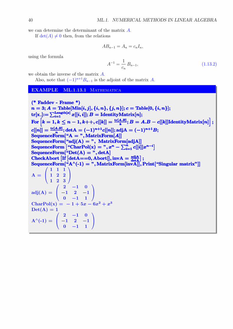
EXAMPLE ML.1.13.1 Mathematica
(* Faddev - Frame *)(* Faddev - Frame *)(* Faddev - Frame *)n = 3; A = Table[Min[i, j], {i, n}, {j, n}]; c = Table[0, {i, n}];n = 3; A = Table[Min[i, j], {i, n}, {j, n}]; c = Table[0, {i, n}];n = 3; A = Table[Min[i, j], {i, n}, {j, n}]; c = Table[0, {i, n}];
tr[x ]:=∑Length[x]i=1 x[[i, i]]; B = IdentityMatrix[n];tr[x ]:=
∑Length[x]i=1 x[[i, i]]; B = IdentityMatrix[n];tr[x ]:=
∑Length[x]i=1 x[[i, i]]; B = IdentityMatrix[n];
For[k = 1, k ≤ n − 1, k++, c[[k]] = tr[A.B]
k; B = A.B − c[[k]]IdentityMatrix[n]
];For
[k = 1, k ≤ n − 1, k++, c[[k]] = tr[A.B]
k; B = A.B − c[[k]]IdentityMatrix[n]
];For
[k = 1, k ≤ n − 1, k++, c[[k]] = tr[A.B]
k; B = A.B − c[[k]]IdentityMatrix[n]
];
c[[n]] = tr[A.B]
n; detA = (−1)n+1c[[n]]; adjA = (−1)n+1B;c[[n]] = tr[A.B]
n; detA = (−1)n+1c[[n]]; adjA = (−1)n+1B;c[[n]] = tr[A.B]
n; detA = (−1)n+1c[[n]]; adjA = (−1)n+1B;
SequenceForm[“A = ”, MatrixForm[A]]SequenceForm[“A = ”, MatrixForm[A]]SequenceForm[“A = ”, MatrixForm[A]]SequenceForm[“adj(A) = ”, MatrixForm[adjA]]SequenceForm[“adj(A) = ”, MatrixForm[adjA]]SequenceForm[“adj(A) = ”, MatrixForm[adjA]]SequenceForm
[“CharPol(x) = ”, xn −
∑ni=1 c[[i]]xn−i
]SequenceForm
[“CharPol(x) = ”, xn −
∑ni=1 c[[i]]xn−i
]SequenceForm
[“CharPol(x) = ”, xn −
∑ni=1 c[[i]]xn−i
]
SequenceForm[“Det(A) = ”, detA]SequenceForm[“Det(A) = ”, detA]SequenceForm[“Det(A) = ”, detA]CheckAbort
[If[detA==0, Abort[], invA = adjA
detA
];CheckAbort
[If[detA==0, Abort[], invA = adjA
detA
];CheckAbort
[If[detA==0, Abort[], invA = adjA
detA
];
SequenceForm[“A∧(-1) = ”, MatrixForm[invA]], Print[“Singular matrix”]]SequenceForm[“A∧(-1) = ”, MatrixForm[invA]], Print[“Singular matrix”]]SequenceForm[“A∧(-1) = ”, MatrixForm[invA]], Print[“Singular matrix”]]
A =
1 1 11 2 21 2 3
adj(A) =
2 −1 0
−1 2 −10 −1 1
CharPol(x) = − 1 + 5x − 6x2 + x3
Det(A) = 1
A∧(-1) =
2 −1 0
−1 2 −10 −1 1
ML.2
Solutions of Nonlinear Equations
ML.2.1 Introduction
In this chapter we consider one of the most basic problems in numerical approximation, theroot-finding problem.
A few type of nonlinear equations can be solved by using direct algebraic methods. Ingeneral, algebraic equations of fifth and of higher orders cannot be solved by means of radicals.Moreover, there exists no explicit formula for finding the roots of nonalgebraic (transcendental)equations such as, ex + x = 0, x ∈ R. Therefore, root-finding invariably proceeds by iteration,and this is equally true in one or in many dimensions.
Let x∗ be a real number and (xk)k≥0 be a sequence of real numbers that converges to x∗.
DEFINITION ML.2.1.1
If positive constants p and λ exist such that
limk→∞
|xk+1 − x∗|
|xk − x∗|p= λ,
then the sequence (xk)k≥0 is said to converge to x∗ of order p, with asymptoticconstant λ.
An iterative technique of the form xk+1 = f(xk), k ∈ N, is said to be of order p if thesequence (xk)k≥0 converges to the solution x∗ = f(x∗) of order p.
In general a sequence of a high order of convergence converges more rapidly than a sequencewith a lower order. Two cases of order are given special attention, namely the linear (p = 1)and the quadratic (p = 2).
Consider that ε is a bound of the maximum size of the error. We have to stop the calculationswhen the following condition is satisfied
|xk − x∗| < ε.
41
42 ML.2. SOLUTIONS OF NONLINEAR EQUATIONS
But such a criterion cannot be used because the root x∗ is not known. A typical stoppingcriterion is to stop when the difference between two successive iterates satisfy the inequality
|xk − xk+1| < ε,
We can also use as stopping criterion
|xk − xk+1| ≤ ε|xk|,
etc.
Unfortunately none of these criteria guarantees the required precision.
The following section deals with several traditional iterative methods.
ML.2.2 Method of Successive Approximation
Let F : [a, b]→ R be a function. A number x is said to be a fixed point of the function F if
F (x) = x.
Root-finding problems and fixed-point problems are equivalent classes in the following sense:
A point x is a root of the equation
f(x) = 0
if and only if it is a fixed point of the function
F (x) = x− f(x).
Although the problem we wish to solve is in the root-finding form, the fixed-point form is easierto analyze and certain fixed-point choices lead to very powerful root-finding techniques.
THEOREM ML.2.2.1
If F : [a, b] → [a, b] has derivative such that |F ′(x)| ≤ α < 1, for all x ∈ (a, b),then the function F has a unique fixed point x∗, and the sequence (xk)k>0,defined by:
xk+1 = F (xk), k ∈ N, x0 ∈ [a, b].
converges to x∗.
Proof. Using Lagrange’s mean value theorem it follows that for all x, y ∈ [a, b] there existsc ∈ (a, b) such that
|F (x)− F (y)| = |F ′(c)| ∙ |x− y| ≤ α|x− y|.
The function F is a contraction. The proof is concluded by using the Banach fixed pointtheorem.
ML.2.3. THE BISECTION METHOD 43
THEOREM ML.2.2.2
Let F ∈ Cp[a, b], p ≥ 2, and x∗ ∈ (a, b) be a fixed point of F . If
F ′(x∗) = F ′′(x∗) = ∙ ∙ ∙ = F (p−1)(x∗) = 0, F (p)(x∗) 6= 0,
then, for x0 sufficiently close to x∗, the sequence (xk)k>0, where
xk+1 = F (xk), k ∈ N, x0 ∈ [a, b],
converges to x∗, of order p.
Proof. Since |F ′(x∗)| = 0 < 1, there exists a ball centered at x∗ on which F be a contraction.By virtue of Banach’s fixed point theorem it follows that the sequence (xk)k≥0 converges to x∗.Using Taylor’s formula it follows that there exists ck ∈ (a, b) such that
xk+1 = F (xk)
= F (x∗) +
p−1∑
i=1
F (i)(x∗)(xk − x∗)i
i!+ F (p)(ck)
(xk − x∗)p
p!
= x∗ + 0 + F (p)(ck)(xk − x∗)p
p!,
hence
limk→∞
|xk+1 − x∗||xk − x∗|p
= limk→∞
|F (p)(ck)|p!
=|F (p)(x∗)|
p!> 0.
Consequently, the method has order p.
ML.2.3 The Bisection Method
THEOREM ML.2.3.1
If f ∈ C[a, b] and f(a)f(b) < 0 then the sequence (xk)k≥0, defined by:x0 = a, y0 = b;
xk+1, yk+1 ∈
{
xk,xk + yk
2, yk
}
, such that:
yk+1 − xk+1 =yk − xk
2,
f(xk+1)f(yk+1) ≤ 0, k ∈ N,converges to a root x∗ of the equation f(x) = 0. Moreover, we have
|xk − x∗| ≤b − a
2k, k ∈ N.
Proof. The sequence (xk)k≥0 is increasing, the sequence (yk)k≥0 is decreasing such thatyk−xk → 0. It follows that they converge to the same limit x∗. From the conditions f(xk)f(yk) ≤
44 ML.2. SOLUTIONS OF NONLINEAR EQUATIONS
0, k →∞, we deduce
f 2(x∗) ≤ 0,
that is
f(x∗) = 0.
Since
yk − xk =b− a
2k,
it follows that
|xk − x∗| ≤b− a
2k.
This is only a bound for the arising error in approximation process. The actual error can bemuch smaller.
The bisection method, is also called the binary-search method. It is very slow in converging.However, the method guarantees convergence to a solution and, for this reason, it is used as a“starter” for more efficient methods.
ML.2.4 The Newton-Raphson Method
The Newton-Raphson method (or simply Newton’s method) is one of the most powerful andwell-known techniques used for a root-finding problem.
THEOREM ML.2.4.1
If x0 ∈ [a, b] and f ∈ C2[a, b] satisfies the conditions:(1) f(a)f(b) < 0;
(2) f ′ and f ′′ have no roots in [a, b],
(3) f(x0)f′′(x0) > 0,
then the equation f(x) = 0 has a unique solution x∗ ∈ (a, b), and the sequence(xk)k≥0 defined by
xk+1 = xk − f(xk)/f ′(xk), k ∈ N,
converges to x∗.
We shall prove that the Newton method is of order 2. Indeed, using Taylor’s formula, wehave
0 = f(x∗) = f(xk) + (x∗ − xk)f′(xk) + (x∗ − xk)
2 f ′′(ck)
2,
where |x∗ − ck| ≤ |x∗ − xk|, which we rewrite in the form
xk+1 − x∗ = (x∗ − xk)2 f ′′(ck)
2f ′(xk),
ML.2.5. THE SECANT METHOD 45
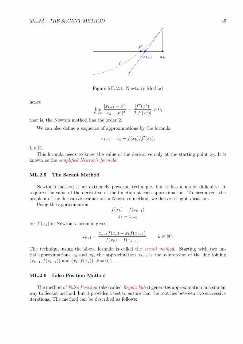
������������
•••x∗
xk+1 xk
f
Figure ML.2.1: Newton’s Method
hence
limk→∞
|xk+1 − x∗||xk − x∗|2
=|f ′′(x∗)|2|f ′(x∗)|
> 0,
that is, the Newton method has the order 2.
We can also define a sequence of approximations by the formula
xk+1 = xk − f(xk)/f′(x0),
k ∈ N.This formula needs to know the value of the derivative only at the starting point x0. It is
known as the simplified Newton’s formula.
ML.2.5 The Secant Method
Newton’s method is an extremely powerful technique, but it has a major difficulty: itrequires the value of the derivative of the function at each approximation. To circumvent theproblem of the derivative evaluation in Newton’s method, we derive a slight variation.
Using the approximationf(xk)− f(xk−1)
xk − xk−1
for f ′(xk) in Newton’s formula, gives
xk+1 =xk−1f(xk)− xkf(xk−1)
f(xk)− f(xk−1), k ∈ N∗.
The technique using the above formula is called the secant method. Starting with two ini-tial approximations x0 and x1, the approximation xk+1 is the x-intercept of the line joining(xk−1, f(xk−1)) and (xk, f(xk)), k = 0, 1, . . .
ML.2.6 False Position Method
The method of False Position (also called Regula Falsi) generates approximation in a similarway to Secant method, but it provides a test to ensure that the root lies between two successiveiterations. The method can be described as follows:
46 ML.2. SOLUTIONS OF NONLINEAR EQUATIONS
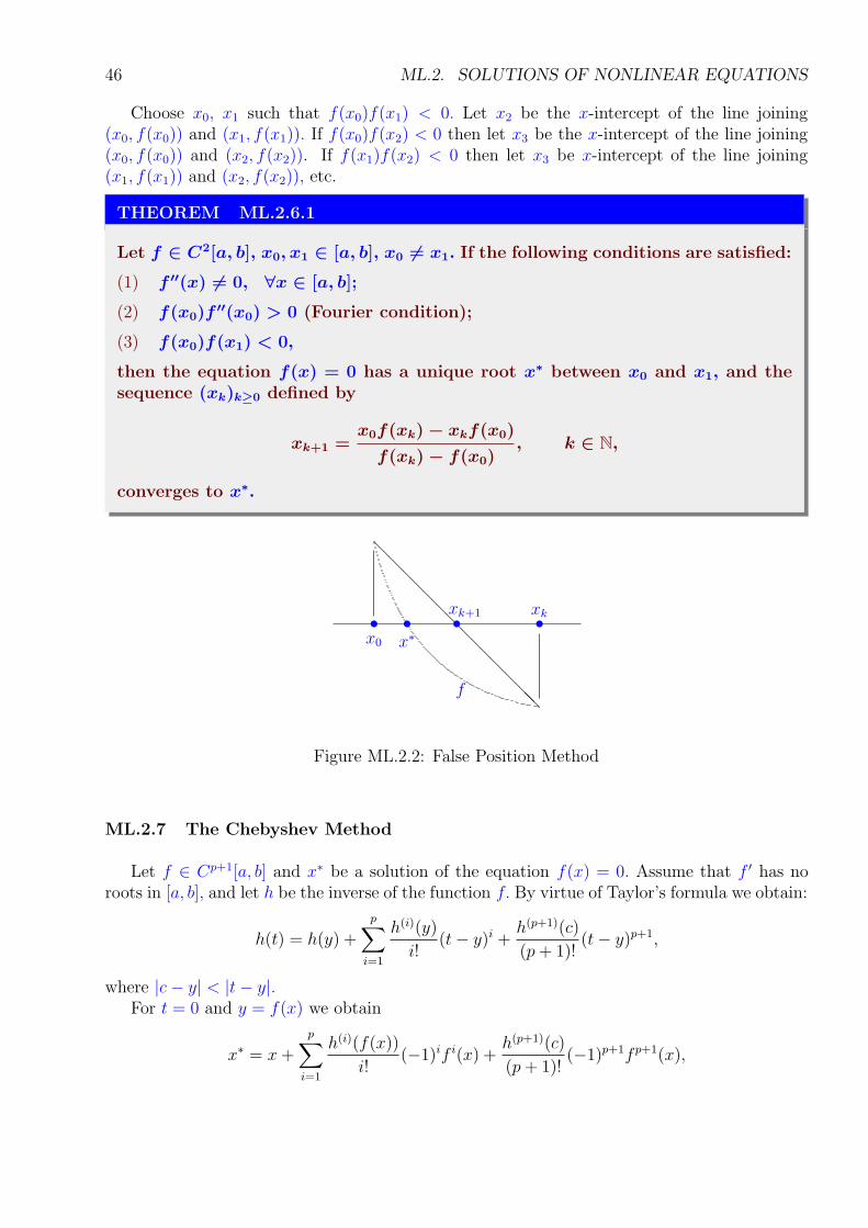
Choose x0, x1 such that f(x0)f(x1) < 0. Let x2 be the x-intercept of the line joining(x0, f(x0)) and (x1, f(x1)). If f(x0)f(x2) < 0 then let x3 be the x-intercept of the line joining(x0, f(x0)) and (x2, f(x2)). If f(x1)f(x2) < 0 then let x3 be x-intercept of the line joining(x1, f(x1)) and (x2, f(x2)), etc.
THEOREM ML.2.6.1
Let f ∈ C2[a, b], x0, x1 ∈ [a, b], x0 6= x1. If the following conditions are satisfied:
(1) f ′′(x) 6= 0, ∀x ∈ [a, b];
(2) f(x0)f′′(x0) > 0 (Fourier condition);
(3) f(x0)f(x1) < 0,
then the equation f(x) = 0 has a unique root x∗ between x0 and x1, and thesequence (xk)k≥0 defined by
xk+1 =x0f(xk) − xkf(x0)
f(xk) − f(x0), k ∈ N,
converges to x∗.
@@@@@@@@@@@@
x0 x∗
xk+1 xk• • • •
f
Figure ML.2.2: False Position Method
ML.2.7 The Chebyshev Method
Let f ∈ Cp+1[a, b] and x∗ be a solution of the equation f(x) = 0. Assume that f ′ has noroots in [a, b], and let h be the inverse of the function f. By virtue of Taylor’s formula we obtain:
h(t) = h(y) +
p∑
i=1
h(i)(y)
i!(t− y)i +
h(p+1)(c)
(p + 1)!(t− y)p+1,
where |c− y| < |t− y|.For t = 0 and y = f(x) we obtain
x∗ = x +
p∑
i=1
h(i)(f(x))
i!(−1)if i(x) +
h(p+1)(c)
(p + 1)!(−1)p+1f p+1(x),
ML.2.7. THE CHEBYSHEV METHOD 47
where |c− f(x)| ≤ |f(x)|. Using the notation
F (x) = x +
p∑
i=1
(−1)i
i!ai(x)f i(x),
where ai(x) = h(i)(f(x)).
The Chebyshev method can be obtained by defining the sequence (xk)k≥0 such that
xk+1 = F (xk), k ∈ N.
If h(p+1)(0) 6= 0, then the Chebyshev method has the order of convergence p + 1.
In order to calculate the coefficients ai(x), i = 1, . . . , p, we differentiate p-times, the identity
h(f(x)) = x, ∀x ∈ [a, b].
We obtain:
h′(f(x)) ∙ f ′(x) = 1,
i.e.,
a1(x)f ′(x) = 1, a1(x) =1
f ′(x),
and
ai =1
f ′(x)
d
dxai−1(x), i = 1, . . . p,
where a0(x) = x.
For p = 1 we obtain
xk+1 = xk − f(xk)/f′(xk),
k ∈ N, i.e., the Newton method.
For p = 2 we obtain a Chebyshev method of order 3:
xk+1 = xk −f(xk)
f ′(xk)−
f ′′(xk)f2(xk)
2(f ′(xk))3,
k ∈ N.
The Chebyshev method needs more calculations, but it converges more rapidly.
48 ML.2. SOLUTIONS OF NONLINEAR EQUATIONS
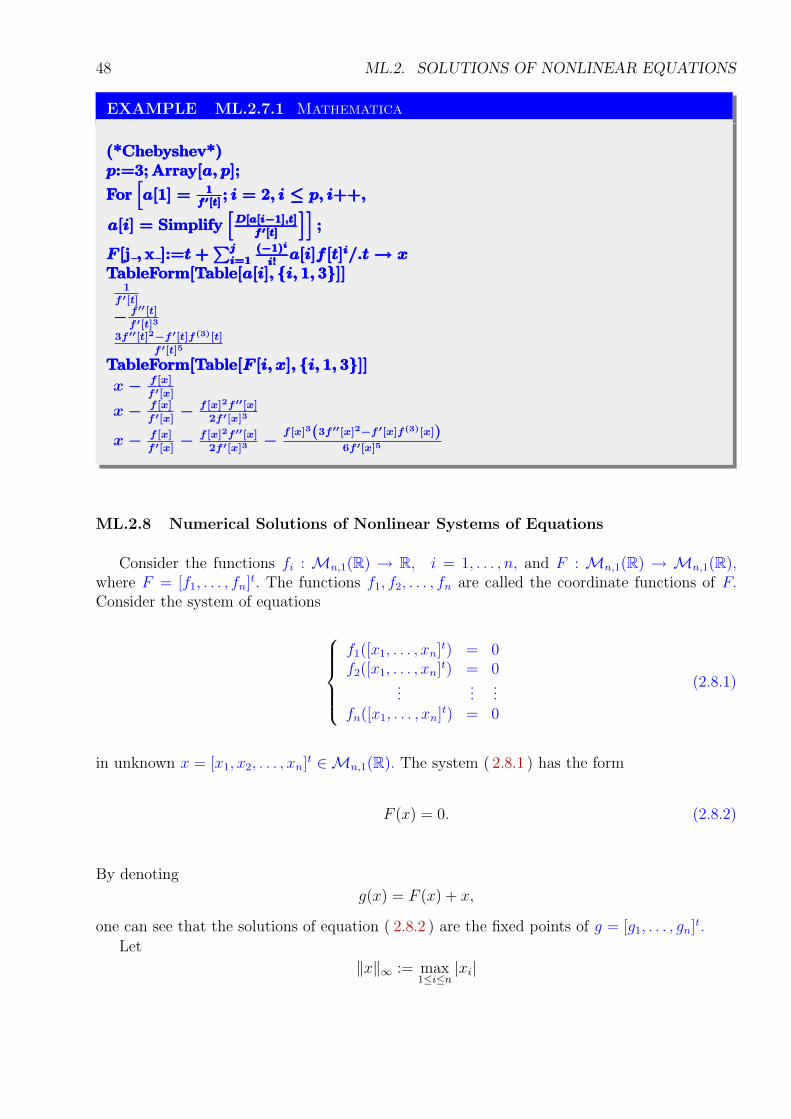
EXAMPLE ML.2.7.1 Mathematica
(*Chebyshev*)(*Chebyshev*)(*Chebyshev*)p:=3; Array[a, p];p:=3; Array[a, p];p:=3; Array[a, p];
For[a[1] = 1
f ′[t]; i = 2, i ≤ p, i++,For
[a[1] = 1
f ′[t]; i = 2, i ≤ p, i++,For
[a[1] = 1
f ′[t]; i = 2, i ≤ p, i++,
a[i] = Simplify[D[a[i−1],t]
f ′[t]
]];a[i] = Simplify
[D[a[i−1],t]
f ′[t]
]];a[i] = Simplify
[D[a[i−1],t]
f ′[t]
]];
F [j , x ]:=t +∑ji=1
(−1)i
i!a[i]f [t]i/.t → xF [j , x ]:=t +
∑ji=1
(−1)i
i!a[i]f [t]i/.t → xF [j , x ]:=t +
∑ji=1
(−1)i
i!a[i]f [t]i/.t → x
TableForm[Table[a[i], {i, 1, 3}]]TableForm[Table[a[i], {i, 1, 3}]]TableForm[Table[a[i], {i, 1, 3}]]1f ′[t]
− f ′′[t]
f ′[t]3
3f ′′[t]2−f ′[t]f(3)[t]
f ′[t]5
TableForm[Table[F [i, x], {i, 1, 3}]]TableForm[Table[F [i, x], {i, 1, 3}]]TableForm[Table[F [i, x], {i, 1, 3}]]
x − f [x]
f ′[x]
x − f [x]
f ′[x]− f [x]2f ′′[x]
2f ′[x]3
x − f [x]
f ′[x]− f [x]2f ′′[x]
2f ′[x]3−f [x]3(3f ′′[x]2−f ′[x]f(3)[x])
6f ′[x]5
ML.2.8 Numerical Solutions of Nonlinear Systems of Equations
Consider the functions fi : Mn,1(R) → R, i = 1, . . . , n, and F : Mn,1(R) → Mn,1(R),where F = [f1, . . . , fn]t. The functions f1, f2, . . . , fn are called the coordinate functions of F.Consider the system of equations
f1([x1, . . . , xn]t) = 0f2([x1, . . . , xn]t) = 0
......
...fn([x1, . . . , xn]t) = 0
(2.8.1)
in unknown x = [x1, x2, . . . , xn]t ∈Mn,1(R). The system ( 2.8.1 ) has the form
F (x) = 0. (2.8.2)
By denoting
g(x) = F (x) + x,
one can see that the solutions of equation ( 2.8.2 ) are the fixed points of g = [g1, . . . , gn]t.
Let
‖x‖∞ := max1≤i≤n
|xi|
ML.2.9. NEWTON’S METHOD FOR SYSTEMS OF NONLINEAR EQUATIONS 49
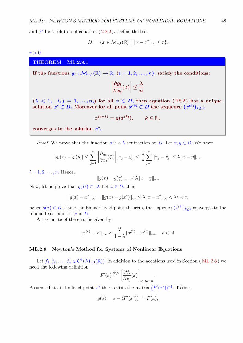
and x∗ be a solution of equation ( 2.8.2 ). Define the ball
D := {x ∈Mn,1(R) | ‖x− x∗‖∞ ≤ r},
r > 0.
THEOREM ML.2.8.1
If the functions gi : Mn,1(R) → R, (i = 1, 2, . . . , n), satisfy the conditions:
∣∣∣∣∂gi
∂xj(x)
∣∣∣∣ ≤
λ
n
(λ < 1, i, j = 1, . . . , n,) for all x ∈ D, then equation ( 2.8.2 ) has a uniquesolution x∗ ∈ D. Moreover for all point x(0) ∈ D the sequence (x(k))k≥0,
x(k+1) = g(x(k)), k ∈ N,
converges to the solution x∗.
Proof. We prove that the function g is a λ-contraction on D. Let x, y ∈ D. We have:
|gi(x)− gi(y)| ≤n∑
j=1
∣∣∣∣∂gi
∂xj
(ξi)
∣∣∣∣ |xj − yj| ≤
λ
n
n∑
j=1
|xj − yj| ≤ λ‖x− y‖∞,
i = 1, 2, . . . , n. Hence,‖g(x)− g(y)‖∞ ≤ λ‖x− y‖∞.
Now, let us prove that g(D) ⊂ D. Let x ∈ D, then
‖g(x)− x∗‖∞ = ‖g(x)− g(x∗)‖∞ ≤ λ‖x− x∗‖∞ < λr < r,
hence g(x) ∈ D. Using the Banach fixed point theorem, the sequence (x(k))k≥0 converges to theunique fixed point of g in D.
An estimate of the error is given by
‖x(k) − x∗‖∞ <λk
1− λ‖x(1) − x(0)‖∞, k ∈ N.
ML.2.9 Newton’s Method for Systems of Nonlinear Equations
Let f1, f2, . . . , fn ∈ C1(Mn,1(R)). In addition to the notations used in Section ( ML.2.8 ) weneed the following definition
F ′(x)def.=
[∂fi
∂xj
(x)
]
1≤i,j≤n
.
Assume that at the fixed point x∗ there exists the matrix (F ′(x∗))−1. Taking
g(x) = x− (F ′(x∗))−1 ∙ F (x),
50 ML.2. SOLUTIONS OF NONLINEAR EQUATIONS
we can see that∂gi
∂xj
(x∗) = 0,
i, j = 1, 2, . . . , n. Since F is continuous, there exists a ball D centered at x∗ such that theconditions of Theorem ( ML.2.8.1 ) are satisfied for
g(x) = x− (F ′(x))−1 ∙ F (x).
For a certain value x0, sufficiently close to x∗, the sequence (x(k))k≥0, defined by
x(k+1) = x(k) − (F ′(x(k)))−1 ∙ F (x(k)), k ∈ N,
converges to x∗.
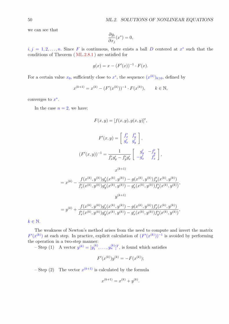
In the case n = 2, we have:
F (x, y) = [f(x, y), g(x, y)]t,
F ′(x, y) =
[f ′
x f ′y
g′x g′
y
]
,
(F ′(x, y))−1 =1
f ′xg
′y − f ′
yg′x
[g′
y −f ′y
−g′x f ′
x
]
,
x(k+1)
= x(k) −f(x(k), y(k))g′
y(x(k), y(k))− g(x(k), y(k))f ′
y(x(k), y(k))
f ′x(x
(k), y(k))g′y(x
(k), y(k))− g′x(x
(k), y(k))f ′y(x
(k), y(k)),
y(k+1)
= y(k) +f(x(k), y(k))g′
x(x(k), y(k))− g(x(k), y(k))f ′
x(x(k), y(k))
f ′x(x
(k), y(k))g′y(x
(k), y(k))− g′x(x
(k), y(k))f ′y(x
(k), y(k)),
k ∈ N.
The weakness of Newton’s method arises from the need to compute and invert the matrixF ′(x(k)) at each step. In practice, explicit calculation of (F ′(x(k)))−1 is avoided by performingthe operation in a two-step manner:
– Step (1) A vector y(k) = [y(k)1 , . . . , y
(k)n ]T , is found which satisfies
F ′(x(k))y(k) = −F (x(k));
– Step (2) The vector x(k+1) is calculated by the formula
x(k+1) = x(k) + y(k).
ML.2.10. STEEPEST DESCENT METHOD 51
ML.2.10 Steepest Descent Method
The steepest descent method (also called the gradient method) determines a local minimumfor a function Ψ : Rn → R. Note that the system ( 2.8.1 ) has a solution precisely when thefunction Ψ defined by
Ψ = f 21 + ∙ ∙ ∙ + f 2
n
has the minimal value zero.The method of Steepest Descent for finding a local minimum for an arbitrary function
Ψ : Rn → R can be intuitively described as follows:
(1) Evaluate Ψ at an initial approximation x(0);
(2) Determine a direction from x(0) that results in a decrease in the value of Ψ;
(3) Move an appropriate distance in this direction and call the new vector x(1);
Repeat steps (1) to (3).More precisely:Consider a starting value x(0). Find the minimum of the function
t 7→ Ψ(x(0) − t grad Ψ(x(0))).
Let t0 be the smallest positive root of the equation
d
dt(Ψ(x(0) − t grad Ψ(x(0)))) = 0.
Definex(1) = x(0) − t0 grad Ψ(x(0)),
and, step by step, denoting by tk the smallest nonnegative root of the equation
d
dt(Ψ(x(k) − t grad Ψ(x(k)))) = 0,
takex(k+1) = x(k) − tk grad Ψ(x(k)), k ∈ N.
The Steepest Descent converges only linearly. As a consequence, the method is used to findsufficiently accurate starting approximation for the Newton based techniques.

52
ML.3
Elements of Interpolation Theory
Sometimes we know the values of a function f at a set of numbers x0 < ∙ ∙ ∙ < xn, but we donot have an analytic expression for f. For example, the values f(xi) might be obtained fromsome physical measurement. The task now is to estimate f(x) for an arbitrary x.
If the required x lies in the interval (x0, xn) the problem is called interpolation; if x isoutside the interval [x0, xn], it is called extrapolation. Interpolation must model the functionby some known function called interpolator. By far most common among the functions used asinterpolators are polynomials. Rational functions and trigonometric polynomials also turn outto be extremely useful in interpolation.
We would like to emphasize the contribution given to the Interpolation Theory by themembers of the school of thought in the Theory of Allure, Convexity and Interpolation foundedby Elena Popoviciu.
ML.3.1 Lagrange Interpolation
Let x0 < ∙ ∙ ∙ < xn be a set of distinct real numbers and f be a function whose values aregiven at these numbers.
DEFINITION ML.3.1.1
The polynomial P of degree at most n such that
P (xi) = f(xi), i = 0, . . . , n,
is called the Lagrange Interpolating Polynomial (or simply, Lagrange Polynomial)of the function f with respect to x0, . . . , xn.
The numbers xi are called mesh points or interpolation points.
Consider the polynomial P : R→ R, P (x) = a0 + a1x + ∙ ∙ ∙ + anxn. The Lagrange interpo-lating conditions
P (xi) = f(xi), i = 0, . . . , n,
53
54 ML.3. ELEMENTS OF INTERPOLATION THEORY
are equivalent to the system
a0 + a1x0 + ∙ ∙ ∙+ anxn0 = f(x0)
a0 + a1x1 + ∙ ∙ ∙+ anxn1 = f(x1)
......
......
a0 + a1xn + ∙ ∙ ∙+ anxnn = f(xn)
in unknowns a0, . . . , an.Since the Vandermonde determinant
V (x0, . . . , xn) =
∣∣∣∣∣∣∣∣∣
1 x0 ∙ ∙ ∙ xn0
1 x1 ∙ ∙ ∙ xn1
......
. . ....
1 xn ∙ ∙ ∙ xnn
∣∣∣∣∣∣∣∣∣
is different from zero (the points xi are distinct) the above system has a unique solution. Theuniqueness of the Lagrange Polynomial allows us to denote it by the symbol
L(x0, . . . , xn; f).
DEFINITION ML.3.1.2
The divided difference of the function f with respect to the points x0, . . . , xn,is defined to be the coefficient at xn in the Lagrange interpolating polynomialL(x0, . . . , xn; f) and is denoted by
[x0, . . . , xn; f ].
For example,
[x0; f ] = f(x0), [x0, x1; f ] =f(x1)− f(x0)
x1 − x0
.
REMARK ML.3.1.3
In the case when the points xi are not distinct, see ( ML.3.6.2 ). For instance,
[x0, x0, x0; f ] =f ′′(x0)
2.
ML.3.2 Some Forms of the Lagrange Polynomial
From the interpolating conditions:
L(x0, . . . , xn; f)(xi) = f(xi), i = 0, . . . , n,
ML.3.2. SOME FORMS OF THE LAGRANGE POLYNOMIAL 55
we obtain the system
a0 + a1x0 + ∙ ∙ ∙+ anxn0 = f(x0)
a0 + a1x1 + ∙ ∙ ∙+ anxn1 = f(x1)
......
......
a0 + a1xn + ∙ ∙ ∙+ anxnn = f(xn)
a0 + a1x + ∙ ∙ ∙+ anxn = L(x0, . . . , xn; f)(x)
in unknowns a0, . . . , an. The system has a solution if∣∣∣∣∣∣∣∣∣∣∣
1 x0 ∙ ∙ ∙ xn0 f(x0)
1 x1 ∙ ∙ ∙ xn1 f(x1)
......
. . ....
...1 xn ∙ ∙ ∙ xn
n f(xn)1 x ∙ ∙ ∙ xn L(x0, . . . , xn; f)(x)
∣∣∣∣∣∣∣∣∣∣∣
= 0,
hence, we obtain
L(x0, . . . , xn; f)(x) = −
∣∣∣∣∣∣∣∣∣∣∣
1 x0 ∙ ∙ ∙ xn0 f(x0)
1 x1 ∙ ∙ ∙ xn1 f(x1)
......
. . ....
...1 xn ∙ ∙ ∙ xn
n f(xn)1 x ∙ ∙ ∙ xn 0
∣∣∣∣∣∣∣∣∣∣∣
V (x0, . . . , xn)(3.2.1)
Consider the polynomials `i ∈ R[X], i = 0, . . . , n,
`i(x) =(x− x0) . . . (x− xi−1)(x− xi+1) . . . (x− xn)
(xi − x0) . . . (xi − xi−1)(xi − xi+1) . . . (xi − xn).
It is clear that:`i(xk) = δik, i, k = 0, . . . n,
and hence the polynomial
P =n∑
i=0
f(xi)`i
satisfies the relations:P (xk) = f(xk), k = 0, . . . , n.
Since the Lagrange Polynomial has a unique representation we obtain P = L(x0, . . . , xn; f).Hence
L(x0, . . . , xn; f) =n∑
i=0
f(xi)`i. (3.2.2)
The polynomials `i are called the fundamental polynomials of the Lagrange interpolation. Byletting
`(x) = (x− x0)(x− x1) . . . (x− xn),
56 ML.3. ELEMENTS OF INTERPOLATION THEORY
we obtain
`i(x) =`(x)
(x− xi)`′(xi),
and consequently
L(x0, . . . , xn; f)(x) =n∑
i=0
f(xi)`(x)
(x− xi)`′(xi). (3.2.3)
Consider the polynomial
Q = L(x0, . . . , xn; f)− (X − x0) . . . (X − xn−1)[x0, . . . , xn; f ].
Note that the polynomial Q is of degree at most n− 1 and it satisfies the relations:
Q(xi) = f(xi), i = 0, . . . , n − 1.
It follows thatQ = L(x0, . . . , xn−1; f),
and henceL(x0, . . . , xn; f)
= L(x0, . . . , xn−1; f) + (X − x0) . . . (X − xn−1)[x0, . . . , xn; f ].
Adding the equalities:
L(x0, x1; f) = f(x0) + (X − x0)[x0, x1; f ]L(x0, x1, x2; f) = L(x0, x1; f) + (X − x0)(X − x1)[x0, x1, x2; f ]. . . . . . . . . . . . . . . . . . . . . . . . . . . . . . . . . . . . . . . . . . . . . . . . . . . . . . . . . . . . . .L(x0, . . . , xn; f) = L(x0, . . . , xn−1; f)
+(X − x0) . . . (X − xn−1)[x0, . . . , xn; f ],
we obtain the Newton Interpolatory Divided Difference Formula:
L(x0, . . . , xn; f)= f(x0) + (X − x0)[x0, x1; f ] + ∙ ∙ ∙
+(X − x0) . . . (X − xn−1)[x0, . . . , xn; f ].(3.2.4)
EXAMPLE ML.3.2.1
L(x0, x1; f) = −
∣∣∣∣∣∣
1 x0 f(x0)1 x1 f(x1)1 x 0
∣∣∣∣∣∣
/
∣∣∣∣
1 x0
1 x1
∣∣∣∣
=x − x1
x0 − x1
f(x0) +x − x0
x1 − x0
f(x1)
= f(x0) + (x − x0)[x0, x1; f ].
ML.3.2. SOME FORMS OF THE LAGRANGE POLYNOMIAL 57
Let xi, xj be distinct points, i, j ∈ {0, . . . , n}. Let
Lk := L(x0, . . . , xk−1, xk+1, . . . , xn; f), k = 0, . . . , n.
Consider the polynomial
Q =(X − xi)Li − (X − xj)Lj
xj − xi
.
Note that:
Q(xi) = −xi − xj
xj − xi
Lj(xi) = f(xi),
Q(xj) =xj − xi
xj − xi
Li(xj) = f(xj),
Q(xk) =(xk − xi)f(xk)− (xk − xj)f(xk)
xj − xi
= f(xk),
k ∈ {0, . . . , n} \ {i, j}, that is,
Q(xk) = f(xk), k = 0, . . . , n,
and grad (Q) ≤ n. Hence,Q = L(x0, . . . , xn; f).
Consequently we obtain the Aitken-Neville formula:
L(x0, . . . , xn; f) =X − xi
xj − xi
L(x0, . . . , xi−1, xi+1, . . . , xn; f)
−X − xj
xj − xi
L(x0, . . . , xj−1, xj+1, . . . , xn; f)
(i, j ∈ {0, . . . , n}, i 6= j).
(3.2.5)
Consider the notations:
Q(i, j) = L(xi−j , . . . , xi; f)(x), 0 ≤ j ≤ i ≤ n.
Using formula ( 3.2.5 ) we obtain the following algorithm
Q(i, j) =(x− xi−j)Q(i, j − 1)− (x− xi)Q(i− 1, j − 1)
xi − xi−j
(i = 1, . . . , n; j = 1, . . . , i).(3.2.6)
used to generate recursively the Lagrange Polynomials.
For example, with n = 3, the polynomials can be obtained by proceeding as shown in the tablebelow, where each row is completed before the succeeding rows are begun.
Q(0, 0) = f(x0)↓
Q(1, 0) = f(x1) Q(1, 1)↓
Q(2, 0) = f(x2) Q(2, 1) → Q(2, 2)↙
Q(3, 0) = f(x3) Q(3, 1) → Q(3, 2) → Q(3, 3)
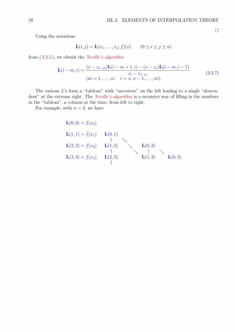
58 ML.3. ELEMENTS OF INTERPOLATION THEORY
Using the notations
L(i, j) = L(xi, . . . , xj; f)(x) (0 ≤ i ≤ j ≤ n)
from ( 3.2.5 ), we obtain the Neville’s algorithm
L(i−m, i) =(x− xi−m)L(i−m + 1, i)− (x− xi)L(i−m, i− 1)
xi − xi−m
(m = 1, . . . , n; i = n, n− 1, . . . ,m).(3.2.7)
The various L’s form a “tableau” with “ancestors” on the left leading to a single “descen-dent” at the extreme right. The Neville’s algorithm is a recursive way of filling in the numbersin the “tableau”, a column at the time, from left to right.
For example, with n = 3, we have
L(0, 0) = f(x0)
L(1, 1) = f(x1) L(0, 1)↑ ↘
L(2, 2) = f(x2) L(1, 2) ↘ L(0, 2)↑ ↘ ↑ ↘
L(3, 3) = f(x3) L(2, 3) L(1, 3) L(0, 3)↑
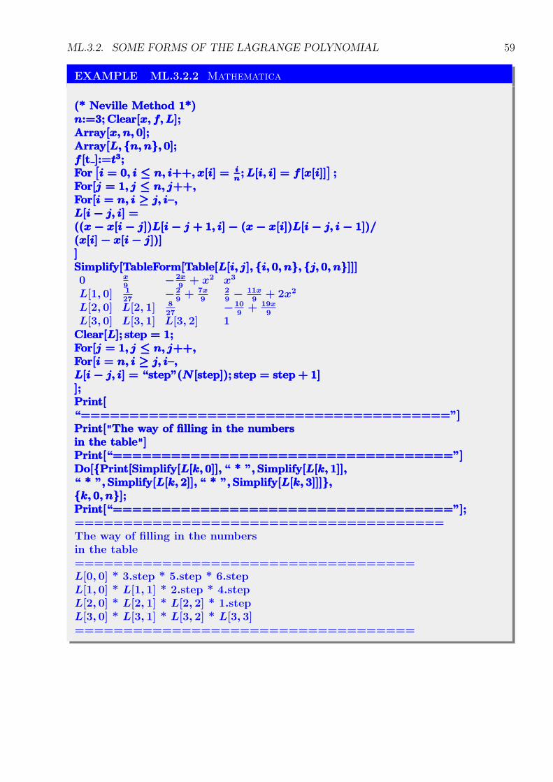
ML.3.2. SOME FORMS OF THE LAGRANGE POLYNOMIAL 59
EXAMPLE ML.3.2.2 Mathematica
(* Neville Method 1*)(* Neville Method 1*)(* Neville Method 1*)n:=3; Clear[x, f, L];n:=3; Clear[x, f, L];n:=3; Clear[x, f, L];Array[x, n, 0];Array[x, n, 0];Array[x, n, 0];Array[L, {n, n}, 0];Array[L, {n, n}, 0];Array[L, {n, n}, 0];f [t ]:=t3;f [t ]:=t3;f [t ]:=t3;For
[i = 0, i ≤ n, i++, x[i] = i
n; L[i, i] = f [x[i]]
];For
[i = 0, i ≤ n, i++, x[i] = i
n; L[i, i] = f [x[i]]
];For
[i = 0, i ≤ n, i++, x[i] = i
n; L[i, i] = f [x[i]]
];
For[j = 1, j ≤ n, j++,For[j = 1, j ≤ n, j++,For[j = 1, j ≤ n, j++,For[i = n, i ≥ j, i–,For[i = n, i ≥ j, i–,For[i = n, i ≥ j, i–,L[i − j, i] =L[i − j, i] =L[i − j, i] =((x − x[i − j])L[i − j + 1, i] − (x − x[i])L[i − j, i − 1])/((x − x[i − j])L[i − j + 1, i] − (x − x[i])L[i − j, i − 1])/((x − x[i − j])L[i − j + 1, i] − (x − x[i])L[i − j, i − 1])/(x[i] − x[i − j])](x[i] − x[i − j])](x[i] − x[i − j])]]]]Simplify[TableForm[Table[L[i, j], {i, 0, n}, {j, 0, n}]]]Simplify[TableForm[Table[L[i, j], {i, 0, n}, {j, 0, n}]]]Simplify[TableForm[Table[L[i, j], {i, 0, n}, {j, 0, n}]]]0 x
9−2x
9+ x2 x3
L[1, 0] 127
−29
+ 7x9
29
− 11x9
+ 2x2
L[2, 0] L[2, 1] 827
−109
+ 19x9
L[3, 0] L[3, 1] L[3, 2] 1Clear[L]; step = 1;Clear[L]; step = 1;Clear[L]; step = 1;For[j = 1, j ≤ n, j++,For[j = 1, j ≤ n, j++,For[j = 1, j ≤ n, j++,For[i = n, i ≥ j, i–,For[i = n, i ≥ j, i–,For[i = n, i ≥ j, i–,L[i − j, i] = “step”(N [step]); step = step + 1]L[i − j, i] = “step”(N [step]); step = step + 1]L[i − j, i] = “step”(N [step]); step = step + 1]];];];Print[Print[Print[“======================================”]“======================================”]“======================================”]Print["The way of filling in the numbersPrint["The way of filling in the numbersPrint["The way of filling in the numbersin the table"]in the table"]in the table"]Print[“===================================”]Print[“===================================”]Print[“===================================”]Do[{Print[Simplify[L[k, 0]], “ * ”, Simplify[L[k, 1]],Do[{Print[Simplify[L[k, 0]], “ * ”, Simplify[L[k, 1]],Do[{Print[Simplify[L[k, 0]], “ * ”, Simplify[L[k, 1]],“ * ”, Simplify[L[k, 2]], “ * ”, Simplify[L[k, 3]]]},“ * ”, Simplify[L[k, 2]], “ * ”, Simplify[L[k, 3]]]},“ * ”, Simplify[L[k, 2]], “ * ”, Simplify[L[k, 3]]]},{k, 0, n}];{k, 0, n}];{k, 0, n}];Print[“===================================”];Print[“===================================”];Print[“===================================”];======================================The way of filling in the numbersin the table===================================L[0, 0] * 3.step * 5.step * 6.stepL[1, 0] * L[1, 1] * 2.step * 4.stepL[2, 0] * L[2, 1] * L[2, 2] * 1.stepL[3, 0] * L[3, 1] * L[3, 2] * L[3, 3]===================================
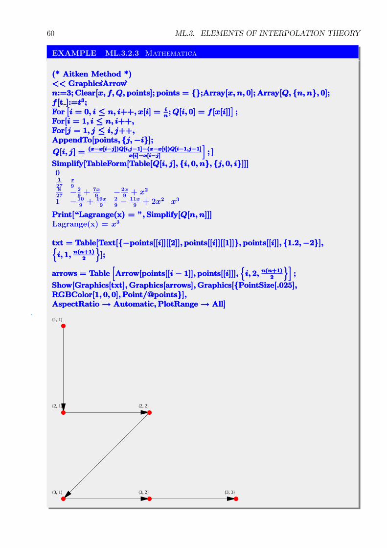
60 ML.3. ELEMENTS OF INTERPOLATION THEORY
EXAMPLE ML.3.2.3 Mathematica
(* Aitken Method *)(* Aitken Method *)(* Aitken Method *)<< GraphicsArrow<< GraphicsArrow<< GraphicsArrown:=3; Clear[x, f, Q, points]; points = {};n:=3; Clear[x, f, Q, points]; points = {};n:=3; Clear[x, f, Q, points]; points = {};Array[x, n, 0]; Array[Q, {n, n}, 0];Array[x, n, 0]; Array[Q, {n, n}, 0];Array[x, n, 0]; Array[Q, {n, n}, 0];f [t ]:=t3;f [t ]:=t3;f [t ]:=t3;For
[i = 0, i ≤ n, i++, x[i] = i
n; Q[i, 0] = f [x[i]]
];For
[i = 0, i ≤ n, i++, x[i] = i
n; Q[i, 0] = f [x[i]]
];For
[i = 0, i ≤ n, i++, x[i] = i
n; Q[i, 0] = f [x[i]]
];
For[i = 1, i ≤ n, i++,For[i = 1, i ≤ n, i++,For[i = 1, i ≤ n, i++,For[j = 1, j ≤ i, j++,For[j = 1, j ≤ i, j++,For[j = 1, j ≤ i, j++,AppendTo[points, {j, −i}];AppendTo[points, {j, −i}];AppendTo[points, {j, −i}];
Q[i, j] = (x−x[i−j])Q[i,j−1]−(x−x[i])Q[i−1,j−1]
x[i]−x[i−j]
]; ]Q[i, j] = (x−x[i−j])Q[i,j−1]−(x−x[i])Q[i−1,j−1]
x[i]−x[i−j]
]; ]Q[i, j] = (x−x[i−j])Q[i,j−1]−(x−x[i])Q[i−1,j−1]
x[i]−x[i−j]
]; ]
Simplify[TableForm[Table[Q[i, j], {i, 0, n}, {j, 0, i}]]]Simplify[TableForm[Table[Q[i, j], {i, 0, n}, {j, 0, i}]]]Simplify[TableForm[Table[Q[i, j], {i, 0, n}, {j, 0, i}]]]0127
x9
827
−29
+ 7x9
−2x9
+ x2
1 −109
+ 19x9
29
− 11x9
+ 2x2 x3
Print[“Lagrange(x) = ”, Simplify[Q[n, n]]]Print[“Lagrange(x) = ”, Simplify[Q[n, n]]]Print[“Lagrange(x) = ”, Simplify[Q[n, n]]]Lagrange(x) = x3
txt = Table[Text[{−points[[i]][[2]], points[[i]][[1]]}, points[[i]], {1.2, −2}],txt = Table[Text[{−points[[i]][[2]], points[[i]][[1]]}, points[[i]], {1.2, −2}],txt = Table[Text[{−points[[i]][[2]], points[[i]][[1]]}, points[[i]], {1.2, −2}],{i, 1, n(n+1)
2
}];
{i, 1, n(n+1)
2
}];
{i, 1, n(n+1)
2
}];
arrows = Table[Arrow[points[[i − 1]], points[[i]]],
{i, 2, n(n+1)
2
}];arrows = Table
[Arrow[points[[i − 1]], points[[i]]],
{i, 2, n(n+1)
2
}];arrows = Table
[Arrow[points[[i − 1]], points[[i]]],
{i, 2, n(n+1)
2
}];
Show[Graphics[txt], Graphics[arrows], Graphics[{PointSize[.025],Show[Graphics[txt], Graphics[arrows], Graphics[{PointSize[.025],Show[Graphics[txt], Graphics[arrows], Graphics[{PointSize[.025],RGBColor[1, 0, 0], Point/@points}],RGBColor[1, 0, 0], Point/@points}],RGBColor[1, 0, 0], Point/@points}],AspectRatio → Automatic, PlotRange → All]AspectRatio → Automatic, PlotRange → All]AspectRatio → Automatic, PlotRange → All]
1, 1
2, 1 2, 2
3, 1 3, 2 3, 3
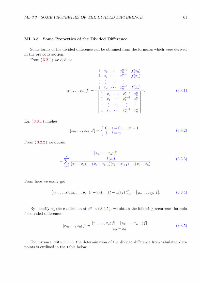
ML.3.3. SOME PROPERTIES OF THE DIVIDED DIFFERENCE 61
ML.3.3 Some Properties of the Divided Difference
Some forms of the divided difference can be obtained from the formulas which were derivedin the previous section.
From ( 3.2.1 ) we deduce
[x0, . . . , xn; f ] =
∣∣∣∣∣∣∣∣∣
1 x0 ∙ ∙ ∙ xn−10 f(x0)
1 x1 ∙ ∙ ∙ xn−11 f(x1)
......
. . ....
...1 xn ∙ ∙ ∙ xn−1
n f(xn)
∣∣∣∣∣∣∣∣∣
∣∣∣∣∣∣∣∣∣
1 x0 ∙ ∙ ∙ xn−10 xn
0
1 x1 ∙ ∙ ∙ xn−11 xn
1...
.... . .
......
1 xn ∙ ∙ ∙ xn−1n xn
n
∣∣∣∣∣∣∣∣∣
. (3.3.1)
Eq. ( 3.3.1 ) implies
[x0, . . . , xn; xi] =
{0, i = 0, . . . , n − 1;1, i = n.
(3.3.2)
From ( 3.2.2 ) we obtain
[x0, . . . , xn; f ]
=n∑
i=0
f(xi)
(xi − x0) . . . (xi − xi−1)(xi − xi+1) . . . (xi − xn).
(3.3.3)
From here we easily get
[x0, . . . , xi, y0, . . . , yj ; (t− x0) . . . (t− xi) f(t)]t = [y0, . . . , yj ; f ]. (3.3.4)
By identifying the coefficients at xn in ( 3.2.5 ), we obtain the following recurrence formulafor divided differences
[x0, . . . , xn; f ] =[x1, . . . , xn; f ]− [x0, . . . , xn−1; f ]
xn − x0
. (3.3.5)
For instance, with n = 3, the determination of the divided difference from tabulated datapoints is outlined in the table below:
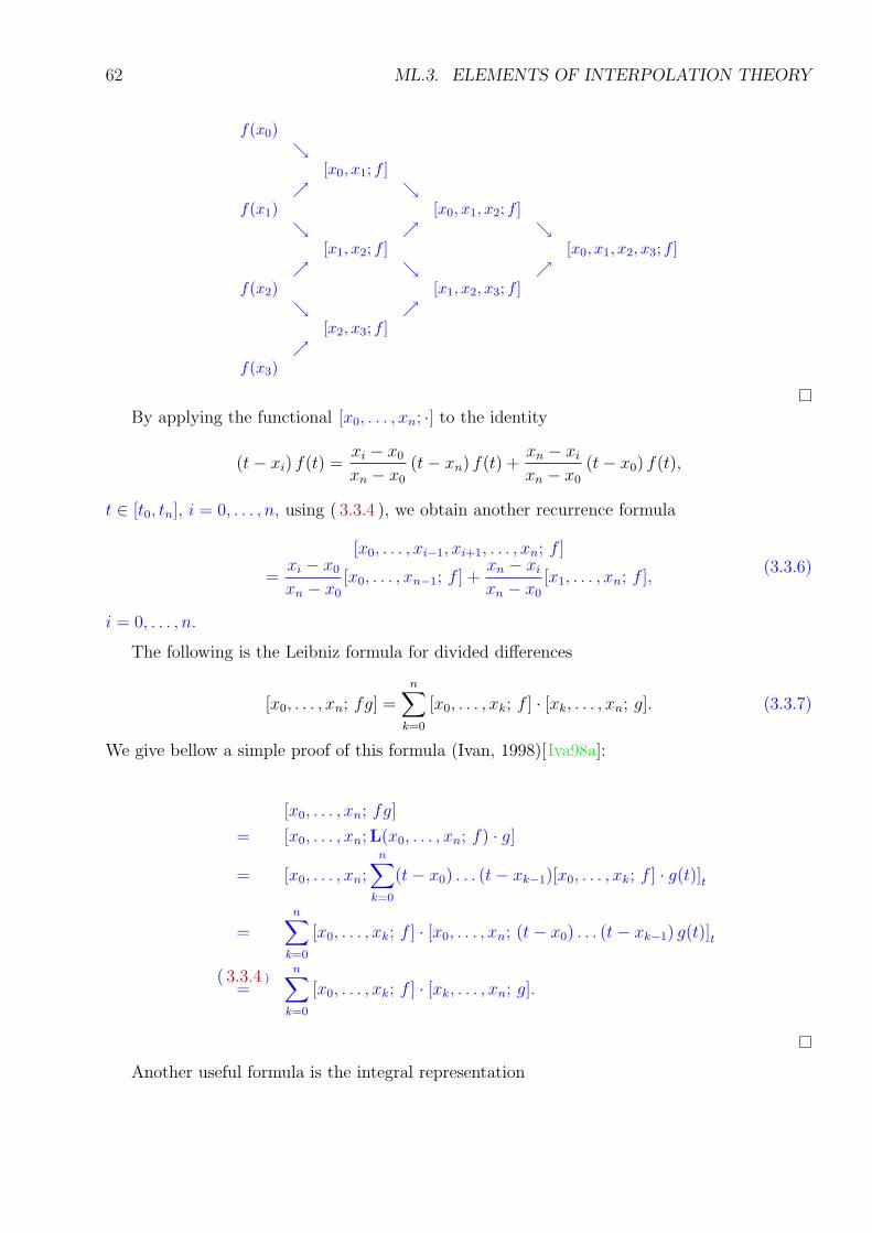
62 ML.3. ELEMENTS OF INTERPOLATION THEORY
f(x0)↘
[x0, x1; f ]↗ ↘
f(x1) [x0, x1, x2; f ]↘ ↗ ↘
[x1, x2; f ] [x0, x1, x2, x3; f ]↗ ↘ ↗
f(x2) [x1, x2, x3; f ]↘ ↗
[x2, x3; f ]↗
f(x3)
By applying the functional [x0, . . . , xn; ∙] to the identity
(t− xi) f(t) =xi − x0
xn − x0
(t− xn) f(t) +xn − xi
xn − x0
(t− x0) f(t),
t ∈ [t0, tn], i = 0, . . . , n, using ( 3.3.4 ), we obtain another recurrence formula
[x0, . . . , xi−1, xi+1, . . . , xn; f ]
=xi − x0
xn − x0
[x0, . . . , xn−1; f ] +xn − xi
xn − x0
[x1, . . . , xn; f ],(3.3.6)
i = 0, . . . , n.
The following is the Leibniz formula for divided differences
[x0, . . . , xn; fg] =n∑
k=0
[x0, . . . , xk; f ] ∙ [xk, . . . , xn; g]. (3.3.7)
We give bellow a simple proof of this formula (Ivan, 1998)[Iva98a]:
[x0, . . . , xn; fg]
= [x0, . . . , xn;L(x0, . . . , xn; f) ∙ g]
= [x0, . . . , xn;n∑
k=0
(t− x0) . . . (t− xk−1)[x0, . . . , xk; f ] ∙ g(t)]t
=n∑
k=0
[x0, . . . , xk; f ] ∙ [x0, . . . , xn; (t− x0) . . . (t− xk−1) g(t)]t
( 3.3.4 )=
n∑
k=0
[x0, . . . , xk; f ] ∙ [xk, . . . , xn; g].
Another useful formula is the integral representation
ML.3.4. MEAN VALUE PROPERTIES IN LAGRANGE INTERPOLATION 63
[x0, . . . , xk; f ]
=
1∫
0
dt1
t1∫
0
dt2 ∙ ∙ ∙
tn−1∫
0
f (n)(x0 + (x1 − x0)t1 + ∙ ∙ ∙ + (xn − xn−1)tn)dtn(3.3.8)
which is valid if f (n−1) is absolutely continuous. This can be proved by mathematical inductionon n.
If A : C[a, b] → R is a continuous linear functional which is orthogonal to all polynomialsP of degree ≤ n− 1, i.e., A(P ) = 0, then the following Peano-type representation is valid
A(f) =
∫ b
a
f (n)(t) A
((∙ − t)n−1
+
(n− 1)!
)
dt, (3.3.9)
for all f ∈ Cn[a, b], where u+ := 0 if u < 0 and u+ := u if u ≥ 0. This can be proved byapplying the functional A to both sides of the Taylor formula
f(x) = f(a) +x− a
1!f ′(a) + ∙ ∙ ∙ +
(x− a)n−1
(n− 1)!f (n−1)(a)
+1
(n− 1)!
∫ b
a
f (n)(t) (x− t)n−1+ dt.
The functional [x0, . . . , xn; ∙] is continuous on C[a, b]. Hence it has a Peano representation
[x0, . . . , xn; f ] =1
n!
∫ b
a
n ∙ [x0, . . . , xn; (∙ − t)n−1+ ] f (n)(t) dt, (3.3.10)
k = 1, . . . , n. We would like to emphasize that the Peano kernel n ∙ [x0, . . . , xn; (∙ − t)n−1+ ], a
B-spline function, is non-negative (see Remark ( ML.3.11.1 )).
If the points x0, . . . , xn are inside the simple closed curve C and f is analytic on and insideC, then
[x0, . . . , xn; f ] =1
2πi
∫
C
f(z) dz
(z − x0) . . . (z − xn). (3.3.11)
ML.3.4 Mean Value Properties in Lagrange Interpolation
Let x0, . . . , xn be a set of distinct points in the interval [a, b]. The following mean valuetheorem gives a bound for the error arising in the Lagrange interpolating-approximating process.
64 ML.3. ELEMENTS OF INTERPOLATION THEORY
THEOREM ML.3.4.1
(Lagrange Error Formula) If the function f : [a, b] → R is continuous andpossesses an (n + 1)th derivative on the interval (a, b), then for each x ∈ [a, b]there exists a point ξ(x) ∈ (a, b), such that
f(x) − L(x0, . . . , xn; f)(x) = (x − x0) . . . (x − xn)f (n+1)(ξ(x))
(n + 1)!.
Proof. If x ∈ {x0, . . . , xn} then the formula is satisfied for all ξ ∈ (a, b). Assume thatx ∈ [a, b] \ {x0, . . . , xn}. Define an auxiliary function H : [a, b]→ R, such that
H(t) = (f(t)− L(x0, . . . , xn; f)(t))(x− x0) . . . (x− xn)
− (f(x)− L(x0, . . . , xn; f)(x))(t− x0) . . . (t− xn).
Note that the function H has n + 2 roots, namely x, x0, . . . , xn. By the Generalized RolleTheorem there exists a point ξ(x) ∈ (a, b) with
H(n+1)(ξ(x)) = 0,
i.e.,
f(x)− L(x0, . . . , xn; f)(x) = (x− x0)(x− x1) . . . (x− xn)f (n+1)(ξ(x))
(n + 1)!.
The error formula given in Theorem ( ML.3.4.1 ) is an important theoretical result becauseLagrange polynomials are extremely used for deriving numerical differentiation and integrationmethods.
The well known Lagrange’s Mean Value Theorem states that if f ∈ C[x0, x1] and f ′ existson (x0, x1), then [x0, x1; f ] = f ′(ξ) for some ξ ∈ (x0, x1). This result can be generalized by thefollowing theorem.
THEOREM ML.3.4.2
If the function f : [a, b] → R is continuous and has an nth derivative on (a, b),then there exists a point ξ ∈ (a, b) such that
[x0, . . . , xn; f ] =f (n)(ξ)
n!.
Proof. Define an auxiliary function F : [a, b]→ R, such that
F (x) =
∣∣∣∣∣∣∣∣∣∣∣
1 x0 ∙ ∙ ∙ xn0 f(x0)
1 x1 ∙ ∙ ∙ xn1 f(x1)
......
. . ....
...1 xn ∙ ∙ ∙ xn
n f(xn)1 x ∙ ∙ ∙ xn f(x)
∣∣∣∣∣∣∣∣∣∣∣
.
ML.3.5. APPROXIMATION BY INTERPOLATION 65
Note that the function F has the roots x0, . . . , xn. By the Generalized Rolle Theorem, thereexists a point ξ ∈ (a, b) with
F (n)(ξ) = 0,
i.e., ∣∣∣∣∣∣∣∣∣∣∣
1 x0 ∙ ∙ ∙ xn0 f(x0)
1 x1 ∙ ∙ ∙ xn1 f(x1)
......
. . ....
...1 xn ∙ ∙ ∙ xn
n f(xn)0 0 ∙ ∙ ∙ n! f (n)(ξ)
∣∣∣∣∣∣∣∣∣∣∣
= 0.
By expanding the determinant in terms of the last row we obtain
f (n)(ξ)V (x0, . . . , xn)− n!
∣∣∣∣∣∣∣∣∣
1 x0 ∙ ∙ ∙ xn−10 f(x0)
1 x1 ∙ ∙ ∙ xn−11 f(x1)
......
. . ....
...1 xn ∙ ∙ ∙ xn−1
n f(xn)
∣∣∣∣∣∣∣∣∣
= 0
and the theorem is proved.
ML.3.5 Approximation by Interpolation
Let f ∈ C∞[a, b] be a function possessing uniform bounded derivatives.
THEOREM ML.3.5.1
If (xn)n≥0 is a sequence of distinct points in the interval [a, b], then the sequenceof Lagrange Polynomials (L(x0, . . . , xn; f))n≥0 converges uniformly to f on [a, b].
Proof. Since f has uniform bounded derivatives, then there exists a constant M > 0 suchthat |f (n)(x)| ≤ M, for all x ∈ [a, b] and n ∈ N. Let x ∈ [a, b]. By Theorem ( ML.3.4.1 ) thereexists a point ξ ∈ (a, b), such that
|f(x)− L(x0, . . . , xn; f)(x)| = |(x− x0) . . . (x− xn)||f (n+1)(ξ)|(n + 1)!
≤(b− a)n+1
(n + 1)!M.
By using
limn→∞
(b− a)n
n!= 0,
it follows that the sequence (L(x0, . . . , xn; f))n∈N converges uniformly to f on [a, b].
ML.3.6 Hermite-Lagrange Interpolating Polynomial
Let m,n ∈ N, and α0, . . . , αn ∈ N∗ such that
α0 + ∙ ∙ ∙ + αn = m + 1.
66 ML.3. ELEMENTS OF INTERPOLATION THEORY
Consider the numbers yji , i = 0, . . . , n; j = 0, . . . , αi − 1, and the distinct points x0, . . . , xn.
Then there exists a unique polynomial Hm of degree at most m, called the Hermite-Lagrangeinterpolating polynomial, such that
H(j)m (xi) = yj
i ,
for i = 0, . . . , n; j = 0, . . . , αi − 1. Define
`(x) := (x− x0)α0 . . . (x− xn)αn .
The Hermite-Lagrange interpolating polynomial can be written in the form
Hm(x) =n∑
i=0
αi−1∑
j=0
αi−j−1∑
k=0
yji
1
k!j!
((x− xi)
αi
`(x)
)(k)
x=xi
`(x)
(x− xi)αi−j−k. (3.6.1)
Let lj denotes the jth Lagrange fundamental polynomial,
lj(x) =n∏
i=1i 6=j
x− xi
xj − xi
.
THEOREM ML.3.6.1
If f ∈ C1[a, b], then the unique polynomial of least degree agreeing with f andf ′ at x0, . . . , xn is the polynomial of degree at most 2n + 1 given by
H2n+1(x) =n∑
j=0
f(xj)hj(x) +n∑
j=0
f ′(xj)gj(x),
wherehj(x) = 1 − 2(x − xj) l′j(xj) l2j (x),
gj(x) = (x − xj) l2j (x).
Proof. Since lj(xi) = δij , 0 ≤ i, j ≤ n, one can easily show that
hj(xj) = δij ,gj(xi) = 0, 0 ≤ i, j ≤ n
andh′
j(xi) = 0,g′
j(xi) = δij , 0 ≤ i, j ≤ n
ConsequentlyH2n+1(xi) = f(xi),H ′
2n+1(xi) = f ′(xi), i = 0, . . . , n.
ML.3.6. HERMITE-LAGRANGE INTERPOLATING POLYNOMIAL 67
REMARK ML.3.6.2
The divided difference for coalescing points
[ x0, . . . , x0︸ ︷︷ ︸α0−times
, . . . , xn, . . . , xn︸ ︷︷ ︸αn−times
; f ]
is defined by Tiberiu Popoviciu [Pop59] to be the coefficient at xm of theHermite-Lagrange polynomial satisfying
H(j)m (xi) = f (j)(xi),
for i = 0, . . . , n; j = 0, . . . , αi − 1.
EXAMPLE ML.3.6.3 Mathematica
(* Hermite - Lagrange *)(* Hermite - Lagrange *)(* Hermite - Lagrange *)(* InterpolatingPolynomial[data, var](* InterpolatingPolynomial[data, var](* InterpolatingPolynomial[data, var]gives a polynomial in the variable var whichgives a polynomial in the variable var whichgives a polynomial in the variable var whichprovides an exact fit to a list of data. *)provides an exact fit to a list of data. *)provides an exact fit to a list of data. *)(* The number of knots = n + 1 *)(* The number of knots = n + 1 *)(* The number of knots = n + 1 *)n = 0; Print[“Number of knots = ”, n + 1]n = 0; Print[“Number of knots = ”, n + 1]n = 0; Print[“Number of knots = ”, n + 1]Number of knots = 1(* Multiplicity of knots *)(* Multiplicity of knots *)(* Multiplicity of knots *)α0 = 2; (*α1 = 1; *)α0 = 2; (*α1 = 1; *)α0 = 2; (*α1 = 1; *)Table [αi, {i, 0, n}]Table [αi, {i, 0, n}]Table [αi, {i, 0, n}]{2}(*The degree of the Hermite − Lagrange polynomial = m *)(*The degree of the Hermite − Lagrange polynomial = m *)(*The degree of the Hermite − Lagrange polynomial = m *)m =
∑nj=0 αj − 1m =
∑nj=0 αj − 1m =
∑nj=0 αj − 1
1data =data =data =Table[Table[Table[{xi, Table [ D[f [t], {t, j}], {j, 0, αi − 1}] /. {t → xi}} , {i, 0, n}]{xi, Table [ D[f [t], {t, j}], {j, 0, αi − 1}] /. {t → xi}} , {i, 0, n}]{xi, Table [ D[f [t], {t, j}], {j, 0, αi − 1}] /. {t → xi}} , {i, 0, n}]{{x0, {f [x0] , f ′ [x0]}}}%//TableForm%//TableForm%//TableForm
x0f [x0]f ′ [x0]
H[x ] = InterpolatingPolynomial[data, x]//FullSimplifyH[x ] = InterpolatingPolynomial[data, x]//FullSimplifyH[x ] = InterpolatingPolynomial[data, x]//FullSimplifyf [x0] + (x − x0) f ′ [x0](*The divided difference on multiple knots [x0, ..., xn; f ] *)(*The divided difference on multiple knots [x0, ..., xn; f ] *)(*The divided difference on multiple knots [x0, ..., xn; f ] *)Coefficient [H[x], xm] //SimplifyCoefficient [H[x], xm] //SimplifyCoefficient [H[x], xm] //Simplifyf ′ [x0]
68 ML.3. ELEMENTS OF INTERPOLATION THEORY
ML.3.7 Finite Differences
Let F = {f | f : R→ R} and h > 0. Define the following operators:
• the identity operator, 1 : F → F ,
1 f(x) = f(x);
• the translation, displacement, or shift operator, T : F → F ,
Tf(x) = f(x + h),
introduced by George Boole [Boo60];
• the backward difference operator, ∇ : F → F ,
∇f(x) = f(x)− f(x− h);
• the forward difference operator, Δ : F → F ,
Δf(x) = f(x + h)− f(x);
• the centered difference operator, δ : F → F ,
δf(x) = f
(
x +h
2
)
− f
(
x−h
2
)
.
Some properties of the forward difference operator Δ will be presented.Since
Δ = T− 1,
the following relation can be derived
Δn = (T− 1)n,
and hence
Δnf(x) =n∑
k=0
(−1)k
(n
k
)
Tn−kf(x).
Moreover, using the relation Tif(x) = f(x + ih), we obtain
Δnf(x) =n∑
k=0
(−1)k
(n
k
)
f(x + (n− k)h). (3.7.1)
We also haven∑
k=0
(n
k
)
Δkf(x) = (1 + Δ)n f(x) = Tnf(x) = f(x + nh). (3.7.2)
ML.3.7. FINITE DIFFERENCES 69
EXAMPLE ML.3.7.1
For h = 1, since Δk1
x=
(−1)kk!
x(x + 1) . . . (x + k)=
(−1)kk!
xk+1, by ( 3.7.1 ), we obtain
n∑
k=0
(−1)knk
x(x + 1) . . . (x + k)=
1
x + n. (3.7.3)
By denoting yi = f(x + ih), i = 0, . . . , n, the forward finite differences can be calculatedas in the following table:
yn
yn−1 Δyn−1
yn−2 Δyn−2 Δ2yn−2
yn−3 Δyn−3 Δ2yn−3 Δ3yn−3
∙ ∙ ∙ ∙ ∙ ∙ ∙ ∙ ∙ ∙ ∙ ∙ ∙ ∙ ∙
y1 Δy1 Δ2y1 Δ3y1 ∙ ∙ ∙ Δn−1y1
y0 Δy0 Δ2y0 Δ3y0 ∙ ∙ ∙ Δn−1y0 Δny0
It should be noted that the finite difference is a particular case of the divided difference. Infact, with xk = x0 + k h,
[x, x + h, . . . , x + nh; f ]
=n∑
k=0
f(xk)
(xk − x0) . . . (xk − xk−1)(xk − xk+1) . . . (xk − xn)
=n∑
k=0
(−1)n−kf(x + kh)
k!(n− k)!hn
=1
n!hn
n∑
k=0
(−1)n−k
(n
k
)
f(x + kh)
=Δnf(x)
n!hn,
hence
[x, x + h, . . . , x + nh; f ] =Δnf(x)
n!hn. (3.7.4)
The relationship between the derivative of a function and the forward finite difference ispresented in the following theorem.
70 ML.3. ELEMENTS OF INTERPOLATION THEORY
THEOREM ML.3.7.2
If the function f : R → R has an nth derivative, then for each x ∈ R there existsξ ∈ (x, x + nh), such that
Δnf(x) = hnf (n)(ξ).
This is a direct consequence of ( ML.3.4.2 ) and ( 3.7.4 ).
Let C be the set of all functions possessing a Taylor expansion at all points x ∈ R. In whatfollows, Δ is taken as the restriction of the forward finite difference operator to the set C.Consider the differentiating operator D : C → C,
Df = f ′.
From
f(x + h)− f(x) =h
1!f ′(x) +
h2
2!f ′′(x) + ∙ ∙ ∙ +
hn
n!f (n)(x) + ∙ ∙ ∙
=
(hD
1!+
(hD)2
2!+ ∙ ∙ ∙ +
(hD)n
n!+ ∙ ∙ ∙
)
f(x),
we deduceΔ = ehD − 1. (3.7.5)
Likewise, we get:∇ = 1− e−hD,
δ = 2 shhD
2.
In order to represent the operator D by the operator Δ, we use the following result
ehD = 1 + Δ,
to derive
hD = ln(1 + Δ) = Δ−Δ2
2+
Δ3
3−
Δ4
4+ ∙ ∙ ∙
Furthermore, we obtain:
h2D2 = Δ2 −Δ3 +11
12Δ4 −
5
6Δ5 + ∙ ∙ ∙
h3D3 = Δ3 −3
2Δ4 +
7
4Δ5 − ∙ ∙ ∙
Taylor’s Formula can be written in the form
f(a + h) = ehDf(a).
ML.3.8. INTERPOLATION OF FUNCTIONS OF SEVERAL VARIABLES 71
Therefore
f(a + xh) = exhDf(a) = (ehD)xf(a) = (1 + Δ)xf(a),
which known as theGregory-Newton Interpolating Formula,
f(a + xh) = (1 + xΔ +x(x− 1)
2!Δ2 +
x(x− 1)(x− 2)
3!Δ3 + ∙ ∙ ∙ )f(a),
i.e.,
f(a + xh) =∞∑
n=0
(x
n
)
Δnf(a), (3.7.6)
x ∈ R.
From ( 3.7.6 ) it follows that, for any polynomial P of degree at most n, we have
P (x + a) =n∑
k=0
(x
k
)
ΔkP (a),
hence, for all x ∈ R and m ∈ Z, we obtain
P (x + m) =n∑
k=0
k∑
i=0
(x
k
)(k
i
)
(−1)k−iP (m + i). (3.7.7)
PROBLEM ML.3.7.3
Let P be a polynomial of degree at most n with real coefficients. Suppose thatP takes integer values at some n + 1 consecutive integers. Prove that P takesinteger values at any integer number.
We simply use representation ( 3.7.7 ) for P .
ML.3.8 Interpolation of Functions of Several Variables
Let a ≤ x0 < ∙ ∙ ∙ < xn ≤ b and c ≤ y0 < ∙ ∙ ∙ < ym ≤ d. Define
F = {f | f : [a, b]× [c, d]→ R},
and
ui : [a, b]→ R, vj : [c, d]→ R
be functions satisfying the conditions:
ui(xk) = δik, i, k = 0, . . . , n;
vj(yh) = δjh, j, h = 0, . . . ,m.
72 ML.3. ELEMENTS OF INTERPOLATION THEORY
Define the interpolating operators U, V : F → F , by
Uf(x, y) =n∑
i=0
f(xi, y)ui(x),
V f(x, y) =m∑
j=0
f(x, yj)vj(y).
Note that:
Uf(xk, y) = f(xk, y) and V f(x, yh) = f(x, yh),
k = 0, . . . , n; h = 0, . . . ,m; x ∈ [a, b], y ∈ [c, d].
DEFINITION ML.3.8.1
The operator UV is called the tensor product of the operators U and V.
Note that we have
UV f(x, y) =n∑
i=0
m∑
j=0
f(xi, yj) ui(x) vj(y)
and
UV f(xk, yh) = f(xk, yh),
k = 0, . . . , n; h = 0, . . . ,m.
DEFINITION ML.3.8.2
The operator U ⊕ V := U + V − UV is called the Boolean sum of the operatorsU and V.
Note that:
U ⊕ V f(xk, y) = f(xk, y), U ⊕ V f(x, yh) = f(x, yh),
k = 0, . . . , n; h = 0, . . . ,m; x ∈ [a, b], y ∈ [c, d].
ML.3.9 Scattered Data Interpolation. Shepard’s Method
In many fields such as geology, meteorology and cartography, we frequently encounternonuniformly spaced data, also called scattered data, which have to be interpolated.
The interpolation problem can be stated as follows. Suppose that a set of n distinct abscissaeXi = (xi, yi) ∈ R2, and the associated ordinates zi, i = 1, . . . , n, are given. Then we seek afunction f : R2 → R such that f(Xi) = zi, i = 1, . . . , n.
In a global method, the interpolant depends on all the data points at once in the sense thatadding, changing, or removing one data point implies that we have to solve the problem again.
In a local method, adding, changing or removing a data point affects the interpolant onlylocally, i.e., in a certain subset of the domain.
ML.3.9. SCATTERED DATA INTERPOLATION. SHEPARD’S METHOD 73
The Shepard interpolant to the data (Xi; zi) ∈ R3, i = 1, . . . , n, is a weighted mean of theordinates zi :
S(X) :=n∑
i=1
ωi(X) zi, X ∈ R3, (3.9.1)
with weight functions
ωi(X) :=
n∏
j=1j 6=i
ρμi(X,Xj)
n∑
k=1
n∏
j=1j 6=k
ρμi(X,Xj)
where ρ is a metric on R2 and μi > 0. For X 6= Xi, i = 1, . . . , n, we can write
ωi(X) =
1
ρμi(X,Xi)n∑
k=1
1
ρμi(X,Xk)
, i = 1, . . . , n.
This is a kind of inverse distance weighted method, i.e., the larger the distance of X to Xi,the less influence zi has on the value of S at the point X.
Now, we assume that ρ is the Euclidean metric on R2. The functions ωi have the followingproperties:
• ωi ∈ C0, continuity;
• ωi(X) ≥ 0, positivity;
• ωi(Xj) = δij , interpolation property (S(Xi) = zi);
•n∑
i=1
ωi(X) = 1, normalization.
It can be shown that the Shepard interpolant ( 3.9.1 ) has
• cusps at Xi if 0 < μi < 1,
• corners at Xi if μi = 1,
• flat spots at Xi if μi > 1, i.e., the tangent planes at such points are parallel to the (x, y)plane.
Besides the obvious weaknesses of Shepard’s method, clearly all of the functions ωi(X) haveto be recomputed as soon as just one data point is changed, or a data point is added or removed.This shows that Shepard’s method is a global method.
There are several ways to improve Shepard’s method, for example by removing the dis-continuities in the derivatives and the flat spots at the interpolation points. Even the globalcharacter can be made local using the following procedures:
74 ML.3. ELEMENTS OF INTERPOLATION THEORY
1. multiply the weight functions ωi by a mollifying function λi :
λi(Xi) = 1,
λi(X) ≥ 0, inside a given neighborhood Bi of Xi,
λi(X) = 0, outside of Bi,
2. use weight functions which are locally supported like B-splines,
3. use a recurrence formula. Consider the weight functions
ek(X) :=
k−1∏
j=1
ρμ(X,Xj)
k∑
j=1
k∏
i=1i 6=j
ρμ(X,Xi)
, k = 2, . . . n,
and the recurrence formula
s1(X) = z1,sk(X) = sk−1(X) + ek(X)(zk − sk−1(Xk)), k = 2, . . . , n.
(3.9.2)
We have obtained a recursive formula for the Shepard-type interpolant sn.
ML.3.10 Splines
Splines are piecewise polynomials with R as their natural domain of definition. They oftenappear as solutions to extremal problems. Splines also appears as kernels of interpolationsformulas. The systematic study of splines has begun with the work of Isaac Jacob Schoenbergin the forties.
We would like to emphasize that it is Tiberiu Popoviciu who defined the so called “ele-mentary functions of order n”, later referred as splines. Results of Popoviciu’s work were alsoknown by I. J. Schoenberg (see M. Mardens and I. J. Schoenberg, On the variation diminishingspline approximation methods, Mathematica 8(31),1, 1966, pp. 61–82 (dedicated to TiberiuPopoviciu on his 60th birthday)).
At present, splines are widely used in numerical computation and are indispensable for manytheoretical questions.
A typical spline is the truncated power
(x− a)k+ :=
{0, if x < a,
(x− a)k, if x ≥ a,
where k ∈ N∗. With k = 0, we obtain the Heaviside function
(x− a)0+ :=
{0, if x < a,1, if x ≥ a,
Let n, p ∈ N∗ and (a = x0 < ∙ ∙ ∙ < xn = b) be a division of the interval [a, b].
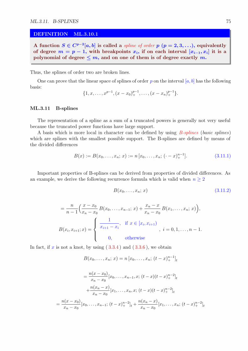
ML.3.11. B-SPLINES 75
DEFINITION ML.3.10.1
A function S ∈ Cp−2[a, b] is called a spline of order p (p = 2, 3, . . .), equivalentlyof degree m = p − 1, with breakpoints xi, if on each interval [xi−1, xi] it is apolynomial of degree ≤ m, and on one of them is of degree exactly m.
Thus, the splines of order two are broken lines.
One can prove that the linear space of splines of order p on the interval [a, b] has the followingbasis:
{1, x, . . . , xp−1, (x− x0)p−1+ , . . . , (x− xn)p−1
+ }.
ML.3.11 B-splines
The representation of a spline as a sum of a truncated powers is generally not very usefulbecause the truncated power functions have large support.
A basis which is more local in character can be defined by using B-splines (basic splines)which are splines with the smallest possible support. The B-splines are defined by means ofthe divided differences
B(x) := B(x0, . . . , xn; x) := n [x0, . . . , xn; (∙ − x)n−1+ ]. (3.11.1)
Important properties of B-splines can be derived from properties of divided differences. Asan example, we derive the following recurrence formula which is valid when n ≥ 2
B(x0, . . . , xn; x) (3.11.2)
=n
n− 1
( x− x0
xn − x0
B(x0, . . . , xn−1; x) +xn − x
xn − x0
B(x1, . . . , xn; x)),
B(xi, xi+1; x) =
1
xi+1 − xi
, if x ∈ [xi, xi+1)
0, otherwise
, i = 0, 1, . . . , n − 1.
In fact, if x is not a knot, by using ( 3.3.4 ) and ( 3.3.6 ), we obtain
B(x0, . . . , xn; x) = n [x0, . . . , xn; (t− x)n−1+ ]t
=n(x− x0)xn − x0
[x0, . . . , xn−1, x; (t− x)(t− x)n−2+ ]t
+n(xn − x)xn − x0
[x1, . . . , xn, x; (t− x)(t− x)n−2+ ]t
=n(x− x0)xn − x0
[x0, . . . , xn−1; (t− x)n−2+ ]t +
n(xn − x)xn − x0
[x1, . . . , xn; (t− x)n−2+ ]t
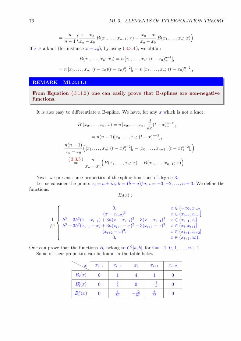
76 ML.3. ELEMENTS OF INTERPOLATION THEORY
=n
n− 1
( x− x0
xn − x0
B(x0, . . . , xn−1; x) +xn − x
xn − x0
B(x1, . . . , xn; x)).
If x is a knot (for instance x = x0), by using ( 3.3.4 ), we obtain
B(x0, . . . , xn; x0) = n [x0, . . . , xn; (t− x0)n−1+ ]t
= n [x0, . . . , xn; (t− x0)(t− x0)n−2+ ]t = n [x1, . . . , xn; (t− x0)
n−2+ ]t.
REMARK ML.3.11.1
From Equation ( 3.11.2 ) one can easily prove that B-splines are non-negativefunctions.
It is also easy to differentiate a B-spline. We have, for any x which is not a knot,
B′(x0, . . . , xn; x) = n [x0, . . . , xn;d
dx(t− x)n−1
+ ]t
= n(n− 1)[x0, . . . , xn; (t− x)n−2+ ]t
=n(n− 1)
xn − x0
([x1, . . . , xn; (t− x)n−2
+ ]t − [x0, . . . , xn−1; (t− x)n−2+ ]t
)
( 3.3.5 )=
n
xn − x0
(B(x1, . . . , xn; x)− B(x0, . . . , xn−1; x)
).
Next, we present some properties of the spline functions of degree 3.Let us consider the points xi = a + ih, h = (b− a)/n, i = −3,−2, . . . , n + 3. We define the
functions:Bi(x) :=
1
h3
0, x ∈ (−∞, xi−2](x− xi−2)
3 x ∈ (xi−2, xi−1]h3 + 3h2(x− xi−1) + 3h(x− xi−1)
2 − 3(x− xi−1)3, x ∈ (xi−1, xi]
h3 + 3h2(xi+1 − x) + 3h(xi+1 − x)2 − 3(xi+1 − x)3, x ∈ (xi, xi+1](xi+2 − x)3, x ∈ (xi+1, xi+2]
0, x ∈ (xi+2,∞).
One can prove that the functions Bi belong to C2[a, b], for i = −1, 0, 1, . . ., n + 1.Some of their properties can be found in the table below.
HHHHHx xi−2 xi−1 xi xi+1 xi+2
01410Bi(x)
B′i(x) 0 3
h 0 − 3h 0
06h2− 12
h26h20B′′
i (x)
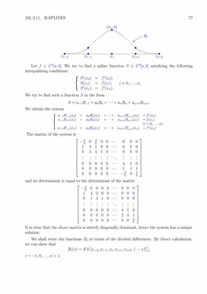
ML.3.11. B-SPLINES 77
• • • • •
••
•
xi−2 xi−1 xi xi+1 xi+2
(xi, 4)
Bi���+
Let f ∈ C1[a, b]. We try to find a spline function S ∈ C2[a, b] satisfying the followinginterpolating conditions:
S ′(x0) = f ′(x0),S(xi) = f(xi), i = 0, . . . , n,S ′(xn) = f ′(xn).
We try to find such a function S in the form
S = a−1B−1 + a0B0 + ∙ ∙ ∙ + anBn + an+1Bn+1.
We obtain the system
a−1B′−1(x0) + a0B
′0(x0) + ∙ ∙ ∙+ an+1B
′n+1(x0) = f ′(x0)
a−1B−1(xi) + a0B0(xi) + ∙ ∙ ∙+ an+1Bn+1(xi) = f(xi)(i = 0, . . . , n)
a−1B′−1(xn) + a0B
′0(xn) + ∙ ∙ ∙+ an+1B
′n+1(xn) = f ′(xn)
The matrix of the system is
− 3h
0 3h
0 0 ∙ ∙ ∙ 0 0 01 4 1 0 0 ∙ ∙ ∙ 0 0 00 1 4 1 0 ∙ ∙ ∙ 0 0 0...
......
......
. . ....
......
0 0 0 0 0 ∙ ∙ ∙ 4 1 00 0 0 0 0 ∙ ∙ ∙ 1 4 10 0 0 0 0 ∙ ∙ ∙ − 3
h0 3
h
and its determinant is equal to the determinant of the matrix
− 3h
0 0 0 0 ∙ ∙ ∙ 0 0 01 4 2 0 0 ∙ ∙ ∙ 0 0 00 1 4 1 0 ∙ ∙ ∙ 0 0 0...
......
......
. . ....
......
0 0 0 0 0 ∙ ∙ ∙ 4 1 00 0 0 0 0 ∙ ∙ ∙ 2 4 10 0 0 0 0 ∙ ∙ ∙ 0 0 3
h
.
It is clear that the above matrix is strictly diagonally dominant, hence the system has a uniquesolution.
We shall write the functions Bi in terms of the divided differences. By direct calculation,we can show that
Bi(x) = 4! h [xi−2, xi−1, xi, xi+1, xi+2; (∙ − x)3+],
i = −1, 0, . . . , n + 1.
78 ML.3. ELEMENTS OF INTERPOLATION THEORY
ML.3.12 Problems
Let x0, . . . , xn be distinct points on the real axis, f be a function defined on these pointsand `(x) = (x− x0) . . . (x− xn).
PROBLEM ML.3.12.1
Let P be a polynomial. Prove that the Lagrange Polynomial L(x0, . . . , xn; P )is the remainder obtained by dividing the polynomial P by the polynomial(X − x0) . . . (X − xn).
Let P (x) = Q(x) (x − x0) . . . (x − xn) + R(x). We have R(xi) = P (xi) for i = 0, . . . , n. Sincethe degree of the polynomial R is at most n, we get R = L(x0, . . . , xn; P ).
PROBLEM ML.3.12.2
Calculate L(x0, . . . , xn; Xn+1).
We have
Xn+1 = 1 ∙ (X − x0)(X − x1) . . . (X − xn)
+Xn+1 − (X − x0)(X − x1) . . . (X − xn).
By P. ( ML.3.12.1 ) we obtain
L(x0, . . . , xn; Xn+1) = Xn+1 − (X − x0)(X − x1) . . . (X − xn).
PROBLEM ML.3.12.3
Let Pn : R → R be a polynomial of degree at most n, n ∈ N. Prove thedecomposition in partial fractions
Pn(x)
(x − x0) . . . (x − xn)=
n∑
k=0
1
x − xi∙
P (xi)
`′(xi).
With `(x) = (x− x0) . . . (x− xn), we have
Pn(x)
`(x)=
L(x0, . . . , xn; Pn)(x)
`(x)=
n∑
k=0
1
x− xi
∙P (xi)
`′(xi).
PROBLEM ML.3.12.4
Calculate the sum
n∑
i=0
xki(xi − x0) . . . (xi − xi−1)(xi − xi+1) . . . (xi − xn)
,
k = 0, . . . , n.
ML.3.12. PROBLEMS 79
PROBLEM ML.3.12.5
Calculate[x0, . . . , xn; x
k],
for k = n, n + 1.
PROBLEM ML.3.12.6
Calculate[x0, . . . , xn; (X − x0) . . . (X − xk)],
k ∈ N.
PROBLEM ML.3.12.7
Prove that
L(x0, . . . , xn; L(x1, . . . , xn; f)) = L(x1, . . . , xn; L(x0, . . . , xn; f)).
PROBLEM ML.3.12.8
Prove that, for x /∈ {x0, . . . , xn},
[
x0, . . . , xn;f(t)
x − t
]
t
=L(x0, . . . , xn; f)(x)
(x − x0) . . . (x − xn).
With `(x) = (x− x0) . . . (x− xn), we have
L(x0, . . . , xn; f)(x) =n∑
k=0
`(x)
x− xi
∙f(xi)
`′(xi),
hence
L(x0, . . . , xn; f)(x)
`(x)=
n∑
k=0
f(xi)x−xi
`′(xi)=
[
x0, . . . , xn;f(t)
x− t
]
t
.
PROBLEM ML.3.12.9
If f(x) = 1x
and 0 < x0 < x1 < ∙ ∙ ∙ < xn, then
[x0, . . . , xn; f ] =(−1)n
x0 . . . xn.
80 ML.3. ELEMENTS OF INTERPOLATION THEORY
By using problem ( ML.3.12.8 ), we have
[
x0, . . . , xn;1
t
]
t
= −L(x0, . . . , xn; 1)(0)
(0− x0) . . . (0− xn)=
(−1)n
x0 . . . xn
.
Solution 2. We write the obvious equality
[
x0, . . . , xn;(t− t0) . . . (t− xn)
t
]
= 0
in the form[
x0, . . . , xn; tn − (t0 + ∙ ∙ ∙ + tn)tn−1 + ∙ ∙ ∙ + (−1)n+1 t0 . . . xn
t
]
= 0,
i.e.,
1− (t0 + ∙ ∙ ∙ + tn)0 + ∙ ∙ ∙ + 0 + (−1)n+1t0 . . . xn
[
x0, . . . , xn;1
t
]
= 0.
ML.4
Elements of Numerical Integration
ML.4.1 Richardson’s Extrapolation
Extrapolation is applied when it is known that the approximation technique has an errorterm with a predictable form, one that depends on a parameter, usually the step size h.
Richardson’s extrapolation is a technique frequently employed to generate results of highaccuracy by using low-order formulas.
Let 1 < p1 < p2 < . . . be a sequence of integers and F be a formula that approximates anunknown value M. Suppose that, in a neighborhood of the point zero, the following relationholds
M = F (h) + a1hp1 + a2h
p2 + ∙ ∙ ∙
where a1, a2, . . . are constants. The order of approximation for F (h) is O(hp1). By denoting
F1(h) := F (h), a11 := a1, a12 := a2, . . .
we obtainM = F1(h) + a11h
p1 + a12hp2 + ∙ ∙ ∙ .
For q > 1, we deduce
M = F1
(h
q
)
+ a11
(h
q
)p1
+ a12
(h
q
)p2
+ ∙ ∙ ∙ ,
hence, by letting
F2(h) =qp1F1
(hq
)− F1 (h)
qp1 − 1,
we obtainM = F2 (h) + 0 ∙ hp1 + a22 hp2 + ∙ ∙ ∙ ,
i.e., the formula F2(h) has order of approximation O(hp2).Step by step, we deduce approximation formulas of order O(hpj ) :
Fj(h) =qpj−1Fj−1
(hq
)− Fj−1 (h)
qpj−1 − 1, (4.1.1)
81
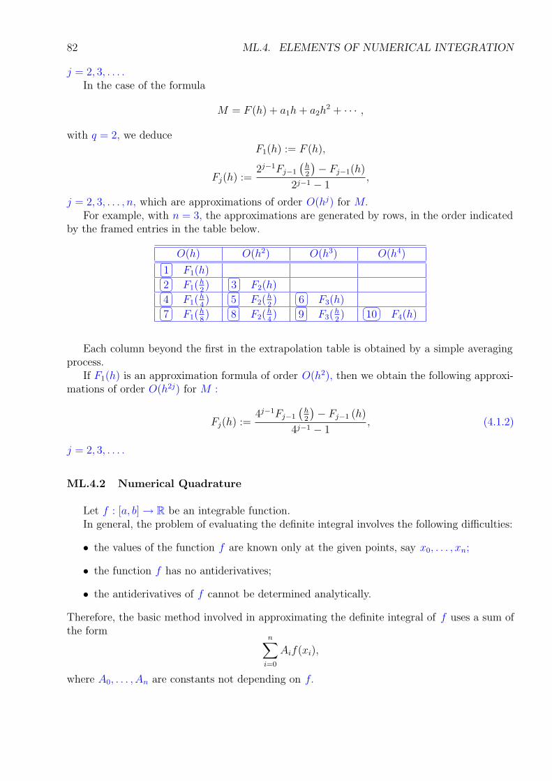
82 ML.4. ELEMENTS OF NUMERICAL INTEGRATION
j = 2, 3, . . . .In the case of the formula
M = F (h) + a1h + a2h2 + ∙ ∙ ∙ ,
with q = 2, we deduceF1(h) := F (h),
Fj(h) :=2j−1Fj−1
(h2
)− Fj−1(h)
2j−1 − 1,
j = 2, 3, . . . , n, which are approximations of order O(hj) for M.For example, with n = 3, the approximations are generated by rows, in the order indicated
by the framed entries in the table below.
O(h) O(h2) O(h3) O(h4)�
�
�
�1 F1(h)�
�
�
�2 F1(h2)�
�
�
�3 F2(h)�
�
�
�4 F1(h4)�
�
�
�5 F2(h2)�
�
�
�6 F3(h)�
�
�
�7 F1(h8)�
�
�
�8 F2(h4)�
�
�
�9 F3(h2)�
�
�
�10 F4(h)
Each column beyond the first in the extrapolation table is obtained by a simple averagingprocess.
If F1(h) is an approximation formula of order O(h2), then we obtain the following approxi-mations of order O(h2j) for M :
Fj(h) :=4j−1Fj−1
(h2
)− Fj−1 (h)
4j−1 − 1, (4.1.2)
j = 2, 3, . . . .
ML.4.2 Numerical Quadrature
Let f : [a, b]→ R be an integrable function.In general, the problem of evaluating the definite integral involves the following difficulties:
• the values of the function f are known only at the given points, say x0, . . . , xn;
• the function f has no antiderivatives;
• the antiderivatives of f cannot be determined analytically.
Therefore, the basic method involved in approximating the definite integral of f uses a sum ofthe form
n∑
i=0
Aif(xi),
where A0, . . . , An are constants not depending on f.
ML.4.3. ERROR BOUNDS IN THE QUADRATURE METHODS 83
DEFINITION ML.4.2.1
A relation of the form
∫ b
a
f(x) dx =n∑
i=0
Aif(xi) + Rn(f),
is called a quadrature formula.
The number Rn(f) is the remainder of the quadrature formula ( ML.4.2.1 ). The previousequality is sometimes written in the form
∫ b
a
f(x) dx ≈n∑
i=0
Aif(xi).
DEFINITION ML.4.2.2
The degree of accuracy, or degree of precision of the quadrature formula ( ML.4.2.1 )is the positive integer m such that
Rn(Xk) = 0, k = 0, . . . , m, Rn(X
m+1) 6= 0.
The quadrature formulas can be classified as follows:
• Newton-Cotes type, when the nodes x0, . . . , xn are given and the coefficients A0, . . . , An
are determined such that the degree of precision is at least n;
• Chebyshev type, when the coefficients A0, . . . , An are equal one to the other and thenodes x0, . . . , xn are determined such that the degree of precision is at least n;
• Gauss type, when coefficients A0, . . . , An and the nodes x0, . . . , xn, are determined suchthat the degree of precision is maximal.
ML.4.3 Error Bounds in the Quadrature Methods
Let f ∈ Cn+1[a, b]. Consider a quadrature formula
∫ b
a
f(x) dx =n∑
i=0
Aif(xi) + Rn(f)
with order of precision n. Using Taylor’s formula with integral form of the remainder
f(x) =n∑
j=0
f (j)(a)
j!(x− a)j +
1
n!
∫ x
a
(x− t)nf (n+1)(t)dt,
x ∈ [a, b], we obtainRn(f)
84 ML.4. ELEMENTS OF NUMERICAL INTEGRATION
= Rn
(n∑
j=0
f (j)(a)
j!(X − a)j
)
+1
n!Rn
(∫ X
a
(X − t)nf (n+1)(t)dt
)
=1
n!Rn
(∫ X
a
(X − t)nf (n+1)(t)dt
)
=
∫ b
a
1
n!
∫ x
a
(x− t)nf (n+1)(t)dt dx−1
n!
n∑
i=0
Ai
∫ xi
a
(xi − t)nf (n+1)(t)dt
=
∫ b
a
1
n!
∫ b
t
(x− t)nf (n+1)(t)dx dt−1
n!
n∑
i=0
Ai
∫ b
a
(xi − t)n+f (n+1)(t)dt
=
∫ b
a
((b− t)n+1
(n + 1)!−
1
n!
n∑
i=0
Ai(xi − t)n+
)
f (n+1)(t)dt.
By denoting
Kn =
∫ b
a
∣∣∣∣∣(b− t)n+1
(n + 1)!−
1
n!
n∑
i=0
Ai(xi − t)n+
∣∣∣∣∣dt,
which is a constant not depending on f and using the notation
‖f (n+1)‖ = maxa≤x≤b
|f (n+1)(x)|,
we obtain an error bound in quadrature formula:
|Rn(f)| ≤ Kn‖f(n+1)‖.
ML.4.4 Trapezoidal Rule
The idea used to produce trapezoidal rule is to approximate the function f : [a, b]→ R bythe Lagrange interpolating polynomial L(a, b; f).
THEOREM ML.4.4.1
If f ∈ C2[a, b], then there exists ξ ∈ (a, b) such that the following quadratureformula holds
∫ b
a
f(x)dx = (b − a)f(a) + f(b)
2−
(b − a)3
12f ′′(ξ).
Proof. We have∫ b
a
L(a, b; f)(x)dx
=
∫ b
a
(x− a
b− af(b) +
b− x
b− af(a)
)
dx = (b− a)f(a) + f(b)
2.
ML.4.5. RICHARDSON’S DEFERRED APPROACH TO THE LIMIT 85
By using the weighted mean value theorem, we obtain
R1(f) =
∫ b
a
(f(x)− L(a, b; f)(x))dx
=
∫ b
a
(x− a)(x− b)[a, b, x; f ]dx = [a, b, c; f ]
∫ b
a
(x− a)(x− b)dx
=f ′′(ξ)
2
∫ b
a
((x− a)2 − (x− a)(b− a)
)dx
=f ′′(ξ)
2
((x− a)3
3−
(x− a)2
2(b− a)
)∣∣∣∣
b
a
= −(b− a)3
12f ′′(ξ).
We have proved that the trapezoidal quadrature formula has degree of precision 1. To gener-alize this procedure, choose a positive integer n. Subdivide the interval [a, b] into n subintervals[xi−1, xi], xi = a+ i b−a
n, i = 0, . . . , n, and apply trapezoidal rule on each subinterval. We obtain
n∑
i=1
b− a
2n(f(xi−1) + f(xi)) =
b− a
n
(f(a) + f(b)
2+
n−1∑
i=1
f(xi)
)
and
R(f) = −n∑
i=1
(b− a)3
12n3f ′′(ξi) = −
(b− a)3
12n2
1
n
n∑
i=1
f ′′(ξi)
= −(b− a)3
12n2f ′′(ξ) = −
b− a
12h2f ′′(ξ),
where h =b− a
n. Consequently, there exists ξ ∈ (a, b) such that
∫ b
a
f(x)dx =b− a
n
(f(a) + f(b)
2+
n−1∑
i=1
f(xi)
)
−(b− a)3
12n2f ′′(ξ). (4.4.1)
This formula is known as the composite trapezoidal rule. It is one of the simplest formulas fornumerical integration.
ML.4.5 Richardson’s Deferred Approach to the Limit
Let T (h) be the result from the trapezoidal rule using step size h and T (l) be the resultwith step size l, such that h < l.
If the second derivative f ′′ is “reasonably constant”, then:
∫ b
a
f(x) dx ≈ T (h) + Ch2,
86 ML.4. ELEMENTS OF NUMERICAL INTEGRATION
∫ b
a
f(x) dx ≈ T (l) + Cl2.
We deduce
C ≈T (h)− T (l)
l2 − h2,
hence ∫ b
a
f(x) dx ≈ T (h) + h2 T (h)− T (l)
l2 − h2=
=( l
h)2T (h)− T (l)
( lh)2 − 1
.
This gives a better approximation to∫ b
af(x) dx than T (h) and T (l). In fact, if the second
derivative is actually a constant, then the truncation error is zero.
ML.4.6 Romberg Integration
Romberg Integration uses the Composite Trapezoidal Rule to give preliminary approxima-tions and then applies the Richardson Extrapolation process to improve the approximations.
Denoting by T (h) the approximation of the integral I =∫ b
af(x)dx given by the Composite
Trapezoidal rule,
T (h) =h
2
(
f(a) + f(b) + 2m−1∑
i=1
f(a + ih)
)
,
where h = (b− a)/m, it can be shown that if f ∈ C∞[a, b], the Composite Trapezoidal rule canbe written in the form ∫ b
a
f(x)dx = T (h) + a1h2 + a2h
4 + ∙ ∙ ∙ ,
therefore, we can apply Richardson Extrapolation.Let n ∈ N∗,
hk =b− a
2k−1, k = 1, . . . , n.
The following Composite Trapezoidal approximations with m = 1, 2, . . ., 2n−1, can be derived:
R1,1 = h1f(a) + f(b)
2,
Rk,1 =hk
2
f(a) + f(b) + 22k−1−1∑
i=1
f(a + ihk)
,
k = 2, . . . , n. We can rewrite Rk,1 in the form:
Rk,1 =1
2
Rk−1,1 + hk−1
2k−2∑
i=1
f(a + (2i− 1)hk)
, k = 2, . . . , n.
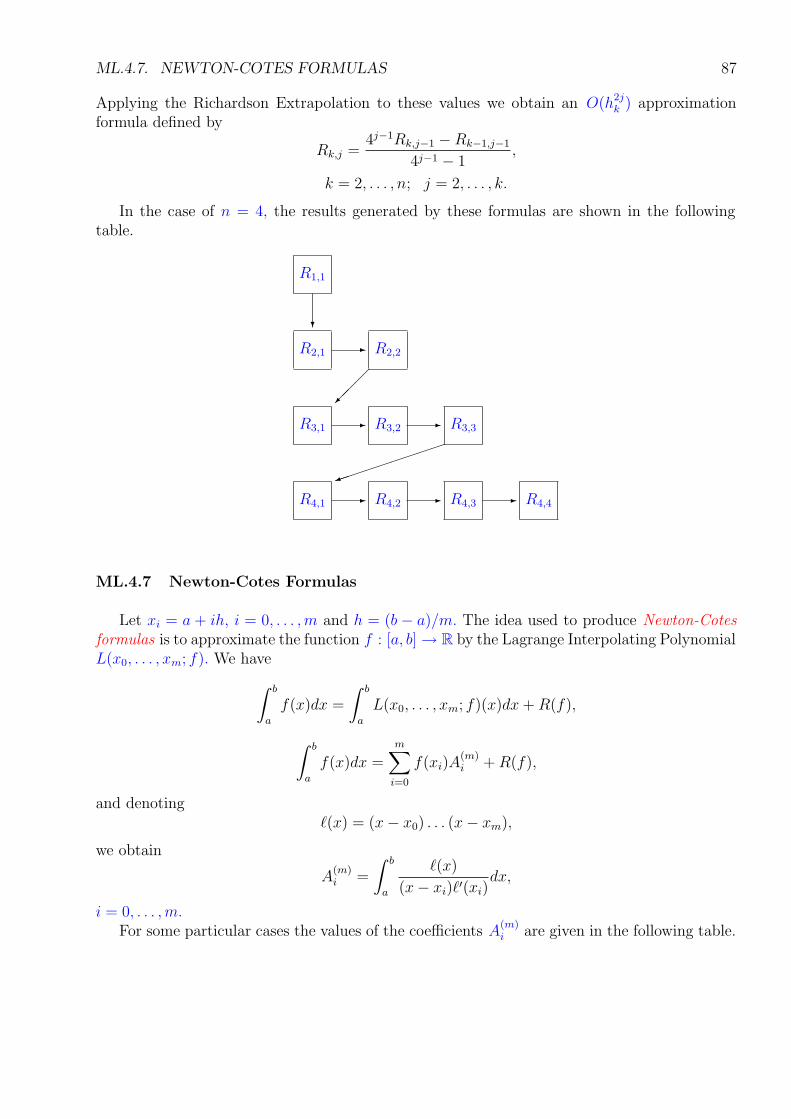
ML.4.7. NEWTON-COTES FORMULAS 87
Applying the Richardson Extrapolation to these values we obtain an O(h2jk ) approximation
formula defined by
Rk,j =4j−1Rk,j−1 − Rk−1,j−1
4j−1 − 1,
k = 2, . . . , n; j = 2, . . . , k.
In the case of n = 4, the results generated by these formulas are shown in the followingtable.
R4,1 R4,2 R4,3 R4,4
R3,1 R3,2 R3,3
R2,1 R2,2
R1,1
?
-
���
- -
���������)
- - -
ML.4.7 Newton-Cotes Formulas
Let xi = a + ih, i = 0, . . . ,m and h = (b − a)/m. The idea used to produce Newton-Cotesformulas is to approximate the function f : [a, b]→ R by the Lagrange Interpolating PolynomialL(x0, . . . , xm; f). We have
∫ b
a
f(x)dx =
∫ b
a
L(x0, . . . , xm; f)(x)dx + R(f),
∫ b
a
f(x)dx =m∑
i=0
f(xi)A(m)i + R(f),
and denoting`(x) = (x− x0) . . . (x− xm),
we obtain
A(m)i =
∫ b
a
`(x)
(x− xi)`′(xi)dx,
i = 0, . . . ,m.For some particular cases the values of the coefficients A
(m)i are given in the following table.
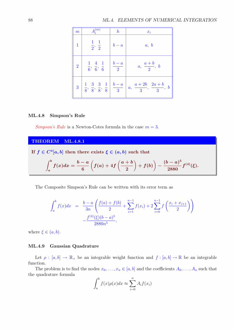
88 ML.4. ELEMENTS OF NUMERICAL INTEGRATION
m A(m)i h xi
11
2,
1
2b− a a, b
21
6,
4
6,
1
6
b− a
2a,
a + b
2, b
31
8,
3
8,
3
8,
1
8
b− a
3a,
a + 2b
3,
2a + b
3, b
ML.4.8 Simpson’s Rule
Simpson’s Rule is a Newton-Cotes formula in the case m = 3.
THEOREM ML.4.8.1
If f ∈ C4[a, b] then there exists ξ ∈ (a, b) such that
∫ b
a
f(x)dx =b − a
6
(
f(a) + 4f
(a + b
2
)
+ f(b)
)
−(b − a)5
2880f (4)(ξ).
The Composite Simpson’s Rule can be written with its error term as
∫ b
a
f(x)dx =b− a
3n
(f(a) + f(b)
2+
n−1∑
i=1
f(xi) + 2n−1∑
i=0
f
(xi + xi+1
2
))
−f (4)(ξ)(b− a)5
2880n5,
where ξ ∈ (a, b).
ML.4.9 Gaussian Quadrature
Let ρ : [a, b] → R+ be an integrable weight function and f : [a, b]→ R be an integrablefunction.
The problem is to find the nodes x0, . . . , xn ∈ [a, b] and the coefficients A0, . . . , An such thatthe quadrature formula ∫ b
a
f(x)ρ(x)dx ≈n∑
i=0
Aif(xi)
ML.4.9. GAUSSIAN QUADRATURE 89
have a maximal degree of precision.Let (ϕn)n∈N be the sequence of orthogonal polynomials associated with the weight function
ρ, where degree(ϕn) = n. Let x0, . . . , xn be the roots of the polynomial ϕn+1 and L(x0, . . . , xn; f)be the Lagrange interpolating polynomial.
THEOREM ML.4.9.1
The quadrature formula
∫ b
a
f(x)ρ(x)dx ≈n∑
i=0
Aif(xi) =
∫ b
a
L(x0, . . . , xn; f)(x)ρ(x)dx
has degree of precision 2n + 1.
Proof. Let P a polynomial of degree at most 2n + 1. We divide the polynomial P to thepolynomial ϕn+1 :
P = Qϕn+1 + r,
where degree(Q) ≤ n and degree(r) ≤ n. We have:
L(x0, . . . , xn; P ) = L(x0, . . . , xn; Qϕn+1)︸ ︷︷ ︸0
+L(x0, . . . , xn; r) = r,
R(P ) =
∫ b
a
(P (x)− L(x0, . . . , xn; P )(x))ρ(x)dx
=
∫ b
a
(P (x)− r(x))ρ(x)dx
=
∫ b
a
Q(x)ϕn+1(x)ρ(x)dx = 0.
It follows that the degree of precision is at least 2n + 1.On the other hand, from the equalities
R(ϕ2n+1) =
∫ b
a
(ϕ2n+1(x)− L(x0, . . . , xn; ϕ2
n+1)(x))︸ ︷︷ ︸
0
ρ(x)dx
=
∫ b
a
ϕ2n+1(x)ρ(x)dx > 0,
we deduce that it cannot be greater than 2n + 1.
The following result is concerning the coefficients of the Gaussian quadrature formula.
THEOREM ML.4.9.2
The coefficients of the Gaussian quadrature formula are positive.
90 ML.4. ELEMENTS OF NUMERICAL INTEGRATION
Proof. Let
`i(x) =(x− x0)(x− x1) ∙ ∙ ∙ (x− xn)
x− xi
,
i = 0, . . . , n. Taking into account the fact that the degree of the polynomials `2i is 2n, and that
the Gaussian quadrature formula has degree of precision 2n + 1, we obtain
∫ b
a
`2i (x)ρ(x)dx =
n∑
j=0
Aj`2i (xj) + 0 = Ai`
2i (xi),
i.e.,
Ai =
∫ b
a`2i (x)ρ(x)dx
`2i (xi)
> 0,
i = 0, . . . , n.
ML.5
Elements of Approximation Theory
The study of approximation theory involves two general types of problems. One problem ariseswhen a function is given explicitly but we wish to find a “simpler” type of function, such as apolynomial, that can be used to determine approximate values of the given function. The otherproblem in approximation theory is concerned with fitting functions to given data and findingthe “best” function in a certain class that can be used to represent the data.
ML.5.1 Discrete Least Squares Approximation
Consider the problem of estimating the values of a function, given the values yi of thefunction at distinct points xi, i = 1, . . . , n. An approach for this problem would be to find aline that could be used as an approximating function. The problem of finding the equationy = ax + b of the best linear approximation in the absolute sense requires that values of a andb be found to minimize
max1≤i≤n
|yi − (axi + b)|.
This is commonly called a minimax problem.
Another approach to determine the best linear approximation involves finding values of aand b to minimize
n∑
i=1
|yi − (axi + b)|.
This quantity is called the absolute deviation. The least squares method approach to thisproblem involves determining the best approximation line y = ax + b that minimize the leastsquares error:
n∑
i=1
(yi − (axi + b))2.
91
92 ML.5. ELEMENTS OF APPROXIMATION THEORY
For a minimum to occur, it is necessary that
0 =∂
∂a
n∑
i=1
(yi − (axi + b))2
0 =∂
∂b
n∑
i=1
(yi − (axi + b))2
that is
n∑
i=1
(yi − axi − b)xi = 0
n∑
i=1
(yi − axi − b) = 0
These equation simplify to the normal equations:
an∑
i=n
x2i + b
n∑
i=1
xi =n∑
i=1
xiyi,
an∑
i=1
xi + b ∙ n =n∑
i=1
yi.
The solution to this system is
a =
nn∑
i=1
xiyi −n∑
i=1
xi
n∑
i=1
yi
nn∑
i=1
x2i − (
n∑
i=1
xi)2
,
b =
n∑
i=1
x2i
n∑
i=1
yi −n∑
i=1
xiyi −n∑
i=1
xi
nn∑
i=1
x2i − (
n∑
i=1
xi)2
.
The general problem of approximating a set of data, {(xi, yi)}ni=1, with an algebraic polynomial
Pm(x) =m∑
k=0
akxk,
m < n−1, using the least squares procedure is handled in similar manner. It requires choosingthe constants a0, . . . , am to minimize the least squares error
E =n∑
i=1
(yi − Pm(xi))2.
For E to be minimized it is necessary that{
∂E
∂aj
= 0, j = 0, . . . ,m.
ML.5.2. ORTHOGONAL POLYNOMIALS AND LEAST SQUARES APPROXIMATION 93
This gives m + 1 normal equations in m + 1 unknowns, aj ,
{m∑
k=0
ak
n∑
i=1
xj+ki =
n∑
i=1
yixji , j = 0, . . . ,m; m < n− 1.
The matrix of the previous system
A =
n∑
i=1
x0i ∙ ∙ ∙
n∑
i=1
xmi
.... . .
...n∑
i=1
xmi ∙ ∙ ∙
n∑
i=1
x2mi
can be written asA = B ∙ BT ,
where
B =
x01 ∙ ∙ ∙ x0
n...
. . ....
xm1 ∙ ∙ ∙ xm
n
.
Taking into account the fact that the Vandermonde type determinant∣∣∣∣∣∣∣
x01 ∙ ∙ ∙ x0
m+1...
. . ....
xm1 ∙ ∙ ∙ xm
m+1
∣∣∣∣∣∣∣
is different from zero, it follows that rank(B) = m + 1, hence A is nonsingular. So, the normalequations have a unique solution.
ML.5.2 Orthogonal Polynomials and Least Squares Approximation
Suppose that f ∈ C[a, b]. A polynomial of degree n
Pn(x) =n∑
k=0
akxk
is required to minimize the error
∫ b
a
(f(x)− Pn(x))2dx.
Define
E(a0, . . . , an) =
∫ b
a
(f(x)−n∑
k=0
akxk)2dx.
A necessary condition for the parameters a0, . . . , an to minimize E is that
94 ML.5. ELEMENTS OF APPROXIMATION THEORY
{∂E
∂aj
= 0, j = 0, . . . , n
or {n∑
k=0
ak
∫ b
a
xj+kdx =
∫ b
a
xjf(x)dx, j = 0, . . . , n
The matrix of the above linear system,
[bj+k+1 − aj+k+1
j + k + 1
]
j,k=0,...,n
is known as the Hilbert matrix.
It is an ill-conditioned matrix which can be considered as classic example for demonstratinground-off error difficulties.
A different technique to obtain least squares approximation will be presented. Let us intro-duce the concept of a weight function and orthogonality.
DEFINITION ML.5.2.1
An integrable function w is called a weight function on the interval [a, b] if w(x) >0 for all x ∈ (a, b).
DEFINITION ML.5.2.2
A set {ϕ1, . . . , ϕn} is said to be an orthogonal set of functions over the interval[a, b] with respect to a weight function w if
∫ b
a
ϕj(x)ϕk(x)w(x) dx =
{0, when j 6= k,αk > 0, when j = k
If, in addition, αk = 1 for each k = 0, . . . , n, the set is said to be orthonormal.
EXAMPLE ML.5.2.3
The set of functions {ϕ0, . . . , ϕ2n−1},
ϕ0(x) = 1√2π
ϕk(x) = 1√π
cos kx, k = 1, . . . , n
ϕn+k(x) = 1√π
sin kx, k = 1, . . . , n − 1
is an orthonormal set on [−π, π] with respect to w(x) = 1.
ML.5.3. RATIONAL FUNCTION APPROXIMATION 95
EXAMPLE ML.5.2.4
The set of Legendre polynomials, {P0, P1, . . . , Pn} where
P0 = 1,P1 = x,P2 = x2 − 1
3
∙ ∙ ∙ ∙ ∙ ∙ ∙ ∙ ∙
is orthogonal on [−1, 1] with respect to the weight function w(x) = 1.
EXAMPLE ML.5.2.5
The set of Chebyshev polynomials,{T0, T1, . . . , Tn}
Tn(x) = cos(n arccos x), x ∈ [−1, 1],
is orthogonal on [−1, 1] with respect to the weight function
w(x) =1
√1 − x2
.
ML.5.3 Rational Function Approximation
A rational function r of degree N has the form
r(x) =P (x)
Q(x)
where P and Q are polynomials whose degrees sum to N .Rational functions whose numerator and denominator have the same or nearly the same
degree generally produce approximation results superior to polynomial methods for the sameamount of computation effort. (This is based on the assumption that the amount of computa-tion effort required for division is approximately the same as for multiplication).
Rational functions also permit efficient approximation for functions which are not boundednear, but outside, the interval of approximation.
ML.5.4 Pade Approximation
Suppose r is a function of degree N = m + n and has the form
r(x) =P (x)
Q(x)=
p0 + p1x + ∙ ∙ ∙ + pnxn
q0 + q1x + ∙ ∙ ∙ + qmxm .
The function r is used to approximate a function f on a closed interval containing zero. Q(0) 6= 0implies q0 6= 0. Without loss of generality, we can assume that q0 = 1, for if is not the case wesimply replace P by P/q0 and Q by Q/q0.
96 ML.5. ELEMENTS OF APPROXIMATION THEORY
The Pade approximation technique chooses N + 1 parameters so that
f (k)(0) = r(k)(0), k = 0, . . . , N
Pade approximation is an extension of Taylor polynomial approximation to rational functions.When m = 0, it is just the Nth Maclaurin polynomial.
Suppose f has the Maclaurin series expansion
f(x) =∞∑
i=0
aixi.
We have
f(x)− r(x) =
∞∑
i=0
aixi
m∑
i=0
qixi −
n∑
i=0
pixi
Q(x)
The condition f (k)(0) = r(k)(0), k = 0, . . . , N, is equivalent to the fact that f − r has a root ofmultiplicity N + 1 at zero. Consequently, we choose q1, q2, . . . , qm and p0, p1, . . . , pn such that
(a0 + a1x + ∙ ∙ ∙ )(1 + q1x + ∙ ∙ ∙ + qmxm)− (p0 + p1x + ∙ ∙ ∙ + pnxx)
has no terms of degree less than or equal to N . The coefficient of xk in the previous expressionis
k∑
i=0
aiqk−i − pk,
where we define:
pk = 0, k = n + 1, . . . , N ; qk = 0, k = m + 1, . . . , N ;
so that the rational function for Pade approximation results from
{k∑
i=0
aiqk−i = pk, k = 0, . . . , N.
ML.5.5. TRIGONOMETRIC POLYNOMIAL APPROXIMATION 97
EXAMPLE ML.5.4.1
The Maclaurin series expansion for ex is
1 + x +x2
2+ ∙ ∙ ∙ +
xn
n!+ ∙ ∙ ∙
To find the Pade approximation of degree two with n = 1 and m = 1 to ex, wechoose p0, p1 and q1 such that the coefficients of xk, k = 0, 1, 2, in the expression
(1 + x +x2
2)(1 + q1x) − (p0 + p1x)
are zero. Expanding and collecting terms produces
1 − p0 + (1 + q1 − p1)x + (1
2+ q1)x
2 +q1
2x3
therefore
1 − p0 = 01 + q1 − p1 = 01/2 + q1 = 0
The solution of this system is
p0 = 1, p1 =1
2, q1 = −
1
2.
The Pade approximation is
r(x) =2 + x
2 − x.
ML.5.5 Trigonometric Polynomial Approximation
Let m,n be two given integers such that m > n ≥ 2. Suppose that a set of 2m paired datapoints {(xj , yj)}
2m−1j=0 is given, where
xj = −π +j
mπ, j = 0, . . . , 2m− 1
Consider the set of functions {ϕ0, . . . , ϕm}, where
ϕ0(x) = 12
ϕk(x) = cos kx, k = 1, . . . , n,ϕn+k(x) = sin kx, k = 1, . . . , n − 1.
The goal is to determine the trigonometric polynomial Sn,
Sn(x) =2n−1∑
k=0
akϕk(x),
98 ML.5. ELEMENTS OF APPROXIMATION THEORY
or
Sn(x) =a0
2+
n−1∑
k=1
(ak cos kx + an+k sin kx) + an cos nx,
to minimize
E(Sn) =2m−1∑
j=0
(yj − Sn(xj))2.
In order to determine the constants ak, we use the fact that the system {ϕ0, . . . , ϕ2m−1} isorthogonal, i.e.,
2m−1∑
j=0
ϕk(xj)ϕl(xj) =
0, k 6= l,
m, k = l.
THEOREM ML.5.5.1
The constants in the summation
Sn(x) =a0
2+
n−1∑
k=1
(ak cos kx + an+k sin kx) + an cos nx
that minimize the least square sum
E(a0, . . . , a2n−1) =
2m−1∑
j=0
(yj − Sn(xj))2
are
ak =1
m
2m−1∑
j=0
yj cos kxj
for each k = 0, . . . , n,
an+k =1
m
2m−1∑
j=0
yj sin kxj
for each k = 1, . . . , n − 1.
Proof. By setting the partial derivatives of E with respect to ak to zero, we obtain
0 =∂E
∂ak
= 22m−1∑
j=0
(yj − Sn(xj)(−ϕk(xj)),
so
2m−1∑
j=0
yjϕk(xj) =2m−1∑
j=0
Sn(xj)ϕk(xj)
ML.5.6. FAST FOURIER TRANSFORM 99
=2m−1∑
j=0
2n−1∑
l=0
al ϕl(xj)ϕk(xj) =2n−1∑
l=0
al
2m−1∑
j=0
ϕl(xj)ϕk(xj) = m ∙ ak,
k = 0, . . . , 2n− 1.
ML.5.6 Fast Fourier Transform
It was shown in Section ML.5.5 that the least squares trigonometric polynomial has theform
Sm =a0
2+ am cos mx +
m−1∑
k=1
(ak cos kx + bk sin kx)
where
ak =1
m
2m−1∑
j=0
yj cos kxj , k = 0, . . . ,m,
bk =1
m
2m−1∑
j=0
yj sin kxj , k = 0, . . . ,m − 1.
The polynomial Sn can be used for interpolation with only a minor modification. Theapproximation of many thousands of data points require multiplication and addition operationsnumbering in the millions. The round-off error associated with this number of calculationgenerally dominates the approximation.
In 1965 J. W. Tukey, in a paper with J. W. Cooley, published in the Mathematics ofComputation, introduced the important Fast Fourier Transform algorithm. They applied adifferent method to calculate the constants in the interpolating trigonometric polynomial. Theirmethod reduces the number of calculations to thousands compared to millions for the directtechnique.
The method described by Cooley and Tukey has come to be known either as Cooley-TukeyAlgorithm or the Fast Fourier Transform (FFT) Algorithm and led to a revolution in the useof interpolatory trigonometric polynomials. The method consists of organizing the problem sothat the number of data points being used can be easily factored, particularly into powers oftwo. The interpolation polynomial has the form
Sm(x) =a0 + am cos mx
2+
m−1∑
k=1
(ak cos kx + bk sin kx).
The nodes are given by
xj = −π +j
mπ, j = 0, . . . , 2m− 1,
and the coefficients are
ak =1
m
2m−1∑
j=0
yj cos kxj , k = 0, . . . ,m,
100 ML.5. ELEMENTS OF APPROXIMATION THEORY
bk =1
m
2m−1∑
j=0
yj sin kxj , k = 0, . . . ,m.
Despite both constant b0 and bm are zero, they have been added to the collection for notationalconvenience. Instead of directly evaluating the constants ak and bk the FFT method computethe complex coefficients
ck =2m−1∑
j=0
yjeiπjk
m , k = 0, . . . , 2m− 1.
We have1
mcke
−iπk =1
m
2m−1∑
j=0
yieik(−π+ j
mπ) =
1
m
2m−1∑
j=0
yjeikxj
=1
m
2m−1∑
j=0
yj(cos kxj + i sin kxj) = ak + ibk.
Once the constants ck have been determinate, ak and bk can be recovered using the equalities
ak + ibk =1
mcke
−iπk, k = 0, . . . , 2m− 1
Suppose m = 2p for some positive integer p. For each k = 0, . . . , 2m− 1, we have
ck + cm+k =2m−1∑
j=0
yj(eiπjk
m + eπj(m+k)
m ) =2m−1∑
j=0
yjeiπjk
m (1 + eiπj).
But
1 + eiπj =
{0, if j is odd,2, if j is even,
so, replacing j by 2j in the index of the sum, we obtain
ck + cm+k = 2m−1∑
j=0
y2jeiπjk
m2 .
Likewise
ck − cm+k = 2eiπkn
m−1∑
j=0
y2j+1eiπjk
m2 .
Therefore, we can recover ck, and cm+k, k = 0, . . . ,m − 1, hence all ck can be determinate.
ML.5.7. THE BERNSTEIN POLYNOMIAL 101
ML.5.7 The Bernstein Polynomial
Let f be a real valued function defined on the interval [0, 1].
DEFINITION ML.5.7.1
The polynomial Bn(f) defined by
Bn(f)(x) =n∑
k=0
(n
k
)
(1 − x)n−kxkf
(k
n
)
, x ∈ [0, 1],
is called the Bernstein polynomial related to the function f.
The polynomials
pn,k(x) =
(n
k
)
(1− x)n−kxk,
k = 0, . . . , n, are called the Bernstein polynomials. They were introduced in mathematics in1912 by S. N. Bernstein [Lor53] and can be derived from the binomial formula
1 = (1− x + x)n =n∑
k=0
(n
k
)
(1− x)n−kxk.
It follows immediately from the definition of the Bernstein polynomials that they satisfy therecurrence relations
pn,k(x) = (1− x) pn−1,k(x) + x pn−1,k−1(x),n = 1, . . . ; k = 1, . . . , n,
(5.7.1)
pn,k(x)(
kn− x)
= x(1− x)(pn−1,k−1(x)− pn−1,k(x)),k = 0, . . . , n + 1,
(5.7.2)
([DL93, p.305]), and they form a partition of unity
n∑
k=0
pn,k(x) = 1. (5.7.3)
(For the purpose of this formulas pn,−1(x) := pn,n+1(x) := 0).
For a function f ∈ C[0, 1], formula ( ML.5.7.1 ) produces a linear map f 7→ Bnf from C[0, 1]to Pn, the space of polynomials of degree at most n. It is positive (i.e., satisfies Bnf ≥ 0 iff ≥ 0) bounded with norm 1, because of ( 5.7.3 ).
Using the translation operator T, Tf (x) := f(x + 1/n), the identity operator I and theforward difference operator Δ = T − I, we can write
Bn(f, x) = (x ∙ T + (1− x) ∙ I)n f(0). (5.7.4)
Consequently, we obtain the Taylor expansion
Bn(f, x) = (I + x ∙Δ)n f(0), (5.7.5)
102 ML.5. ELEMENTS OF APPROXIMATION THEORY
i.e.,
Bn(f, x) =n∑
i=0
(n
i
)
Δif(0) xi. (5.7.6)
It follows that
Bn(Pk) ⊆ Pk, n, k = 0, . . .
It is instructive to compute Bnek, ek(x) = xk, (k = 0, . . .). By using ( 5.7.6 ) we obtain
Bnek(x) =k∑
i=0
(n
i
)
xiΔiek(0)
=k∑
i=0
(n
i
)
(T − I)iek(0)xi
=k∑
i=0
(n
i
) i∑
j=0
(i
j
)
(−1)jT j−iek(0)xi
=k∑
i=0
(n
i
) i∑
j=0
(i
j
)
(−1)i−jT jek(0)xi
=k∑
i=0
i∑
j=0
(−1)i−j
(n
i
)(i
j
)(i
n
)j
xi,
k = 0, . . . , n.
We have obtained
Bnek =k∑
i=0
mijei, k = 0, . . . , n,
where
mij :=i∑
j=0
(−1)i−j
(n
i
)(i
j
)(i
n
)j
, (5.7.7)
i, j = 0, . . . , n (see
(i
j
)
= 0 if j > i).
The linear operator Bn : Pn → Pn, can be written in matrix form
Bne0...
Bnen
=
m00 ∙ ∙ ∙ m0n...
. . ....
mn0 ∙ ∙ ∙ mnn
∙
e0...en
.
Following similar analysis, one can easily compute Bn(ek), ek(x) = xk, for k = 0, 1, 2 :
Bn(e0, x) = 1,Bn(e1, x) = x,Bn(e2, x) = n−1
nx2 + 1
nx,
Bn(e2, x)− e2(x) = x(1−x)n
.
ML.5.7. THE BERNSTEIN POLYNOMIAL 103
By differentiating ( 5.7.5 ) r-times, we can express the derivatives of the Bernstein polynomialin terms of finite differences,
B(r)n (f, x) = n(n− 1) . . . (n− r + 1) Δr (I + x ∙Δ)n−r f(0), (5.7.8)
r = 0, . . . , n, hence,
B(r)n (f, x) = n(n− 1) . . . (n− r + 1)
n−r∑
k=0
pn−r,k(x) Δr T k f(0), (5.7.9)
r = 0, . . . , n, that is,
B(r)n (f, x) = n(n− 1) . . . (n− r + 1)
n−r∑
k=0
pn−r,k(x) Δr f
(k
n
)
, (5.7.10)
r = 0, . . . , n. From ( 5.7.8 ), we also obtain
B(r)n (f, x) = n(n− 1) . . . (n− r + 1)
n−r∑
k=0
(n− r
k
)
xk Δr+k f(0), (5.7.11)
r = 0, . . . , n.For a function f ∈ C[0, 1], the modulus of continuity is defined by:
ω(f, t) := sup0<h≤t
sup0≤x≤1−h
|f(x + h)− f(x)|, 0 ≤ t ≤ 1.
One can easily prove that
ω(f, α t) ≤ (1 + α) ω(f, t), 0 ≤ t ≤ 1, α ≥ 0.
One of the most used property of the Bernstein operators is the approximation property.
THEOREM ML.5.7.2
If f : [0, 1] → R is bounded on [0, 1] and continuous at some point x ∈ [0, 1],then
limn→∞
Bn(f, x) = f(x).
Proof. Since f is bounded, then there exists a constant M such that
|f(x)| ≤M, ∀ x ∈ [0, 1].
Let ε > 0. Since f is continuous at x there exists a δ > 0 such that
|x− y| < δ implies |f(x)− f(y)| <ε
2.
Let nε be a number such thatM
2nδ2<
ε
2if n > nε.
104 ML.5. ELEMENTS OF APPROXIMATION THEORY
We have
|Bnf(x)− f(x)| =
∣∣∣∣∣
n∑
i=0
pn,i(x)
(
f
(i
n
)
− f(x)
)∣∣∣∣∣
= ≤n∑
i=0
pn,i(x)
∣∣∣∣f
(i
n
)
− f(x)
∣∣∣∣
=∑
| in−x|≥δ
+∑
| in−x|<δ
<n∑
i=0
(x− in)2
δ2pn,i(x)
∣∣∣∣f
(i
n
)
− f(x)
∣∣∣∣+
n∑
i=0
pn,i(x)ε
2
≤2Mx(1− x)
nδ2+
ε
2≤
M
2nδ2+
ε
2< ε.
Consequently
|Bnf(x)− f(x)| < ε, ∀n > nε.
Another result related to the approximation property of the Bernstein operator is the fol-lowing.
THEOREM ML.5.7.3
[Pop42] For all f ∈ C[0, 1], the following relation is valid
|f(x) − Bn(f, x)| ≤3
2ω
(
f,1
√n
)
, x ∈ [0, 1].
Proof. We have
|f(x)− Bn(f, x)| = |Bn(1, x) ∙ f(x)− Bn(f, x)|
=
∣∣∣∣∣
n∑
k=0
(n
k
)
(1− x)n−kxk
(
f(x)− f
(k
n
))∣∣∣∣∣
≤n∑
k=0
(n
k
)
(1− x)n−kxkω
(
f,
∣∣∣∣x−
k
n
∣∣∣∣
)
.
On the other hand, we have
ω
(
f,
∣∣∣∣x−
k
n
∣∣∣∣
)
≤
(
1 +
∣∣∣∣x−
k
n
∣∣∣∣ δ−1
)
ω(f, δ).
ML.5.7. THE BERNSTEIN POLYNOMIAL 105
By using Schwartz inequality, we obtainn∑
k=0
(n
k
)
(1− x)n−kxk
∣∣∣∣x−
k
n
∣∣∣∣
≤
√√√√
n∑
k=0
(n
k
)
(1− x)n−kxk
(
x−k
n
)2
∙
√√√√
n∑
k=0
(n
k
)
(1− x)n−kxk
≤
√x(1− x)
n∙√
1 ≤1
2√
n.
Consequently,
|f(x)− Bn(f, x)| ≤n∑
k=0
(n
k
)
(1− x)n−kxk
(
1 +1
2√
nδ−1
)
ω(f, δ).
With δ = n−1/2, the proof is concluded.
Let r , p ∈ N. One of most important shape preserving properties of the Bernstein operatoris presented in the following theorem.
THEOREM ML.5.7.4
If f : [0, 1] → R, is convex of order r, then Bnf is also convex of order r.
It is the shape preserving property that makes from Bernstein polynomials one of the mostused tool in CAGD. By using ( 5.7.10 ), the proof is obvious.
THEOREM ML.5.7.5
If f ∈ Cp[0, 1], then the sequence (B(i)n (f))∞n=0 converges uniformly to f (i)(i =
0, . . . , p).
THEOREM ML.5.7.6
(Voronovskaja 1932, [DL93, p. 307]) If f is bounded on [0, 1], differentiable in someneighborhood of a point x ∈ [0, 1], and has derivative f ′′(x), then
limn→∞
n((Bnf)(x) − f(x)) =x(1 − x)
2f ′′(x).
THEOREM ML.5.7.7
([Ara57]) If f : [0, 1] → R is continuous, then for every x ∈ [0, 1] there exist threedistinct points x1, x2, x3 ∈ [0, 1] such that
Bn(f, x) − f(x) =x(1 − x)
n[x1, x2, x3; f ].
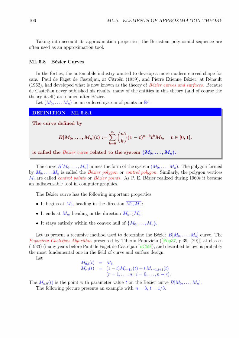
106 ML.5. ELEMENTS OF APPROXIMATION THEORY
Taking into account its approximation properties, the Bernstein polynomial sequence areoften used as an approximation tool.
ML.5.8 Bezier Curves
In the forties, the automobile industry wanted to develop a more modern curved shape forcars. Paul de Faget de Casteljau, at Citroen (1959), and Pierre Etienne Bezier, at Renault(1962), had developed what is now known as the theory of Bezier curves and surfaces. Becausede Casteljau never published his results, many of the entities in this theory (and of course thetheory itself) are named after Bezier.
Let (M0, . . . ,Mn) be an ordered system of points in Rp.
DEFINITION ML.5.8.1
The curve defined by
B[M0, . . . , Mn](t) :=n∑
k=0
(n
k
)
(1 − t)n−ktkMk, t ∈ [0, 1].
is called the Bezier curve related to the system (M0, . . . , Mn).
The curve B[M0, . . . ,Mn] mimes the form of the system (M0, . . . ,Mn). The polygon formedby M0, . . . ,Mn is called the Bezier polygon or control polygon. Similarly, the polygon verticesMi are called control points or Bezier points. As P. E. Bezier realized during 1960s it becamean indispensable tool in computer graphics.
The Bezier curve has the following important properties:
• It begins at M0, heading in the direction M0,M1 ;
• It ends at Mn, heading in the direction Mn−1Mn ;
• It stays entirely within the convex hull of {M0, . . . ,Mn}.
Let us present a recursive method used to determine the Bezier B[M0, . . . ,Mn] curve. ThePopoviciu-Casteljau Algorithm presented by Tiberiu Popoviciu ([Pop37, p.39, (29)]) at classes(1933) (many years before Paul de Faget de Casteljau [dC59]), and described below, is probablythe most fundamental one in the field of curve and surface design.
LetM0,i(t) = Mi,Mr,i(t) = (1− t)Mr−1,i(t) + tMr−1,i+1(t)
(r = 1, . . . , n; i = 0, . . . , n − r).
The Mn,0(t) is the point with parameter value t on the Bezier curve B[M0, . . . ,Mn].The following picture presents an example with n = 3, t = 1/3.
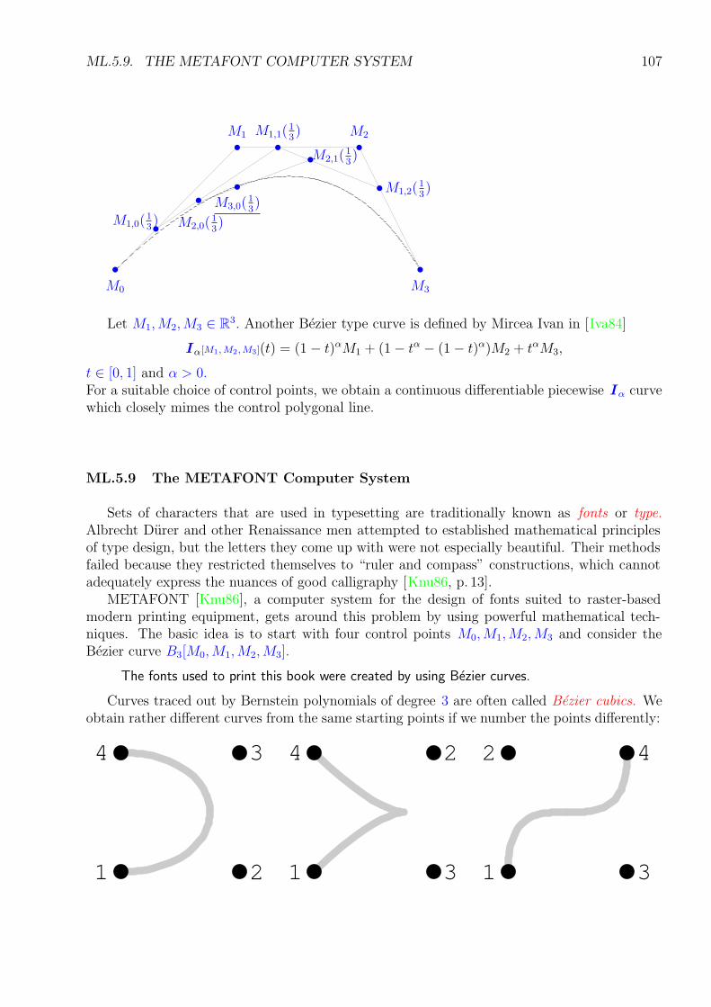
ML.5.9. THE METAFONT COMPUTER SYSTEM 107
•
•
• • •
•
•
••
M1,0(13)
M1 M1,1(13) M2
M1,2(13)
M3M0
M2,0(13)
M3,0(13)
M2,1(13)•
Let M1,M2,M3 ∈ R3. Another Bezier type curve is defined by Mircea Ivan in [Iva84]
Iα[M1, M2, M3](t) = (1− t)αM1 + (1− tα − (1− t)α)M2 + tαM3,
t ∈ [0, 1] and α > 0.For a suitable choice of control points, we obtain a continuous differentiable piecewise Iα curvewhich closely mimes the control polygonal line.
ML.5.9 The METAFONT Computer System
Sets of characters that are used in typesetting are traditionally known as fonts or type.Albrecht Durer and other Renaissance men attempted to established mathematical principlesof type design, but the letters they come up with were not especially beautiful. Their methodsfailed because they restricted themselves to “ruler and compass” constructions, which cannotadequately express the nuances of good calligraphy [Knu86, p. 13].
METAFONT [Knu86], a computer system for the design of fonts suited to raster-basedmodern printing equipment, gets around this problem by using powerful mathematical tech-niques. The basic idea is to start with four control points M0,M1,M2,M3 and consider theBezier curve B3[M0,M1,M2,M3].
The fonts used to print this book were created by using Bezier curves.
Curves traced out by Bernstein polynomials of degree 3 are often called Bezier cubics. Weobtain rather different curves from the same starting points if we number the points differently:
1 2
34
1
2
3
4
1 3
42
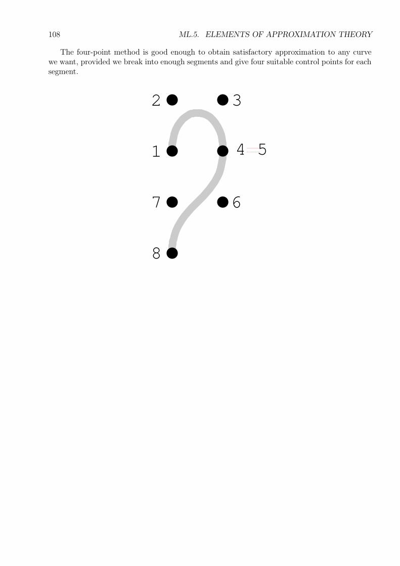
108 ML.5. ELEMENTS OF APPROXIMATION THEORY
The four-point method is good enough to obtain satisfactory approximation to any curvewe want, provided we break into enough segments and give four suitable control points for eachsegment.
1
2 3
4 5
67
8
ML.6
Integration of Ordinary DifferentialEquations
ML.6.1 Introduction
Equations involving one or several derivatives of a function are called ordinary differentialequations. A problem involving ordinary differential equations is not completely specified byits equations. Even more important in determining how to solve the problem numerically isthe nature of the problem’s boundary conditions.
Boundary conditions can be divided into two broad categories:
• Initial value problems;
• Two-point boundary value problems.
Let f : [a, b]× [c, d]→ R be a continuous function possessing continuous partial derivatives oforder two.
We will consider the following initial value problem:{
dy
dt= f(t, y)
y(a) = y0,t ∈ [a, b], (6.1.1)
which has a unique solution y ∈ C2[a, b].Define
h =b− a
n, ti = a + ih, i = 0, . . . , n,
where n is a positive integer. Some numerical methods for solving the initial value problem( 6.1.1 ) will be presented.
ML.6.2 The Euler Method
Expand the solution y of the problem ( 6.1.1 ) into a Taylor series,
y(ti+1) = y(ti) + hy′(ti) +h2
2y′′(ξi),
109
110 ML.6. INTEGRATION OF ORDINARY DIFFERENTIAL EQUATIONS
ti < ξi < ti+1, i = 0, . . . , n − 1. But y′(t) = f(t, y(t)), and hence
y(ti+1) = y(ti) + hf(ti, y(ti)) +h2
2y′′(ξi).
The Euler Method can be obtained by neglecting the remainder termh2
2y′′(ξi), in the above
expansionyi+1 = yi + hf(ti, yi), i = 0, . . . , n − 1. (6.2.1)
The Euler method is one of the oldest and best known numerical method for integratingdifferential equations. It can be improved in a number of ways.
ML.6.3 The Taylor Series Method
Suppose that equation ( 6.1.1 ) has a solution y ∈ Cp+1[a, b]. Also y(ti+1) is approximatedby a Taylor polynomial
y(ti) + hy′(ti) + ∙ ∙ ∙ +hp
p!y(p)(ti).
Use the relations:y′(t) = f(t, y(t)),
y′′(t) = f ′t(t, y(t)) + f ′
y(t, y(t)) ∙ f(t, y(t)), etc.,
and denote by Tp(t, v) the expression obtained by replacing y(t) by v in
gp(t) =
p−1∑
j=0
hj+1
(j + 1)!
d
dt
j
(f(t, y(t))).
We obtain a Taylor method of order p :
yi+1 = yi + Tp(ti, yi), i = 0, . . . , n − 1. (6.3.1)
For p = 1, we have
g1(t) = h f(t, y(t)), T1(t, v) = h f(t, v),
hence we obtain the Euler’s method:
yi+1 = yi + h f(ti, yi), i = 0, . . . , n − 1.
For p = 2, we get
g2(t) = h f(t, y(t)) +h2
2
d
dtf(t, y(t))
= h f(t, y(t)) +h2
2
(f ′
t(t, y(t)) + f ′y(t, y(t)) ∙ f(t, y(t))
),
ML.6.4. THE RUNGE-KUTTA METHOD 111
hence
T2(t, v) = h f(t, v) +h2
2
(f ′
t(t, v) + f ′y(t, v) ∙ f(t, v)
),
and we obtain the Taylor method of order two:
yi+1 = yi + h f(ti, yi) +h2
2
(f ′
t(ti, yi) + f ′y(ti, yi) ∙ f(ti, yi)
),
i = 0, . . . , n − 1.
ML.6.4 The Runge-Kutta Method
Let y be a solution of equation ( 6.1.1 ). The constants
a1, . . . , ap, b1, . . . , bp−1, c11, c21, c22 . . . , cp−1,p−1,
given in the relations:
k1 = h f(ti, y(ti)),k2 = h f(ti + b1h, y(ti) + c11k1),. . . . . .kp = h f(ti + bp−1h, y(ti) + cp−1,1k1 + ∙ ∙ ∙ + cp−1,p−1kp−1),
will be determined such that the functions:
h 7→ y(ti + h), and h 7→ y(ti) + a1k1 + ∙ ∙ ∙ + apkp,
have the same Taylor approximation of order o(hp).For example, when p = 2, we need only to find the constants
a1, a2, b1, c11,
given in the relations: {k1 = h f(ti, y(ti)),k2 = h f(ti + b1h, y(ti) + c11k1),
such that the two functions:
h 7→ y(ti + h), and h 7→ y(ti) + a1k1 + a2k2,
have the same Taylor approximation of order o(h2).The approximation of order o(h2) of the function
y(ti+1) = y(ti + h)
isy(ti) + y′(ti) h + y′′(ti)
h2
2
= y(ti) + f(ti, y(ti)) h + (f ′t(ti, y(ti)) + f ′
y(ti, y(ti)) f(ti, y(ti)))h2
2,
and the approximation of order o(h2) of the function
y(ti) + a1k1 + a2k2
= y(ti) + a1h f(ti, y(ti)) + a2h f(ti + b1h, y(ti) + c11k1),
112 ML.6. INTEGRATION OF ORDINARY DIFFERENTIAL EQUATIONS
isy(ti) + a1h f(ti, y(ti))
+a2h(f(ti, y(ti)) + b1h f ′t(ti, y(ti)) + c11k1f
′y(ti, y(ti)) f(ti, y(ti)))
= y(ti) + (a1 + a2)f(ti, y(ti))) h+(a2b1f
′t(ti, y(ti)) + a2c11f
′y(ti, y(ti)) f(ti, y(ti))) h2.
Consequently, we obtain the system
a1 + a2 = 1a2b1 = 1
2
a2c11 = 12
,
hence, by taking a1 = 12, we obtain:
a2 =1
2, b1 = 1, c11 = 1.
The Runge-Kutta algorithm of order two can be defined by the equations:
y0 = y(t0)
k1 = h f(ti, yi)k2 = h f(ti + h, yi + k1)yi+1 = yi + 1
2(k1 + k2)
i = 0, . . . , n − 1.
The classical Runge-Kutta method (that of order four), can be defined by the followingequations:
y0 = y(t0)
k1 = h f(ti, yi)k2 = h f(ti + 1
2h, yi + 1
2k1)
k3 = h f(ti + 12h, yi + 1
2k2)
k4 = h f(ti + h, yi + k3)yi+1 = yi + 1
6(k1 + 2k2 + 2k3 + k4)
i = 0, . . . , n − 1.
ML.6.5 The Runge-Kutta Method for Systems of Equations
Consider the system of differential equations
dx1
dt= f1(t, x1, . . . , xn)
......
dxn
dt= fn(t, x1, . . . , xn)
. (6.5.1)
with initial conditions: x1(t0) = x01, . . . , xn(t0) = x0
n.Using the notations
F = [f1, . . . , fn], X = [x1, . . . , xn],
system ( 6.5.1 ) can be written in the form
dX
dt= F (t,X),
ML.6.5. THE RUNGE-KUTTA METHOD FOR SYSTEMS OF EQUATIONS 113
with the initial condition X(t0) = X0 = [x01, . . . , x
0n].
The Runge-Kutta method of order four for system ( 6.5.1 ) is:
X0 = X(t0)
K1 = hF (ti, Xi)K2 = hF (ti + 1
2h,Xi + 1
2K1)
K3 = hF (ti + 12h,Xi + 1
2K2)
K4 = hF (ti + h,Xi + K3)Xi+1 = Xi + 1
6(K1 + 2K2 + 2K3 + K4)
i = 0, . . . , n − 1.

114
ML.7
Integration of Partial DifferentialEquations
ML.7.1 Introduction
Partial differential equations (PDE) are at the heart of many computer analysis and simu-lations of continuous physical systems.
The intend of this chapter is to give the briefest possible useful introduction. We limit ourtreatment to partial differential equations of order two. A linear partial differential equation oforder two has the following form
A∂2u
∂x2+ 2B
∂2u
∂x∂y+ C
∂2u
∂y2+ D
∂u
∂x+ E
∂u
∂y+ F u + G = H, (7.1.1)
where the coefficients A,B, . . . , H are functions of x and y. Equation ( 7.1.1 ) is called homo-geneous when H = 0. Otherwise it is called nonhomogeneous. For a given domain, in mostmathematical books, the partial differential equations are classified, on the basis of their dis-criminant Δ = B2 − AC, into three categories:
• elliptic, if Δ < 0;
• parabolic, if Δ = 0;
• hyperbolic, if Δ > 0.
A general method to approximate the solution is the grid method. The first step is to chooseintegers n, m, and step sizes h, k such that
h =b− a
n, k =
d− c
m.
Partitioning the interval [a, b] into n equal parts of width h and the interval [c, d] into m equalparts of width k provides a grid by drawing vertical and horizontal lines through the pointswith coordinates (xi, yj), where
xi = a + ih, yj = c + jk,
115
116 ML.7. INTEGRATION OF PARTIAL DIFFERENTIAL EQUATIONS
i = 0, . . . , n; j = 0, . . . ,m. The lines x = xi, y = yj , are called grid lines, and their intersectionsare the mesh points of the grid.
ML.7.2 Parabolic Partial-Differential Equations
Consider a particular case of the heat or diffusion parabolic partial differential equation
∂u
∂t(x, t) =
∂2u
∂x2(x, t), 0 < x < l, 0 < t < T
subject to conditionsu(0, t) = u(l, t) = 0, 0 < t < Tu(x, 0) = f(x), 0 ≤ x ≤ l,
One of the algorithms used to approximate the solution of this equation is the Crank-Nicolson algorithm.
It is an implicit algorithm defined by the relations:
∂u
∂t(ih, jk) ≈
ui,j+1 − uij
k,
∂2u
∂x2(ih, jk) ≈
ui+1,j+1 − 2ui,j+1 + ui−1,j+1 + ui+1,j − 2uij + ui−1,j
2h2.
By letting r = kh2 , we obtain the system:
2(1 + r)ui,j+1 − rui−1,j+1 − rui+1,j+1 = rui−1,j + 2(1− r)uij + rui+1,j .
The values in the nodes of the line “j + 1” are calculated using the already computed values inthe line “j”.
ML.7.3 Hyperbolic Partial Differential Equations
For this type of PDE, we consider the numerical solution of particular case of the waveequation:
∂2u
∂t2(x, t) =
∂2u
∂x2(x, t), 0 < x < l, 0 < t < T,
subject to conditionsu(0, t) = u(l, t) = 0, 0 < t < T,u(x, 0) = f(x), 0 ≤ x ≤ l,∂u
∂t(x, 0) = g(x), 0 ≤ x ≤ l
Using the finite difference method consider
∂2u
∂x2(ih, jk) =
ui+1,j − 2uij + ui−1,j
h2,
∂2u
∂y2(ih, jk) =
ui,j+1 − 2uij + ui,j−1
k2,
hence, letting r =k2
h2, we obtain an explicit algorithm
ui,j+1 = −ui,j−1 + 2(1− r)uij + r(ui+1,j + ui−1,j).
ML.7.4. ELLIPTIC PARTIAL DIFFERENTIAL EQUATIONS 117
ML.7.4 Elliptic Partial Differential Equations
The approximate solution of the Poisson elliptic partial differential equation
∂2u
∂x2(x, y) +
∂2u
∂y2(x, y) = f(x, y), x ∈ [a, b], y ∈ [c, d]
subject to boundary conditionsu(x, c) = f(x), u(x, d) = g(x), x ∈ [a, b],u(a, y) = f(y), u(b, y) = g(y), y ∈ [c, d].
can be found by taking h = k,
∂2u
∂x2(ih, jh) =
ui+1,j − 2uij + ui−1,j
h2,
∂2u
∂y2(ih, jh) =
ui,j+1 − 2uij + ui,j−1
h2,
Denoting r =k2
h2, we obtain an implicit algorithm
ui−1,j + ui+1,j + ui,j−1 + ui,j+1 − 4uij = fij .

118
ML.7
Self Evaluation Tests
ML.7.1 Tests
Let x0, . . . , xn be distinct points on the real axis, f be a function defined on these pointsand `(x) = (x− x0) . . . (x− xn).
TEST ML.7.1.1
Let P be a polynomial. The remainder obtained by dividing the polynomial Pby the polynomial (X − x0) . . . (X − xn) is:
(A) The Lagrange Polynomial L(x0, . . . , xn; P );
(B) The Lagrange Polynomial L(x0, . . . , xn; (X − x0) . . . (X − xn));
(C) The Lagrange Polynomial L(x0, . . . , xn; Xn);
(D) The Lagrange Polynomial L(x0, . . . , xn; Xn P )
TEST ML.7.1.2
The polynomial L(x0, . . . , xn; Xn+1) is:
(A) Xn+1;
(B) Xn+1 − (X − x0)(X − x1) . . . (X − xn);
(C) Xn;
(D) 0;
119
120 ML.7. SELF EVALUATION TESTS
TEST ML.7.1.3
Let Pn : R → R be a polynomial of degree at most n, n ∈ N. Prove thedecomposition in partial fractions
Pn(x)
(x − x0) . . . (x − xn)=
n∑
k=0
1
x − xi∙
P (xi)
`′(xi).
TEST ML.7.1.4
Calculate the sum
n∑
i=0
xki(xi − x0) . . . (xi − xi−1)(xi − xi+1) . . . (xi − xn)
,
k = 0, . . . , n.
TEST ML.7.1.5
Calculate [x0, . . . , xn; xn+1].
TEST ML.7.1.6
Calculate[x0, . . . , xn; (X − x0) . . . (X − xk)],
k ∈ N.
TEST ML.7.1.7
Prove that
L(x0, . . . , xn; L(x1, . . . , xn; f)) = L(x1, . . . , xn; L(x0, . . . , xn; f)).
TEST ML.7.1.8
Prove that, for x /∈ {x0, . . . , xn},
[
x0, . . . , xn;f(t)
x − t
]
t
=L(x0, . . . , xn; f)(x)
(x − x0) . . . (x − xn).
ML.7.1. TESTS 121
TEST ML.7.1.9
If f(x) = 1x
and 0 < x0 < x1 < ∙ ∙ ∙ < xn, then
[x0, . . . , xn; f ] =(−1)n
x0 . . . xn.
TEST ML.7.1.10
For x > 0, we define the function
H(x) = 1 +∞∑
k=1
1
(x + 2) . . . (x + k + 1).
Show that
a) H(x) = e(x + 1)J(x), where
J(x) =
∫ 1
0
e−ttxdt.
b) e1x+2 ≤ H(x) ≤ e+x+1
x+2.
TEST ML.7.1.11
a) Show that the following quadrature formula
∫ 1
0
f(x)dx =1
4f(0) +
3
4f
(2
3
)
+ R(f)
has the degree of exactness 2.
b) Let f be a function from C1[0, 1]. Show that there exists a point θ = θ(f)such that
R(f) =1
36
[
θ, θ, 0,2
3; f
]
.
122 ML.7. SELF EVALUATION TESTS
TEST ML.7.1.12
Show that the following quadrature formula
∫ b
a
f(x)dx =b − a
4
[
f(a) + 3f
(a + 2b
3
)]
+ R(f)
has the degree of exactness 2 and for f ∈ C3[a, b], there exists c = c(f) ∈ [a, b]such that
R(f) =(b − a)4
216f ′′′(c).
TEST ML.7.1.13
Let f ∈ C3[a, b] and let us consider the following quadrature formula
∫ b
a
f(x)dx =b − a
4n
n−1∑
k=0
[
f
(
a +k(b − a)
n
)
+ 3f
(
a +(3k + 2)(b − a)
3n
)]
.
Show that
limn→∞
n3Rn(f) =(b − a)3
216[f ′′(b) − f ′′(a)] .
TEST ML.7.1.14
Let Π+2n be the set of all polynomials of degree 2n which are positive on the set
{
cos(2k + 1)π
2n
∣∣∣ k = 0, 1, ..., n − 1
}
and having the leading coefficient 1. Using the gaussian quadrature formula:
∫ 1
−1
f(x)√
1 − x2dx =
n−1∑
k=0
Akf
(
cos(2k + 1)π
2n
)
+ Rn(f),
show that
infP∈Π
+2n
∫ 1
−1
P (x)√
1 − x2dx =
π
22n−1.
ML.7.1. TESTS 123
TEST ML.7.1.15
Find a quadrature formula of the following form
∫ 1
0
f(x)dx = Af(0) + Bf(x1) + Cf(x2) + R(f), x1 6= x2, x1, x2 ∈ (0, 1),
with maximum degree of exactness.
TEST ML.7.1.16
Find a quadrature formula of the form
∫ 1
0
f(x)dx
= c1
(
f
(1
2− x1
)
+ f
(1
2+ x1
))
+ c2
(
f ′(
1
2− x1
)
− f ′(
1
2+ x1
))
+R(f),
f ∈ C1[0, 1] with maximum degree of exactness.
TEST ML.7.1.17
Let Pn(x) = xn + a1xn−1 + ∙ ∙ ∙ + an a polynomial with real coefficients. Show
that ∫ 1
0
P 2n(x)dx ≥
(n!)5
[(2n)!]2(2n + 1).
For what polynomial does the inequality above become equality?
124 ML.7. SELF EVALUATION TESTS
ML.7.2 Answers to Tests
TEST ANSWER ML.7.1.1
Answer (A). Indeed, let P (x) = Q(x) (x − x0) . . . (x − xn) + R(x). We have
R(xi) = P (xi), i = 0, . . . , n.
Since the degree of the polynomial R is at most n, we get R = L(x0, . . . , xn; P ).
TEST ANSWER ML.7.1.2
Answer (B). Indeed, we have
Xn+1 = 1 ∙ (X − x0)(X − x1) . . . (X − xn)
+Xn+1 − (X − x0)(X − x1) . . . (X − xn).
By Test (ML.7.1.1 ), we obtain
L(x0, . . . , xn; Xn+1) = Xn+1 − (X − x0)(X − x1) . . . (X − xn).
TEST ANSWER ML.7.1.3
Since the Lagrange operator L(x0, . . . , xn; ∙) preserves polynomials with degreeat most n, with `(x) = (x − x0) . . . (x − xn), we have
Pn(x)
`(x)=
L(x0, . . . , xn; Pn)(x)
`(x)=
n∑
k=0
1
x − xi∙
P (xi)
`′(xi).
TEST ANSWER ML.7.1.4
n∑
i=0
xki(xi − x0) . . . (xi − xi−1)(xi − xi+1) . . . (xi − xn)
= [x0, . . . , xn; Xk]
=
{0, if 0 ≤ k ≤ n − 1;1, if k = n.
See( 3.3.2 ).
ML.7.2. ANSWERS TO TESTS 125
TEST ANSWER ML.7.1.5
We have:
0 = [x0, . . . , xn; (X − x0) . . . (X − xn)]
= [x0, . . . , xn; Xn+1 − (x0 + ∙ ∙ ∙ + xn)X
n + ∙ ∙ ∙]
= [x0, . . . , xn; Xn+1] − (x0 + ∙ ∙ ∙ + xn)[x0, . . . , xn; X
n] + 0
= [x0, . . . , xn; Xn+1] − (x0 + ∙ ∙ ∙ + xn) ∙ 1
Consequently
[x0, . . . , xn; Xn+1] = x0 + ∙ ∙ ∙ + xn.
TEST ANSWER ML.7.1.6
For k < n, the degree of the polynomial (X − x0) . . . (X − xk−1) is at mostn − 1, hence
[x0, . . . , xn; (X − x0) . . . (X − xk−1)] = 0.
For k = n,
[x0, . . . , xn; (X − x0) . . . (X − xn−1)]
= [x0, . . . , xn; Xn − ∙ ∙ ∙]
= [x0, . . . , xn; Xn]−0
= 1.
For k > n, the polynomial (X − x0) . . . (X − xk−1) takes zero value for X =x0, . . . xn, hence
[x0, . . . , xn; (X − x0) . . . (X − xk−1)] = 0.
126 ML.7. SELF EVALUATION TESTS
TEST ANSWER ML.7.1.7
Since the degree of the polynomial L(x1, . . . , xn; f) is at most n − 1, we have
L(x0, . . . , xn; L(x1, . . . , xn; f)) = L(x1, . . . , xn; f).
Consider the polynomial
P = L(x1, . . . , xn; L[x0, . . . , xn; f ]).
We have:
P (xi) = L(x1, . . . , xn; L[x0, . . . , xn; f ])(xi)
= L[x0, . . . , xn; f ](xi), i = 1, . . . , n
= f(xi), i = 1, . . . , n,
henceP = L(x1, . . . , xn; f).
TEST ANSWER ML.7.1.8
With `(x) = (x − x0) . . . (x − xn), we have
L(x0, . . . , xn; f)(x) =n∑
k=0
`(x)
x − xi∙
f(xi)
`′(xi),
henceL(x0, . . . , xn; f)(x)
`(x)=
n∑
k=0
f(xi)
x−xi
`′(xi)=
[
x0, . . . , xn;f(t)
x − t
]
t
.
ML.7.2. ANSWERS TO TESTS 127
TEST ANSWER ML.7.1.9
By using problem ( ML.3.12.8 ), we have
[
x0, . . . , xn;1
t
]
t
= −L(x0, . . . , xn; 1)(0)
(0 − x0) . . . (0 − xn)=
(−1)n
x0 . . . xn.
Solution 2. We write the obvious equality
[
x0, . . . , xn;(t − t0) . . . (t − xn)
t
]
= 0
in the form[
x0, . . . , xn; tn − (t0 + ∙ ∙ ∙ + tn)t
n−1 + ∙ ∙ ∙ + (−1)n+1t0 . . . xn
t
]
= 0,
i.e.,
1 − (t0 + ∙ ∙ ∙ + tn)0 + ∙ ∙ ∙ + 0 + (−1)n+1t0 . . . xn
[
x0, . . . , xn;1
t
]
= 0.
128 ML.7. SELF EVALUATION TESTS
TEST ANSWER ML.7.1.10
a) We have,
1
(x + 2)...(x + k + 1)=
Γ(x + 2)Γ(k)
Γ(x + k + 2)
1
(k − 1)!. (7.2.1)
From (7.2.1), we get
H(x) = 1 +∞∑
k=1
β(x + 2, k)1
(k − 1)!
= 1 +∞∑
k=1
1
(k − 1)!
∫ 1
0
tk−1(1 − t)x+1dt = 1 +
∫ 1
0
∞∑
k=0
1
k!tk(1 − t)x+1dt
= 1 +
∫ 1
0
et(1 − t)x+1dt = 1 + e
∫ 1
0
e−ttx+1.
Integrating by parts, we obtain
H(x) = 1 + e
[
−e−ttx+1∣∣∣10
+ (x + 1)
∫ 1
0
e−ttxdt
]
or,
H(x) = e(x + 1)
∫ 1
0
e−ttxdt.
b) The function e−t is a convex function. We consider the weight functionw(t) = (x + 1)tx, t ∈ [0, 1] and the quadrature formula
∫ 1
0
w(t)f(t)dt = f
(x + 1
x + 2
)
+ R(f),
with x ≥ 0 fixed. The above quadrature formula is a Gauss-type quadratureformula. Let f be a convex function. Then, R(f) ≥ 0. For f(t) = e−t, weobtain
H(x) ≥ e ∙ e−x+1x+2 or H(x) ≥ e
1x+2 .
For the second inequality we use the trapezoidal rule with the weight functiongiven by w. We obtain
H(x) ≤ e
[
1 −∫ 1
0
(x + 1)tx+1dt + e−1
∫ 1
0
(x + 1)tx+1dt
]
=e + x + 1
x + 2.
ML.7.2. ANSWERS TO TESTS 129
TEST ANSWER ML.7.1.11
a) We have
R(e0) =
∫ 1
0
dx −1
4−
3
4= 0, R(e1) =
∫ 1
0
xdx −3
4
2
3= 0
R(e2) =
∫ 1
0
x2dx −3
4
4
9= 0, R(e3) =
∫ 1
0
x3dx −8
27
3
4=
1
36.
b) For the beginning, we remark that
f(x) − f
(2
3
)
=
(
x −2
3
) [
x,2
3; f
]
,
∫ 1
0
x
(
x −2
3
)
dx = 0 (7.2.2)
From (7.2.2), we obtain
∫ 1
0
x
(
x −2
3
)
f(x)dx =
∫ 1
0
x
(
x −2
3
)2 [
x,2
3; f
]
dx. (7.2.3)
Using the mean value theorem for integrals in (7.2.3), implies that there existsa point c = c(f) ∈ [0, 1] such that
∫ 1
0
x
(
x −2
3
)
f(x)dx =
[
c,2
3; f
] ∫ 1
0
x
(
x −2
3
)2
dx =1
36
[
c,2
3; f
]
Applying the mean value theorem for divided differences in (7.2.4), it followsthat there exists a point θ = θ(f) ∈ [0, 1] such that
∫ 1
0
x
(
x −2
3
)
f(x)dx =1
36f ′(θ). (7.2.4)
The quadrature formula is an interpolation type formula and therefore R(f) =∫ 1
0
x
(
x −2
3
) [
x, 0,2
3; f
]
dx. From (7.2.4), we get
∫ 1
0
x
(
x −2
3
) [
x, 0,2
3; f
]
dx =1
36
[
x, 0,2
3; f
]′
x=θ
. (7.2.5)
On the other hand, we have
[
x, 0,2
3; f
]′=
[
x, x, 02
3; f
]
.From here, by using
(7.2.5), we obtain R(f) =1
36
[
θ, θ, 0,2
3; f
]
.
130 ML.7. SELF EVALUATION TESTS
TEST ANSWER ML.7.1.12
A simple computation shows that
R(ei) =
∫ b
a
xidx −b − a
4
[
ai + 3
(a + 2b
3
)i]
= 0,
for i = 0, 1, 2 and
R(e3) =(b − a)4
36.
Let us consider the function g : [0, 1] → R defined by g(t) = f((1 − t)a + bt).Using previous results (Test ML.7.1.11), we have
R(g) =1
36
[
θ, θ, 0,2
3; g
]
.
Using the mean value theorem for divided differences, it follows that there existsa point c = c(f) ∈ [0, 1] such that
[
θ, θ, 0,2
3; g
]
=g′′(c)
6.
We haveg′′′(t) = (b − a)3f ′′′((1 − t)a + tb)
and ∫ 1
0
g(t)dt =1
4
[
g(0) + 3g
(2
3
)]
+g′′′(c)
216
or
∫ 1
0
f((1 − t)a + tb)dt =1
4
[
f(a) + 3f
(a + 2b
3
)]
+(b − a)3f ′′′(c)
216.
If we make the change of variable x = (1 − t)a + tb, we get
∫ b
a
f(x)dx =b − a
4
[
f(a) + 3f
(a + 2b
3
)]
+(b − a)4f ′′′(c)
216.
ML.7.2. ANSWERS TO TESTS 131
TEST ANSWER ML.7.1.13
Let xk be the points given by
xk = a + kb − a
n, k = 0, n.
Then ∫ b
a
f(x)dx =n∑
k=1
∫ xk
xk−1
f(x)dx.
But,
∫ xk
xk−1
f(x)dx =b − a
4n
[
f(xk−1) + 3f
(xk−1 + 2xk
3
)]
+(b − a)4
216n4f ′′′ (ck,n) .
(7.2.6)Since ck,n ∈ [xk−1, xk], k = 1, n,
b − a
n
n∑
k=1
f ′′′ (ck,n)
is a Riemann sum for the function f ′′′(∙), relative to the division
Δn : a = x0 < x1 < ... < xn = b.
From (7.2.6), we get
limn→∞
n3Rn(f) =(b − a)3
216limn→∞
b − a
n
n∑
k=1
f ′′′ (ck,n)
=(b − a)3
216
∫ b
a
f ′′′(x)dx
=(b − a)3
216[f ′′(b) − f ′′(a)] .
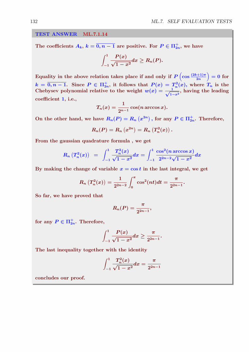
132 ML.7. SELF EVALUATION TESTS
TEST ANSWER ML.7.1.14
The coefficients Ak, k = 0, n − 1 are positive. For P ∈ Π+2n, we have
∫ 1
−1
P (x)√
1 − x2dx ≥ Rn(P ).
Equality in the above relation takes place if and only if P(cos (2k+1)π
2n
)= 0 for
k = 0, n − 1. Since P ∈ Π+2n, it follows that P (x) = T 2
n(x), where Tn is theChebysev polynomial relative to the weight w(x) = 1√
1−x2, having the leading
coefficient 1, i.e.,
Tn(x) =1
2n−1cos(n arccos x).
On the other hand, we have Rn(P ) = Rn(x2n
), for any P ∈ Π+
2n. Therefore,
Rn(P ) = Rn(x2n
)= Rn
(T 2n(x)
).
From the gaussian quadrature formula , we get
Rn(T 2n(x)
)=
∫ 1
−1
T 2n(x)
√1 − x2
dx =
∫ 1
−1
cos2(n arccos x)
22n−2√
1 − x2dx
By making the change of variable x = cos t in the last integral, we get
Rn(T 2n(x)
)=
1
22n−2
∫ π
0
cos2(nt)dt =π
22n−1.
So far, we have proved that
Rn(P ) =π
22n−1,
for any P ∈ Π+2n. Therefore,
∫ 1
−1
P (x)√
1 − x2dx ≥
π
22n−1.
The last inequality together with the identity
∫ 1
−1
T 2n(x)
√1 − x2
dx =π
22n−1
concludes our proof.
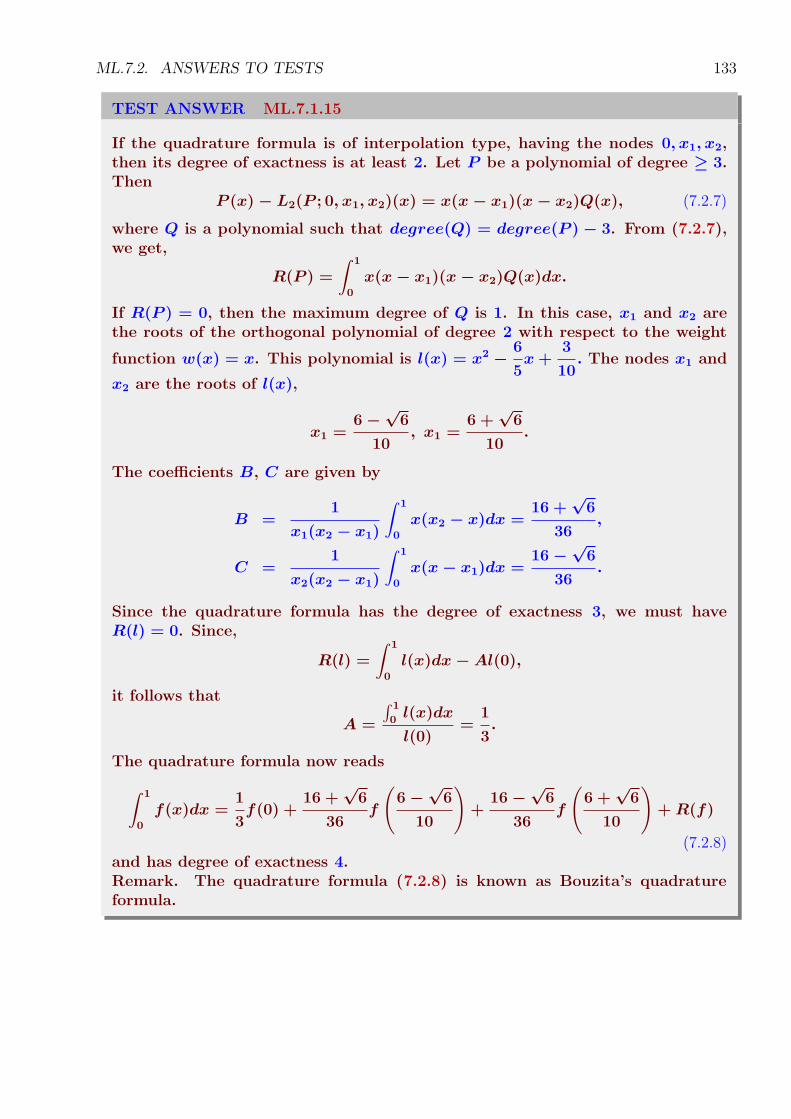
ML.7.2. ANSWERS TO TESTS 133
TEST ANSWER ML.7.1.15
If the quadrature formula is of interpolation type, having the nodes 0, x1, x2,then its degree of exactness is at least 2. Let P be a polynomial of degree ≥ 3.Then
P (x) − L2(P ; 0, x1, x2)(x) = x(x − x1)(x − x2)Q(x), (7.2.7)
where Q is a polynomial such that degree(Q) = degree(P ) − 3. From (7.2.7),we get,
R(P ) =
∫ 1
0
x(x − x1)(x − x2)Q(x)dx.
If R(P ) = 0, then the maximum degree of Q is 1. In this case, x1 and x2 arethe roots of the orthogonal polynomial of degree 2 with respect to the weight
function w(x) = x. This polynomial is l(x) = x2 −6
5x +
3
10. The nodes x1 and
x2 are the roots of l(x),
x1 =6 −
√6
10, x1 =
6 +√
6
10.
The coefficients B, C are given by
B =1
x1(x2 − x1)
∫ 1
0
x(x2 − x)dx =16 +
√6
36,
C =1
x2(x2 − x1)
∫ 1
0
x(x − x1)dx =16 −
√6
36.
Since the quadrature formula has the degree of exactness 3, we must haveR(l) = 0. Since,
R(l) =
∫ 1
0
l(x)dx − Al(0),
it follows that
A =
∫ 1
0l(x)dx
l(0)=
1
3.
The quadrature formula now reads
∫ 1
0
f(x)dx =1
3f(0) +
16 +√
6
36f
(6 −
√6
10
)
+16 −
√6
36f
(6 +
√6
10
)
+ R(f)
(7.2.8)and has degree of exactness 4.Remark. The quadrature formula (7.2.8) is known as Bouzita’s quadratureformula.
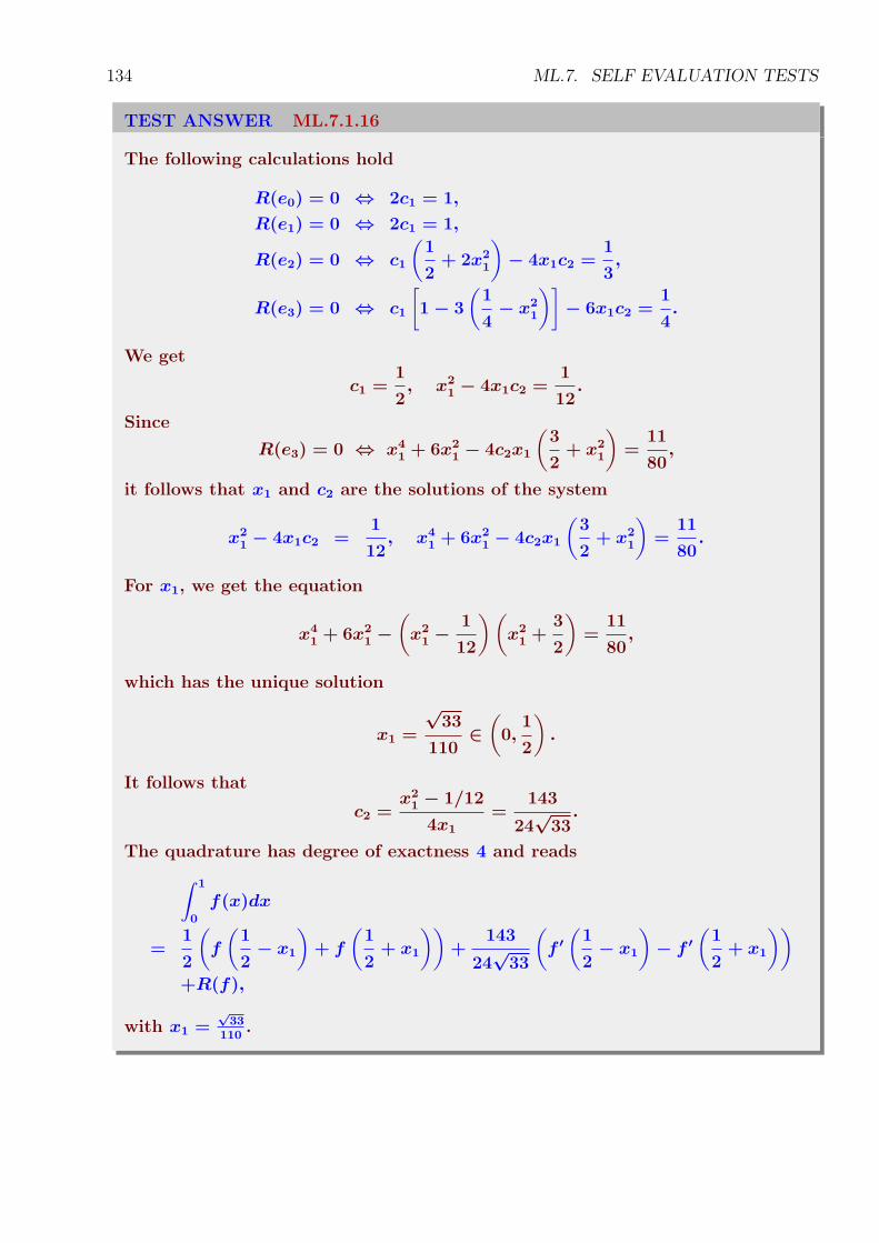
134 ML.7. SELF EVALUATION TESTS
TEST ANSWER ML.7.1.16
The following calculations hold
R(e0) = 0 ⇔ 2c1 = 1,
R(e1) = 0 ⇔ 2c1 = 1,
R(e2) = 0 ⇔ c1
(1
2+ 2x2
1
)
− 4x1c2 =1
3,
R(e3) = 0 ⇔ c1
[
1 − 3
(1
4− x2
1
)]
− 6x1c2 =1
4.
We get
c1 =1
2, x2
1 − 4x1c2 =1
12.
Since
R(e3) = 0 ⇔ x41 + 6x2
1 − 4c2x1
(3
2+ x2
1
)
=11
80,
it follows that x1 and c2 are the solutions of the system
x21 − 4x1c2 =
1
12, x4
1 + 6x21 − 4c2x1
(3
2+ x2
1
)
=11
80.
For x1, we get the equation
x41 + 6x2
1 −
(
x21 −
1
12
)(
x21 +
3
2
)
=11
80,
which has the unique solution
x1 =
√33
110∈
(
0,1
2
)
.
It follows that
c2 =x2
1 − 1/12
4x1
=143
24√
33.
The quadrature has degree of exactness 4 and reads
∫ 1
0
f(x)dx
=1
2
(
f
(1
2− x1
)
+ f
(1
2+ x1
))
+143
24√
33
(
f ′(
1
2− x1
)
− f ′(
1
2+ x1
))
+R(f),
with x1 =√
33110
.
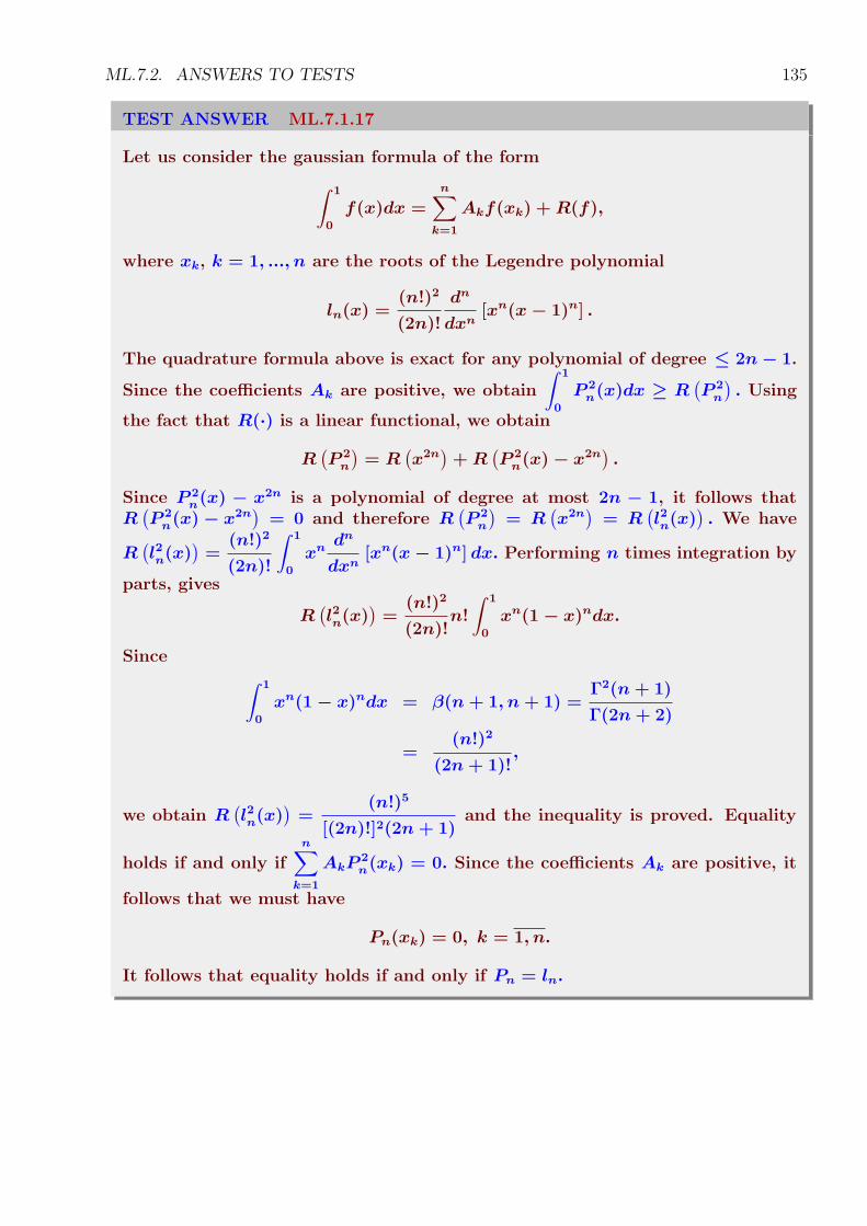
ML.7.2. ANSWERS TO TESTS 135
TEST ANSWER ML.7.1.17
Let us consider the gaussian formula of the form
∫ 1
0
f(x)dx =n∑
k=1
Akf(xk) + R(f),
where xk, k = 1, ..., n are the roots of the Legendre polynomial
ln(x) =(n!)2
(2n)!
dn
dxn[xn(x − 1)n] .
The quadrature formula above is exact for any polynomial of degree ≤ 2n − 1.
Since the coefficients Ak are positive, we obtain
∫ 1
0
P 2n(x)dx ≥ R
(P 2n
). Using
the fact that R(∙) is a linear functional, we obtain
R(P 2n
)= R
(x2n
)+ R
(P 2n(x) − x2n
).
Since P 2n(x) − x2n is a polynomial of degree at most 2n − 1, it follows that
R(P 2n(x) − x2n
)= 0 and therefore R
(P 2n
)= R
(x2n
)= R
(l2n(x)
). We have
R(l2n(x)
)=
(n!)2
(2n)!
∫ 1
0
xndn
dxn[xn(x − 1)n] dx. Performing n times integration by
parts, gives
R(l2n(x)
)=
(n!)2
(2n)!n!
∫ 1
0
xn(1 − x)ndx.
Since
∫ 1
0
xn(1 − x)ndx = β(n + 1, n + 1) =Γ2(n + 1)
Γ(2n + 2)
=(n!)2
(2n + 1)!,
we obtain R(l2n(x)
)=
(n!)5
[(2n)!]2(2n + 1)and the inequality is proved. Equality
holds if and only ifn∑
k=1
AkP2n(xk) = 0. Since the coefficients Ak are positive, it
follows that we must have
Pn(xk) = 0, k = 1, n.
It follows that equality holds if and only if Pn = ln.
Index
nk = n . . . (n + k − 1), n0 = 1,(rising factorial), 69
nk = n . . . (n− k + 1), n0 = 1,(falling factorial), 69
algorithmCooley-Tukey, 99Crank-Nicolson, 116FFT, 99Neville, 58Popoviciu-Casteljau, 106
asymptotic constant, 41
Bezier cubics, 107Bezier curves, 106BEZIER, Etienne Pierre (1910-1999), 106Bernstein polynomial, 101BERNSTEIN, Sergi Natanovich (1880–1968),
101BOOLE, George (1815–1864), 68Boolean sum, 72
CAYLEY, Arthur (1821–1895), 39CHEBYSHEV, Pafnuty Lvovich (1821–1894),
46condition number, 15correction, 20COTES, Roger(1682–1716), 83CRANK, John (born 1916) , 116
DURER, Albrecht (1471–1528), 107de CASTELJAU, Paul de Faget, 106degree of accuracy, 83divided difference, 54
eigenvalues, 37eigenvector, 37elementary functions of order n, 74equations
nonlinear, 41
nonlinear systems of, 41ordinary differential, 109
EULER, Leonhard (1707–1783), 109extrapolation, 53
Richardson, 81, 86
FADDEEV, Dmitrii Konstantinovich (1907-1989),39
Fadeev-Frame method, 39finite differences, 68fixed point, 42fonts, 107formula
Aitken-Neville, 57Gregory-Newton, 71Newton, 39Newton’s polynomial, 56simplified Newton’s, 45
GAUSS, Johann Carl Friedrich (1777–1855),20
Gauss-Seidel iterative method, 34GREGORY, James (1638–1675), 71grid, 115grid line, 116
HAMILTON, Sir William Rowan (1805–1865),39
HERMITE, Charles (1822–1901), 65HILBERT, David (1862–1943), 94
integrationRomberg, 86
interpolation, 53fundamental polynomials, 55Hermite-Lagrange polynomial, 66interpolator, 53Lagrange polynomial, 53mesh points, 53points, 53
136
INDEX 137
several variables, 71Shepard interpolant, 73
iterative techniques, 33
Jacobi’s iterative method, 34JACOBI, Carl Gustav Jacob (1804-1851), 34JORDAN, Wilhelm (1842–1899), 20
KUTTA, Martin Wilhelm (1867–1944), 111
LAGRANGE, Joseph-Louis (1736–1813), 53Le VERRIER, Urbain Jean Joseph (1811–1877),
38LEGENDRE, Adrien-Marie (1752–1833), 95LU factorization, 23
MathematicaCholeski, 32Doolittle factorization, 30Doolittle factorization “in place”, 31Eigensystem, 38Eigenvalues, 38Eigenvalues, Eigenvectors, Eigensystem, 38Eigenvectors, 38Hermite-Lagrange polynomial, 67LU factorization, 27norms, 13partitioning methods, 23pivot elimination, 19Successive Over-Relaxation, 36
matrixaugmented, 16Hilbert, 94ill-conditioned, 15lower triangular, 23norm, 10positive definite, 8strictly diagonally dominant, 7trace, 38upper triangular, 23well-conditioned, 15
mesh point, 116method
least squares, 91pivoting elimination, 17binary-search, 44bisection, 43
Chebyshev, 46Euler, 109, 110false position, 45Gauss-Jordan, 20Gauss-Seidel, 34global, 72gradient, 51grid, 115Jacobi, 34Le Verrier, 38local, 72Newton-Raphson, 44Pade, 95pivoting elimination, 16regula falsi, 45relaxation, 35Runge-Kutta, 111secant, 45Simpson, 88SOR, 35steepest descent, 51successive approximation, 42Taylor, 110Taylor series, 110
minimax problem, 91modulus of continuity, 103
NEWTON, Sir Isaac (1643–1727), 39NICOLSON, Phyllis (1917–1968), 116norm
Frobenius, 12induced, 10matrix, 10natural, 10vector, 9
operatorbackward difference, 68centered difference, 68displacement, 68forward difference, 68identity, 68shift, 68translation, 68
order of convergence, 41orthogonal set, 94orthonormal, 94
138 INDEX
PADE, Henri Eugene (1863–1953), 95partitioning methods, 20PDE, 115
elliptic, 117hyperbolic, 116parabolic, 116
pivot element, 18polynomial
characteristic, 37Chebyshev, 95Legendre, 95
quadratureGaussian, 88
quadrature formulaChebyshev’s, 83Gauss’s, 83Newton-Cotes, 87Newton-Cotes’s, 83quadrature, 83
RAPHSON, Joseph (1648–1715), 44remainder, 83RICHARDSON, Lewis Fry (1881–1953), 81rule
composite trapezoidal, 85trapezoidal, 84
RUNGE, Carle David Tolme (1856–1927), 111
scattered data, 72SCHOENBERG, Isaac Jacob (1903–1990), 74von SEIDEL, Philipp Ludwig (1821–1896), 34Shepard, Donald S.(1903–1990), 73SIMPSON, Thomas (1710–1761), 88splines, 74
B-splines, 75step size, 115stopping criterion, 42systems
nonlinear, 48, 49
TAYLOR, Brook (1685–1731), 110tensor product, 72TUKEY, John Wilder (1915–2000), 99
Vandermonde determinant, 54VANDERMONDE, Alexandre-Theophile (1735–
1796), 54
vectorresidual, 14
wave equation, 116weight function, 94
Bibliography
[Ara57] Oleg Arama. Some properties concerning the sequence of polynomials of S. N. Bernstein(in Romanian). Studii si Cerc. (Cluj), 8(3–4): 195–210, 1957.
[Bak76] N. Bakhvalov. Methodes Numeriques. Edition Mir, Moscou, 1976.
[BDL83] R. E. Barnhill, R. P. Dube, and F. F. Little. Properties of Shepard’s surfaces. RockyMountain Journal of Mathematics, 13(2): 365–382, 1983.
[BF93] Richard L. Burden and J. Douglas Faires. Numerical Analysis. PWS-KENT PublishingCompany, 1993.
[Blu72] E. K. Blum. Numerical analysis and computation theory and practice. Addison-WesleyPublishing Co., Reading, Mass.-London-Don Mills, Ont., 1972. Addison-Wesley Series inMathematics.
[Boo60] G. Boole. A treatise of the calculus of finite differences. Macmillan, Cambridge, London,1860.
[Bre83] Claude Brezinski. Outlines of Pade approximation. In H. Werner et al. eds., editor,Computational Aspects of Complex Analysis, pages 1–50. Reidel, Dordrecht, 1983.
[But87] J. C. Butcher. The numerical analysis of ordinary differential equations. A Wiley-Interscience Publication. John Wiley & Sons Ltd., Chichester, 1987. Runge-Kutta andgeneral linear methods.
[BVI95] C. Brezinski and J. Van Iseghem. A taste of Pade approximation. In Acta numerica, 1995,Acta Numer., pages 53–103. Cambridge Univ. Press, Cambridge, 1995.
[dB78] Carl de Boor. A practical guide to splines. Springer-Verlag, New York Heidelberg Berlin,1978.
[DB03a] Germund Dahlquist and Ake Bjorck. Numerical methods. Dover Publications Inc., Mineola,NY, 2003. Translated from the Swedish by Ned Anderson, Reprint of the 1974 Englishtranslation.
[dB03b] Carl de Boor. A divided difference expansion of a divided difference. J. Approx. Theory,122(1):10–12, 2003.
[dB05] Carl de Boor. Divided differences. Surveys in Approximation Theory, 1:46–69, 2005.
[dC59] Paul de Faget de Casteljau. Outilages methodes calcul. Technical report, A. Citroen, Paris,1959.
[DL93] Ronald A. DeVore and George G. Lorentz. Constructive approximation. Springer Verlag,Berlin Heidelberg New York, 1993.
139
140 BIBLIOGRAPHY
[DM72] W. S. Dorn and D. D. McCracken. Numerical Methods with FORTRAN IV Case Studies.John Wiley & Sons, Inc., New York - London - Sydney - Toronto, 1972.
[Far90] G. Farin. Curves and Surfaces for Computer Aided Geometric Design – A Practical Guide .Academic Press, Inc., Boston - San Diego - New York - London, 1990.
[Gav01] Ioan Gavrea. Aproximarea functiilor prin operatori liniari. Mediamira, Cluj-Napoca, 2001.
[Gon95] H. H. Gonska. Shepard Methoden. In Hauptseminar CAGD 1995, pages 1–34, Duisburg,1995. Gerhard Mercator Universitat.
[GZ93] H. H. Gonska and X. Zhou. Polynomial approximation with side conditions: Recent resultsand open problems. In Proc. of the First International Colloquium on Numerical Analysis,Plovdiv 1992, pages 61–71. Zeist/The Netherlands: VSP International Science Publishers,1993.
[Her78] Charles Hermite. Sur la formule d’interpolation de Lagrange. J. Reine Angew. Math.,84:70–79, 1878.
[HL89] J. Hoschek and D. Lasser. Fundamentals of Computer Aided Geometric Design. A KPeters, Ltd, 1989.
[IP92] Mircea Ivan and Kalman Pusztai. Mathematics by Computer. Comprex Publishing House,Cluj-Napoca, 1992.
[IP03] Mircea Ivan and Kalman Pusztai. Numerical Methods with Mathematica. Mediamira,Cluj-Napoca, 2003.
[Iva73] Mircea Ivan. Mean value theorems in mathematical analysis (Romanian). Master’s thesis,Babes-Bolyai University, Cluj, 1973.
[Iva82] Mircea Ivan. Interpolation Methods and Applications. PhD thesis, Babes-Bolyai University,Cluj-Napoca, 1982.
[Iva84] Mircea Ivan. On some Bernstein-Bezier type functions. In Itinerant Seminar on FunctionalEquations, Approximation and Convexity, pages 81–84, Cluj-Napoca, 1984. Babes-BolyaiUniversity Press.
[Iva98a] Mircea Ivan. A proof of Leibniz’s formula for divided differences. In Proceedings of the thirdRomanian–German Seminar on Approximation Theory (RoGer–98), pages 15–18, Sibiu,June 1–3, 1998, 1998.
[Iva98b] Mircea Ivan. A proof of Leibniz’s formula for divided differences. In Proceedings of the thirdRomanian-German Seminar on Approximation Theory (RoGer-98), pages 15–18, Sibiu,June 1-3 1998.
[Iva02] Mircea Ivan. Calculus, volume 1. Editura Mediamira, Cluj-Napoca, 2002.
[Iva04] Mircea Ivan. Elements of Interpolation Theory. Mediamira Science Publisher, Cluj-Napoca,2004.
[Iva05] Mircea Ivan. Numerical Analysis with Mathematica. Mediamira Science Publisher, Cluj-Napoca, 2005. ISBN 973-713-051-0, 252p.
BIBLIOGRAPHY 141
[Kag03] Yasuo Kageyama. A note on zeros of the Lagrange interpolation polynomial of the function1/(z − c). Transactions of the Japan Society for Industrial and Applied Mathematics ,13:391–402, 2003.
[Kar53] S. Karlin. Total Positivity. Stanford University Press, 1953.
[KM84] N. V. Kopchenova and I. A. Maron. Computational Mathematics. Mir Publishers, Moscow,1984.
[Knu86] Donald E. Knuth. The METAFONTbook. Addison Wesley Publishing Company, Reading-Massachusetts, 1986.
[Kor60] P. P. Korovkin. Linear operators and approximation theory. Translated from the Russianed. (1959). Russian Monographs and Texts on Advanced Mathematics and Physics, Vol.III. Gordon and Breach Publishers, Inc., New York, 1960.
[Loc82] F. Locher. Numerische Mathematik fur Informatiker. Springer-Verlag, Berlin-Heidelberg-New York, 1982.
[Lor53] G. G. Lorentz. Bernstein polynomials. Mathematical Expositions, no. 8. University ofToronto Press, Toronto, 1953.
[Mei02] Erik Meijering. A chronology of interpolation: From Ancient Astronomy to Modern Signaland Image Processing. Proceedings of the IEEE, 90(3):319–342, March 2002.
[MS81] G. I. Marciuk and V. V. Saidurov. Cresterea preciziei solutiilor ın scheme cu diferente.Editura Academiei RSR, Bucuresti, 1981.
[New87] Isaac Newton. Philosophiae Naturalis Principia Mathematica. Printed by Joseph Streaterby order of the Royal Society, London, 1687.
[NPI+57] Miron Nicolescu, Gh. Pic, D.V. Ionescu, E. Gergely, L Nemeti, L Bal, and F Rado. Themathematical activity of Professor Tiberiu Popoviciu. Studii si cerc. de matematica (Cluj),8(1–2):7–19, 1957.
[Nue89] Guenther Nuernberger. Approximation by spline functions. Springer, Berlin, 1989.
[OR03] John O’Connor’s and Edmund F. Robertson. MacTutor History of Mathematics Archive.School of Mathematics and Statistics. University of St Andrews. Scotland, 2003.
[Pal03] Radu Paltanea. Approximation by Linear Positive Operators: Estimates with Second OrderModuli. Editura Universitatii Transilvania, Brasov, 2003.
[Pop33] Tiberiu Popoviciu. Sur quelques proprietees des fonctions d’une ou de deux variables reelles .PhD thesis, La Faculte des Sciences de Paris, June 1933.
[Pop34] Tiberiu Popoviciu. Sur quelques propriete des fonctions d’une ou de deux variables reelles.Mathematica (Cluj), VIII:1–85, 1934.
[Pop37] Tiberiu Popoviciu. Despre cea mai buna aproximatie a functiilor continue prin polinoame.Cinci lectii tinute la Facultatea de Stiinte din Cluj ın anul scolar 1933–34 (Romanian).Inst. Arte Grafice Ardealul, Cluj, 1937.
[Pop40] Tiberiu Popoviciu. Introduction a la theorie des differences divisees. Bull. Math. Soc.Roumaine Sci., 42(1):65–78, 1940.
142 BIBLIOGRAPHY
[Pop42] Tiberiu Popoviciu. Sur l’approximation des fonctions continues d’une variable reelle pardes polynomes. Ann. Sci. Univ. Jassy. Sect. I., Math., 28:208, 1942.
[Pop59] Tiberiu Popoviciu. Sur le reste dans certaines formules lineaires d’approximation del’analyse. Mathematica (Cluj), 1(24):95–142, 1959.
[Pop72] Elena Popoviciu. Mean Value Theorems and their Connection to the Interpolation Theory(Romanian). Editura Dacia, Cluj, 1972.
[Pop75] Tiberiu Popoviciu. Numerical Analysis. An Introduction to Approximate Calculus (Ro-manian). Editura Academiei Republicii Socialiste Romania, Bucharest, 1975.
[Pow81] M. J. D. Powell. Approximation theory and methods. Cambridge University Press, Cam-bridge, 1981.
[PT95] L. Piegl and W. Tiller. The NURBSbook. Springer-Verlag, Berlin - Heidelberg - New York,1995.
[PTTF92] W. H. Press, S. A. Teukolsky, Vetterling W. T., and B. P. Flannery. Numerical Recipes inC. Cambridge University Press, 1992.
[RV98] I. Rasa and T. Vladislav. Analiza Numerica. Editura Tehnica, Bucuresti, 1998.
[SB61] M. G. Salvadori and M. L. Baron. Numerical Methods in Engineering. Prentice-Hall, Inc.,Englewood Cliffs, New Jersey, 1961.
[Se83] I. Gh. Sabac and et al. Matematici speciale vol II. Editura Didactica si Pedagogica,Bucuresti, 1983.
[Ste39] J.F. Steffensen. Note on divided differences. Danske Vid. Selsk. Math.-Fys. Medd., 17(3):1–12, 1939.
[VIS00] Ioan-Adrian Viorel, Dumitru Mircea Ivan, and Lorand Szabo. Metode numerice cu aplicatiiın ingineria electrica. Editura Universitatii din Oradea, Oradea, 2000. (nr. pag. 210) 973-8083-29-X.
[Vol90] E. A. Volkov. Metodos numericos. Editorial Mir, Moscow, 1990. Translated from theRussian by K. P. Medkov.

![Cleaning water with electrochemical methods [Romanian]](https://static.fdocumente.com/doc/165x107/559de3b11a28aba05f8b45af/cleaning-water-with-electrochemical-methods-romanian.jpg)