Matematici speciale

Seminar 12

Mai 2017

ii

”Statistica este arta de a minti prin intermediul cifrelor.”

Wilhelm Stekel

12Notiuni de statistica

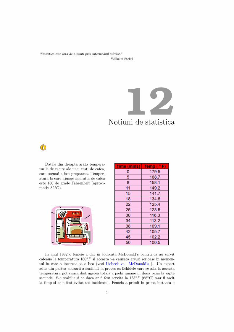
Datele din dreapta arata tempera-turile de racire ale unei cesti de cafea,care tocmai a fost preparata. Temper-atura la care ajunge aparatul de cafeaeste 180 de grade Fahrenheit (aproxi-mativ 82∘𝐶).

In anul 1992 o femeie a dat in judecata McDonald’s pentru ca au servitcafeaua la temperatura 180∘𝐹 si aceasta i-a cauzata arsuri serioase in momen-tul in care a incercat sa o bea (vezi Liebeck vs. McDonald’s ). Un expertadus din partea acuzarii a sustinut la proces ca lichidele care se afla la aceastatemperatura pot cauza distrugerea totala a pielii umane in doua pana la saptesecunde. S-a stabilit si ca daca ar fi fost servita la 155∘𝐹 (68∘𝐶) s-ar fi racitla timp si ar fi fost evitat tot incidentul. Femeia a primit in prima instanta o

1

despagubire de 2.7 milioane de dolari. Ca urmare a acestui caz faimos multerestaurante servesc acum cafeaua la o temperatura de aproximativ 155∘𝐹 . Catde mult ar trebui sa astepte restaurantele din momentul in care cafeaua este tur-nata in ceasca din aparat si pana cand ea poate fi servita, pentru a se asiguraca nu este mai fierbinte de 155∘𝐹 ?

∙ Determinati ecuatia unui model de regresie exponentiala pentru a reprezentadatele

∙ Reprezentati grafic curba obtinuta∙ Decideti daca ecuatia obtinuta este buna pentru a reprezenta datele exis-

tente in tabel∙ Interpolare: Cand ajunge temperatura cafelei la 106∘𝐹 ?∙ Extrapolare: Care este temperatura prezisa, de modelul gasit, peste o ora?

2

Notiuni teoretice:

∙ Statistica descriptiva: populatie statistica, esantion statistic, serie sta-tistica, frecventa abosluta, frecventa relativa, histograma, media ��, mediana𝑚3, amplitudinea 𝐴, dispersia 𝜎2, deviatia standard 𝜎, moda (modulul) 𝑚𝑜,dispersia de selectie 𝑠2, deviatia standard de selectie 𝑠, cuartilele 𝑄1, 𝑄2, 𝑄3,indicatorul de asimetrie 𝑠𝑘 (skewness), indicatorul de aplatizare 𝑘 (kurtosis)

Intervale de incredere

∙ confidence intervals are used when we want to estimate a population pa-rameter from a sample. The parameter may be estimated by a single value (apoint estimate) but it is usually preferable to estimate it by an interval whichwill give some indication of the amount of uncertainty attached to the estimate.

∙ the common notation for the parameter in question is 𝜃. Often, thisparameter is the population mean 𝜇 , which is estimated through the samplemean ��.

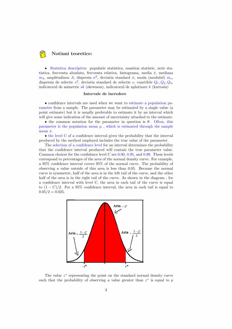
∙ the level C of a confidence interval gives the probability that the intervalproduced by the method employed includes the true value of the parameter.

The selection of a confidence level for an interval determines the probabilitythat the confidence interval produced will contain the true parameter value.Common choices for the confidence level C are 0.90, 0.95, and 0.99. These levelscorrespond to percentages of the area of the normal density curve. For example,a 95% confidence interval covers 95% of the normal curve. The probability ofobserving a value outside of this area is less than 0.05. Because the normalcurve is symmetric, half of the area is in the left tail of the curve, and the otherhalf of the area is in the right tail of the curve. As shown in the diagram , fora confidence interval with level C, the area in each tail of the curve is equalto (1 − 𝐶)/2. For a 95% confidence interval, the area in each tail is equal to0.05/2 = 0.025.

The value 𝑧* representing the point on the standard normal density curvesuch that the probability of observing a value greater than 𝑧* is equal to 𝑝

3

is known as the upper 𝑝 critical value of the standard normal distribution.For example, if 𝑝 = 0.025, the value 𝑧* such that 𝑃 (𝑍 > 𝑧*) = 0.025, or𝑃 (𝑍 < 𝑧*) = 0.975, is equal to 1.96. For a confidence interval with level C, thevalue 𝑝 is equal to (1−𝐶)/2. A 95% confidence interval for the standard normaldistribution is then the interval (−1.96, 1.96), since 95% of the area under thecurve falls within this interval.

Medie necunoscuta si deviatie standard cunoscuta

Teorema:Pentru o populatie cu media 𝜇 necunoscuta si deviatie standard 𝜎 cunos-

cuta, un interval de incredere pentru media populatiei, construit pe baza unuiesantion de volum 𝑛, este:

(��− 𝑧*𝜎√𝑛, �� + 𝑧*

𝜎√𝑛

)

unde 𝑧* este valoarea critica corespunzatoare lui1 − 𝐶

2pentru distributia nor-

mala standard, adica 𝑧* = Φ( 1−𝐶2 ).

Medie necunoscuta si deviatie standard necunoscuta

∙ cand deviatia standard 𝜎 este necunoscuta este estimata de obicei prin 𝑠numita eroarea standard /deviatia standard de selectie , unde:

𝑠2 =

𝑛∑𝑖=1

(𝑥𝑖 − ��)2

𝑛− 1

si 𝑛 este volumul selectiei.Teorema:Pentru o populatie cu media necunoscuta 𝜇 si deviatia standard 𝜎 necunos-

cuta, un inteval de incredere pentru media populatiei, construit pe baza unuiesantion de volum 𝑛, este:

(��− 𝑡*𝑠√𝑛, �� + 𝑡*

𝑠√𝑛

)

unde 𝑡* este valoarea critica corespunzatoare lui1 − 𝐶

2pentru distributia

𝑡-Student cu n-1 grade de libertate.∙ Pasul final consta in interpretarea rezultatului: pe baza datelor avute

suntem 𝐶% siguri ca adevarata medie a populatiei se afla intre valorile date deintervalul gasit

∙ valorile critice 𝑧* si 𝑡* se pot gasi in tabelul urmator z-t-table∙ distributia 𝑡 sau distributia Student este data de catre urmatoarea

densitate de probabilitate:

𝑓(𝑡) =Γ(𝑛+1

2 )√𝑛𝜋Γ(𝑛

2 )

(1 +

𝑡2

𝑛

)−𝑛+12

De retinut

4

unde 𝑛 este numarul de grade de libertate si Γ este functia lui Euler.

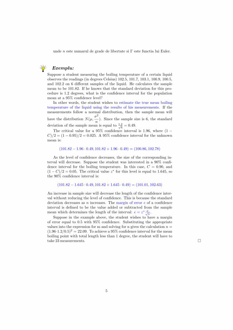
Suppose a student measuring the boiling temperature of a certain liquidobserves the readings (in degrees Celsius) 102.5, 101.7, 103.1, 100.9, 100.5,and 102.2 on 6 different samples of the liquid. He calculates the samplemean to be 101.82. If he knows that the standard deviation for this pro-cedure is 1.2 degrees, what is the confidence interval for the populationmean at a 95% confidence level?

In other words, the student wishes to estimate the true mean boilingtemperature of the liquid using the results of his measurements. If themeasurements follow a normal distribution, then the sample mean will

have the distribution 𝑁(𝜇,𝜎2

𝑛). Since the sample size is 6, the standard

deviation of the sample mean is equal to 1.2√6

= 0.49.

The critical value for a 95% confidence interval is 1.96, where (1 −𝐶)/2 = (1 − 0.95)/2 = 0.025. A 95% confidence interval for the unknownmean is:

(101.82 − 1.96 · 0.49, 101.82 + 1.96 · 0.49) = (100.86, 102.78)

As the level of confidence decreases, the size of the corresponding in-terval will decrease. Suppose the student was interested in a 90% confi-dence interval for the boiling temperature. In this case, 𝐶 = 0.90, and(1 − 𝐶)/2 = 0.05. The critical value 𝑧* for this level is equal to 1.645, sothe 90% confidence interval is:

(101.82 − 1.645 · 0.49, 101.82 + 1.645 · 0.49) = (101.01, 102.63)

An increase in sample size will decrease the length of the confidence inter-val without reducing the level of confidence. This is because the standarddeviation decreases as 𝑛 increases. The margin of error 𝑒 of a confidenceinterval is defined to be the value added or subtracted from the samplemean which determines the length of the interval: 𝑒 = 𝑧* 𝜎√

𝑛.

Suppose in the example above, the student wishes to have a marginof error equal to 0.5 with 95% confidence. Substituting the appropriatevalues into the expression for m and solving for n gives the calculation 𝑛 =(1.96·1.2/0.5)2 = 22.09. To achieve a 95% confidence interval for the meanboiling point with total length less than 1 degree, the student will have totake 23 measurements. �

Exemplu:

5

Testarea ipotezelor statistice

In a decision-making process managers make hypotheses which afterwardscan be tested using the tools of statistics. A hypothesis test examines twoopposing hypotheses about a population: the null hypothesis and the alternativehypothesis. How you set up these hypotheses depends on what you are tryingto show.

Null hypothesis 𝐻0

∙ the null hypothesis states that a population parameter is equal to a value.The null hypothesis is often an initial claim that managers specify using previousresearch or knowledge.

Alternative Hypothesis 𝐻𝑎

∙ the alternative hypothesis states that the population parameter is differ-ent than the value of the population parameter in the null hypothesis. Thealternative hypothesis is what you might believe to be true or hope to provetrue.

What are some common hypotheses?E.g.: Hypothesis to determine whether a population mean 𝜇, is equal to

some target value 𝜇0 include the following:

⇒ for a big sample size 𝑛 or 𝜎known

· we use the z test and compute:

𝑧𝑐𝑎𝑙𝑐 =��− 𝜇0

𝜎√𝑛

⇒ for a sample size 𝑛 < 30 and 𝜎unknown

· we use the 𝑡 test and compute:

𝑡𝑐𝑎𝑙𝑐 =��− 𝜇0

𝑠√𝑛

Two-tailed test:

𝐻0 : 𝜇 = 𝜇0

𝐻𝑎 : 𝜇 = 𝜇0

⇒ the critical region/ region of rejection, when we reject 𝐻0 is given by:

𝑧𝑐𝑎𝑙𝑐 < −𝑧*𝛼2or 𝑧𝑐𝑎𝑙𝑐 > 𝑧*𝛼

2𝑡𝑐𝑎𝑙𝑐 < −𝑡*𝛼

2 ,𝑛−1 or 𝑡𝑐𝑎𝑙𝑐 > 𝑡*𝛼2 ,𝑛−1

Upper-tailed test:

𝐻0 : 𝜇 = 𝜇0

𝐻𝑎 : 𝜇 > 𝜇0

⇒ the critical region/ region of rejection, when we reject 𝐻0 is given by:

6

𝑧𝑐𝑎𝑙𝑐 > 𝑧*𝛼 𝑡𝑐𝑎𝑙𝑐 > 𝑡*𝛼,𝑛−1

Lower-tailed test:

𝐻0 : 𝜇 = 𝜇0

𝐻𝑎 : 𝜇 < 𝜇0

⇒ the critical region/ region of rejection, when we reject 𝐻0 is given by:

𝑧𝑐𝑎𝑙𝑐 < −𝑧*𝛼 𝑡𝑐𝑎𝑙𝑐 < −𝑡*𝛼,𝑛−1

⇒ in all these examples 𝛼 is the significance level corresponding to a confi-dence level 𝐶 = 1 − 𝛼

⇒ the critical values 𝑧* and 𝑡* for different confidence intervals are shownin the z-t-table

Estimarea parametrilor prin metoda momentelor

The method of moments is a method of estimation of population parameters.The method is based on the assumption that the sample moments are goodestimates of the corresponding population moments.

∙ for a population 𝑋 the moments 𝜇𝑘 (or 𝑀𝑘) of order 𝑘 are defined as:

𝜇𝑘 = 𝑀(𝑋𝑘) =

⎧⎪⎪⎪⎪⎪⎪⎨⎪⎪⎪⎪⎪⎪⎩

∞∫−∞

𝑥𝑘𝑓(𝑥)𝑑𝑥, if 𝑋 is continuous

∑𝑖∈𝐼

𝑥𝑘𝑖 𝑝𝑖, if 𝑋 is discrete

∙ the sample moment 𝑚𝑘 of order 𝑘 of a sample of size 𝑛 is defined as:

𝑚𝑘 =1

𝑛

𝑛∑𝑖=1

𝑋𝑘𝑖

The method of moments estimation simply equates the moments of the dis-tribution with the sample moments 𝜇𝑘 = 𝑚𝑘 and solves for the unknown pa-rameters. (the distribution must have finite moments)

Method of moments:

1. we want to estimate a parameter 𝜃

2. calculate low-order moments 𝜇𝑘 as functions of 𝜃

3. set up a system of equations setting the population moments 𝜇𝑘 equalto the sample moments 𝑚𝑘, and derive expressions for the parameter asfunctions of the sample moments 𝑚𝑘.

7

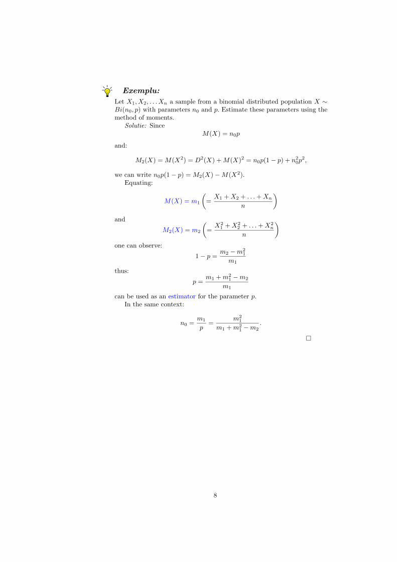
Let 𝑋1, 𝑋2, . . . 𝑋𝑛 a sample from a binomial distributed population 𝑋 ∼𝐵𝑖(𝑛0, 𝑝) with parameters 𝑛0 and 𝑝. Estimate these parameters using themethod of moments.

Solutie: Since𝑀(𝑋) = 𝑛0𝑝

and:

𝑀2(𝑋) = 𝑀(𝑋2) = 𝐷2(𝑋) + 𝑀(𝑋)2 = 𝑛0𝑝(1 − 𝑝) + 𝑛20𝑝

2,

we can write 𝑛0𝑝(1 − 𝑝) = 𝑀2(𝑋) −𝑀(𝑋2).Equating:

𝑀(𝑋) = 𝑚1

(=

𝑋1 + 𝑋2 + . . . + 𝑋𝑛

𝑛

)and

𝑀2(𝑋) = 𝑚2

(=

𝑋21 + 𝑋2

2 + . . . + 𝑋2𝑛

𝑛

)one can observe:

1 − 𝑝 =𝑚2 −𝑚2

1

𝑚1

thus:

𝑝 =𝑚1 + 𝑚2

1 −𝑚2

𝑚1

can be used as an estimator for the parameter 𝑝.In the same context:

𝑛0 =𝑚1

𝑝=

𝑚21

𝑚1 + 𝑚21 −𝑚2

.

�

Exemplu:

8

Analiza regresiva prin metoda celor mai mici patrate

∙ in sectiunile anterioare am considerat experimente pentru care am observato singura cantitate (variabila) aleatoare, iar esantioanele respective au constatdin date reprezentate de numere reale 𝑥1, 𝑥2, . . . , 𝑥𝑛

∙ in aceasta sectiune vom considera experimente ın care suntem interesati dedoua cantitati (variabile) aleatoare, deci esantioanele respective vor fi reprezen-tate de perechi de numere reale (𝑥1, 𝑦1), (𝑥2, 𝑦2), . . . , (𝑥𝑛, 𝑦𝑛)

∙ in analiza regresiva una din cele doua variabile (spre exemplu 𝑋) esteprivita ca o variabila ce poate fi masurata (determinata) cu precizie, numitavariabila independenta si suntem interesati de modul cum cealalta variabila𝑌 (numita variabila dependenta) depinde de aceasta: spre exemplu sunteminteresati de modul de aportul de crestere 𝑌 al animalelor ın functie de cantitateazilnica de hrana 𝑋.

∙ in general, intr-un anumit experiment alegem valorile 𝑥1, 𝑥2, . . . , 𝑥𝑛 apoiobservam valorile 𝑦1, 𝑦2, . . . , 𝑦𝑛 ale unei variabile aleatoare 𝑌 , obtinand astfelun esantion (𝑥1, 𝑦1), (𝑥2, 𝑦2), . . . , (𝑥𝑛, 𝑦𝑛)

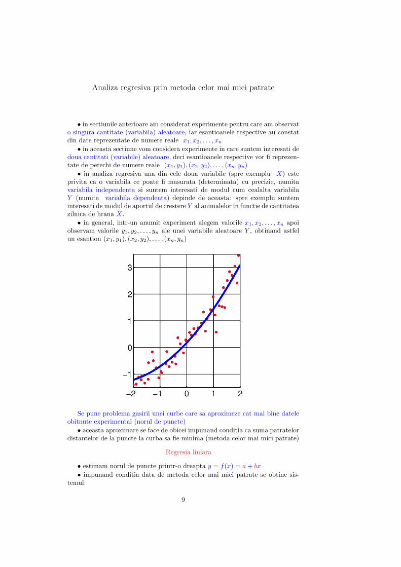
Se pune problema gasirii unei curbe care sa aproximeze cat mai bine dateleobitnute experimental (norul de puncte)

∙ aceasta aproximare se face de obicei impunand conditia ca suma patratelordistantelor de la puncte la curba sa fie minima (metoda celor mai mici patrate)

Regresia liniara

∙ estimam norul de puncte printr-o dreapta 𝑦 = 𝑓(𝑥) = 𝑎 + 𝑏𝑥

∙ impunand conditia data de metoda celor mai mici patrate se obtine sis-temul:

9

{𝑎 + 𝑏 ·

∑𝑛𝑖=1 𝑥𝑖

𝑛 =∑𝑛

𝑖=1 𝑦𝑖

𝑛

𝑎 ·∑𝑛

𝑖=1 𝑥𝑖

𝑛 + 𝑏 ·∑𝑛

𝑖=1 𝑥2𝑖

𝑛 =∑𝑛

𝑖=1 𝑥𝑖𝑦𝑖

𝑛

care are solutia:

𝑏 =𝑛∑

𝑥𝑦 −∑

𝑥 ·∑

𝑦

𝑛∑

𝑥2 − (∑

𝑥)2

si:

𝑎 =

∑𝑛𝑖=1 𝑦𝑖𝑛

− 𝑏

∑𝑛𝑖=1 𝑥𝑖

𝑛= 𝑌 − 𝑏��.

Regresia parabolica

∙ estimam norul de puncte printr-o parabola 𝑦 = 𝑓(𝑥) = 𝑎 + 𝑏𝑥 + 𝑐𝑥2

∙ impunand conditia data de metoda celor mai mici patrate se obtine sis-temul: ⎧⎪⎨⎪⎩

𝑎 · 𝑛 + 𝑏 ·∑

𝑥 + 𝑐 ·∑

𝑥2 =∑

𝑦

𝑎 ·∑

𝑥 + 𝑏 ·∑

𝑥2 + 𝑐 ·∑

𝑥3 =∑

𝑥𝑦

𝑎 ·∑

𝑥2 + 𝑏 ·∑

𝑥3 + 𝑐 ·∑

𝑥4 =∑

𝑥2𝑦

Regresia hiperabolica

∙ estimam norul de puncte printr-o hiperbola 𝑦 = 𝑓(𝑥) = 𝑎 + 𝑏𝑥

∙ impunand conditia data de metoda celor mai mici patrate se obtine sis-temul: {

𝑎 · 𝑛 + 𝑏 ·∑

1𝑥 =

∑𝑦

𝑎 ·∑

1𝑥 + 𝑏 ·

∑1𝑥2 =

∑ 𝑦𝑥

Regresia exponentiala

∙ estimam norul de puncte printr curba 𝑦 = 𝑓(𝑥) = 𝑎 · 𝑏𝑥∙ se logaritmeaza relatia si obtinem:

ln 𝑦 = ln 𝑎 + ln 𝑏 · 𝑥

care are forma unui model de regresie liniara pentru datele (𝑥𝑖, ln 𝑦𝑖), 𝑖 = 1, 𝑛deci 𝑎 si 𝑏 se determina din:

ln 𝑏 =𝑛∑

𝑥 ln 𝑦 −∑

𝑥 ·∑

ln 𝑦

𝑛∑

𝑥2 − (∑

𝑥)2

si:

ln 𝑎 =

∑𝑛𝑖=1 ln 𝑦𝑖𝑛

− ln 𝑏 ·∑𝑛

𝑖=1 𝑥𝑖

𝑛.

prin intermediul formulelor 𝑎 = 𝑒ln 𝑎 si 𝑏 = 𝑒ln 𝑏

10

Probleme rezolvate

Problema 1. Calculati cuartilele 𝑄1, 𝑄2, 𝑄3 pentru urmatoarea seriestatistica simpla

𝑋 : 1, 2, 5, 7, 11, 21, 22, 23, 29

si abaterea cuartilica.

Solutie: Facem mai ıntai observatia ca mediana 𝑚𝑒 coincide cu cuartila 𝑄2.Deoarece seria statistica data are un numar impar de termeni (9 mai exact),

vom folosi formula corespunzatoare pentru a determina cuartila 𝑄2 si avem

𝑥 9+12

= 𝑥5 = 11 ⇒ 𝑚𝑒 = 𝑄2 = 11.

Mai departe pentru a determina prima cuartila tinem cont de seria statisticasimpla

1, 2, 5, 7, 11

care are tot un numar impar de termeni si obtinem

𝑥 5+12

= 𝑥3 = 5 ⇒ 𝑄1 = 5.

Analog procedam pentru a treia cuartila tinand cont de seria statisticasimpla

11, 21, 22, 23, 29

care are tot un numar impar de termeni si rezulta

𝑥 5+12

= 𝑥3 = 22 ⇒ 𝑄3 = 22.

Atunci rezulta ca abaterea cuartilica este

𝑄 = 𝑄3 −𝑄1 = 22 − 5 = 17.

Problema 2. Fie seria statistica

𝑋 : 1, 5, 4, 20, 3, 16.

Determinati:a) amplitudinea absoluta 𝐴.b) abaterea medie patratica �� (𝑋).c) dispersia 𝜎2 (𝑋).d) deviatia standard 𝜎 (𝑋).e) coeficientul de variatie 𝑐𝑣(𝑋).

Solutie: a) Amplitudinea absoluta 𝐴 este

𝐴 = 𝑋max −𝑋min = 20 − 1 = 19.

11

b) Abaterea medie patratica �� (𝑋) se obtine astfel

𝑎 (𝑋) =|1 − 𝑥| + |5 − 𝑥| + |4 − 𝑥| + |20 − 𝑥| + |3 − 𝑥| + |16 − 𝑥|

6,

unde media 𝑥 este

𝑥 =1 + 5 + 4 + 20 + 3 + 16

6= 8, 16.

Atunci rezulta�� (𝑋) ≃ 6, 55.

c) Dispersia este

𝜎2 (𝑋) =1

6

6∑𝑖=1

(𝑥𝑖 − 𝑥)2

=

=1

6

(7, 162 + 3, 162 + 4, 162 + 11, 842 + 5, 162 + 7, 842

)= 51, 138 ≃ 51.

d) deviatia standard rezulta imediat de mai sus

𝜎 (𝑋) =√𝜎2(𝑋) =

√51 = 7, 14 ≃ 7.

e) Din cele de mai sus, rezulta coeficientul de variatie

𝑐𝑣(𝑋) =𝜎 (𝑋)

𝑥· 100 = 85, 78.

Problema 3. Pe o perioada de mai multi ani, un profesor a ınregistratrezultatele elevilor si a obtinut ca media 𝜇 a acestor rezultate este 72 siabaterea standard 𝜎 = 12. Clasa de 36 de elevi pe care-i ınvata ın prezentare o medie 𝑥 = 75, 2, iar profesorul afirma ca ea este superioara celorde pana acum. Intrebarea care se pune este daca media clasei 𝑥 este unargument suficient pentru a sustine afirmatia profesorului la un nivelulde semnificatie dat 𝛼 = 0, 05 (95% sigur).

Solutie: Etapa 1: Formularea ipotezei nule 𝐻0

𝐻0 : 𝑥 = 𝜇 = 72 ⇔ clasa nu este superioara.

Etapa 2: Formularea ipotezei alternative 𝐻𝑎

𝐻𝑎 : 𝑥 = 𝜇 > 72 ⇔ clasa este superioara.

Etapa 3: Metodologia de verificare a ipotezelora) Cand ın ipoteza nula media populatiei si deviatia standard sunt cunos-

cute, atunci folosim scorul standard 𝑧 ca si test statistic.b) Nivelul de semnificatie este dat si este 𝛼 = 0, 05.

c) In baza teoremei limita centrala distributia mediilor esantioanelor esteaproape normala, deci prin urmare distributia normala va fi folosita pentru

12

determinarea regiunii critice. Regiunea critica este egala cu multimea valorilorscorului standard 𝑧 care determina respingerea ipotezei nule si este situata laextremitatea dreapta a distributiei normale. Regiunea critica este la dreaptadeoarece valori mari ale mediei esantionului sustin ipoteza alternativa ın timpce valori apropiate valorii 72 sustin ipoteza nula.

Valoarea critica ce desparte zona valorilor ”nu este superior”de zona valorilor”este superior”este determinata de probabilitatea 𝛼 = 0, 05 de a comite o eroarede tip 𝐼 (eroarea de tip 𝐼 apare cand ipoteza nula este adevarata si tot ea esterespinsa).

Etapa 4: Determinarea valorii testului statisticValoarea testului statistic este data de formula

𝑧𝑐𝑎𝑙𝑐 =𝑥− 𝜇𝜎√𝑛

=75, 2 − 72

12√36

= 1, 6.

Etapa 5: Luarea unei decizii si interpretarea eiDaca comparam valoarea gasita cu valoarea critica observam ca:

1, 6 < 1, 65

Conform celor stabilite in sectiunea ipotezelor statistice respingem ipoteza 𝐻0

daca:𝑧𝑐𝑎𝑙𝑐 > 𝑧*𝛼

Decizia: nu putem respinge ipoteza nula !In final, tragem concluzia ca probele nu sunt suficiente pentru a sustine ca

actuala clasa este superioara celor anterioare.

Problema 4. Noua dintre studentii unei facultati cu profil sportiv au fostselectati pentru a da un test de alergare pe distanta mare. Masuratorilepentru acest grup au condus la un timp mediu de 12, 87 minute cu oabatere standard 𝑠 = 1, 3. Sa se aproximeze, cu o probabilitate de 90%,timpul mediu pe care studentii intregii facultati il vor inregistra pe aceadistanta .

Solutie: Deoarece nu se cunoaste dispersia populatiei iar esantionul are volu-mul mai mic dacat 30, intervalul de ıncredere este dat de formula(

𝑥− 𝑠√𝑛𝑡𝑛−1,𝛼2

, 𝑥 +𝑠√𝑛𝑡𝑛−1,𝛼2

),

unde 𝑥 = 12, 87 ; 𝑠 = 1, 3 ; 𝑛 = 9 ; 𝛼 = 0, 10 ; iar 𝑡𝑛−1,𝛼2este valoarea critica a

repartitiei Student (statisticianul William Sealy Gosset folosea acest pseudonim

in articolele sale ) cu 𝑛−1 grade de libertate corespunzatoare valorii𝛼

2=

1 − 𝐶

2care ın cazul nostru este 𝑡9−1, 0.05 = 𝑡8, 0,05 = 1, 860 conform tabelului z-t-table

Obtinem intervalul(12.064, 13.676)

In concluzie suntem 90% siguri ca timpul mediu inregistrat de un studentpe acea distanta va fi in acest interval !

13

Probleme propuse

Problema 1. Fiind date seriile statistice simple

𝑋 : 1, 5, 7, 8, 10,

𝑌 : 1, 6, 100, 135

determinati mediana ın ambele cazuri.

Problema 2. Intr-o colectivitate s-au ales date statistice numerice obtinandu-se

𝑋 : 4, 1, 1, 5, 6, 3, 2, 1,

𝑌 : 100, 90, 40, 80, 70, 50, 100, 70.

Aflati dupa care din variabilele de mai sus, colectivitatea este mai omogena.

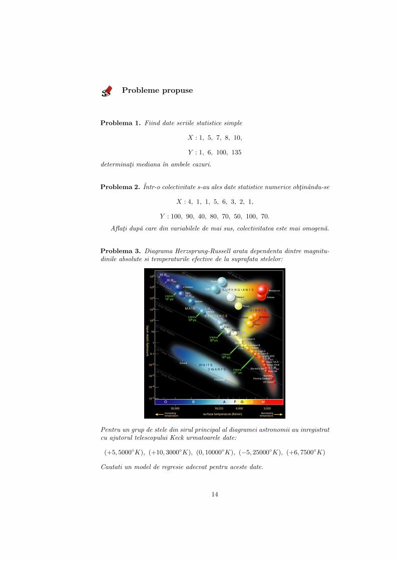
Problema 3. Diagrama Herzsprung-Russell arata dependenta dintre magnitu-dinile absolute si temperaturile efective de la suprafata stelelor:

Pentru un grup de stele din sirul principal al diagramei astronomii au inregistratcu ajutorul telescopului Keck urmatoarele date:

(+5, 5000∘𝐾), (+10, 3000∘𝐾), (0, 10000∘𝐾), (−5, 25000∘𝐾), (+6, 7500∘𝐾)

Cautati un model de regresie adecvat pentru aceste date.

14

Problema 4. The operations manager of a large production plant would like toestimate the mean amount of time a worker takes to assemble a new electroniccomponent. Assume that the standard deviation of this assembly time is 3.6minutes.

a) After observing 120 workers assembling similar devices, the manager no-ticed that their average time was 16.2 minutes. Construct a 95% confidenceinterval for the mean assembly time.

b) How many workers should be involved in this study in order to have themean assembly time estimated up to ±15 seconds with 95% confidence?

Problema 5. In order to ensure efficient usage of a server, it is necessaryto estimate the mean number of concurrent users. According to records, thesample mean and sample standard deviation of number of concurrent users at100 randomly selected times is 37.7 and 9.2, respectively.

Construct a 90% confidence interval for the mean number of concurrentusers.

Problema 6. Let 𝑋1, 𝑋2, ..., 𝑋𝑛 be normal random variables with mean 𝑚 andvariance 𝜎2. What are the method of moments estimators of the mean 𝑚 andvariance 𝜎2?

Problema 7. A consumer group, concerned about the mean fat content of acertain steakburger submits to an independent laboratory a random sample of 12steakburgers for analysis. The percentage of fat in each of the steakburgers is asfollows:

21 18 19 16 18 24 22 19 24 14 18 15

The manufacturer claims that the mean fat content of this steakburger is around20%. Assuming percentage fat content to be normally distributed with a standarddeviation of 3, carry out a hypothesis test, with significance level 𝛼 = 0.05, inorder to advise the comsumer group as to the validity of manufacturer’s claim.

Problema 8. During a particular week, 13 babies were born in a maternityunit. Part of the standard procedure is to measure the length of the baby. Givenbelow is a list of the lengths, in centimetres, of the babies born in this particularweek.

49 50 45 51 47 49 48 54 53 55 45 50 48

Assuming that this sample came from an underlying normal population, test, atthe 5% significance level, the hypothesis that the population mean length is 50cm.

Problema 9. 𝑋1, 𝑋2, . . . 𝑋𝑛 represents a selection from a population 𝑋 withexponential distribution, i.e. the probability density function is:

𝑓(𝑥) =

{𝜆𝑒−𝜆𝑥, if 𝑥 ≥ 0,

0, otherwise

Estimate the parameter 𝜆 using the method of moments.

Problema 10. 𝑋1, 𝑋2, . . . 𝑋𝑛 represents a selection from a population 𝑋 withPoisson distribution, i.e. the probability mass function is:

𝑃 (𝑋 = 𝑘) =

{𝑒−𝜆 𝜆𝑘

𝑘! , if 𝑘 = 0, 1, . . .

0, otherwise

15

Estimate the parameter 𝜆 using the method of moments.

16