


![Corina NAFORNIŢĂ · 2005-04-14 · web, to prevent commercial use of such images. One example of visible watermarking has been implemented by IBM for the Vatican library [BMM96].](https://static.fdocumente.com/doc/165x107/5e3588d6cadfde3f845ccc7a/corina-naforni-2005-04-14-web-to-prevent-commercial-use-of-such-images-one.jpg)

Limbile
Pagini
Legal

1Institutul Naţional de Studii şi Cercetări pentru Comunicaţii, Bucureşti, România
Utilizarea tehnologiilor multimodale pentru proiectarea de
sisteme de securitate (II): Procesul de învăţare, clasificarea
datelor şi evaluarea performanţelor
The Multimodal Technologies usage for Security Systems Design
(II): Learning process, data classification and performance
evaluation
Sorin Soviany1, Sorin Puşcoci1
Rezumat: Tehnologiile multimodale constau în metode şi algoritmi de procesare a datelor din
surse multiple şi, de regulă, independente, ca bază pentru generarea şi furnizarea de informaţii
relevante (de tip scor) pentru funcţii de decizie în variate aplicaţii. Tehnologiile multimodale
asigură suportul informaţional pentru sistemele de decizie, în acest caz pentru cele din domeniul
securităţii datelor şi reţelelor. Principiile şi instrumentele pentru proiectarea de sisteme de
securitate bazate pe tehnologii multimodale au în vedere aspecte relevante pentru optimizarea
funcţiilor de securitate în vederea atingerii unor performanţe adaptate cerinţelor utilizatorilor
aplicaţiilor reale. Instrumentele de proiectare se bazează pe tehnici specifice din domeniul
inteligenţei artificiale, în particular din cel al învăţării maşină. Măsurile de performanţă pentru
caracterizarea securităţii şi eficienţei sistemelor multimodale sunt definite în lucrare, având în
vedere importanţa practică a acestora.
Cuvinte cheie: tehnologii multimodale, învăţare maşină
Abstract: The multimodal technologies include methods and algorithms that are applied to
process data from multiple and, typically, independent sources, as support to generate and
provide meaningful infoprmation (such as scoring) for decisions functions in various
applications. The multimodal technologies provide the information support to the decision
systems, in this case with focus on data and networks security. The principles and tools for the
multimodal security systems design concern relevant issues for the security functions
optimization in order to reach the required performances customized for the real applications
end-users. The design tools are based on Artificial Inteligence (AI) area specific techniques,
particularly on Machine Learning (ML). The performance amounts for the multimodal systems
security and efectiveness assessment are defined in the paper, given their practical utility.
Keywords: multimodal technologies, machine learning
1. Introduction
A modern approach for the security systems design and development is based on the multimodal
technologies. These technologies include algorithms that are designed to process data from

multiple and independent sources, outcoming meaningful information (such as scoring) for
decision making in various applications including those from data and networks security domain.
The design and development of security functions based on multiple factors, with various data
types processing, has significant challenges concerning the complexity and performances
adjustment even for conventional desktop-based applications [1]. The principles and tools for the
multimodal security systems design concern relevant issues for the security functions
optimization in order to reach the required performances customized for the real applications
end-users. The design tools are based on Artificial Inteligence (AI) area specific techniques,
particularly on Machine Learning (ML). The core functionality is represented by the learning
process together with some optimizations tools and methods that are used in order to provide
high-performance solutions for the real applications.
The paper has the following structure: Section 2, that presents the learning process and modeling
principles, also with a bried presentation of the typical data fusion rules; Section 3, that presents
the typical performance measures for the multimodal security systems; Section 4, that concludes
this paper.
2. The learning process/modeling, optimization and data fusion
The multimodal security systems design requires to perform a learning process based on
relevant data in order to develop a high-performance solution that should meet the real security
application requirements. Typically a supervised lerarning process is implemented for biometric
applications, but other applications like intrusion detection (IDS, Intrusion Detection Systems)
require to develop a combination of supervised and unsupervised models, such as to provide a
reliable outliers or anomalies detection before the supervised learning. In the remainder of the
paper only the supervised learning (data classification) is considered, together with:
optimizations methods: starting from the various available models for data classification
(supervised learning) that could be applied in order to provide specific security decisions,
some particular design options may be considered in order to enhance the overall learning
process performance, such as:
Moving from multi-class to binary classification;
Target-vs.-non-target classification, sometimes within a hierarchical classifier (with
multi-stage decisions) for multi-level security systems;
data fusion rules, at several processing stage. The data fusion is the core functionality for
any security system in which several data types should be integrated within the multimodal
approach.
2.1 Data classification process
The data classification process in multimodal security systems is performed with 2
complementary approaches [1]:
the statistical approach with supervised learning, in which the processing output is an
estimator of the posterior probability for the class membership or, depending on the applied
model structure, the distance to a decision boundary. This value is computed or estimated
using a classifier’s discriminant function;
the deterministic approach with distances computation and matching score, in which the
similarity degree is evaluated between a current pattern and a reference one (both of them
being represented as feature vectors), using a point-to-point comparison (or, if case, with a
distance estimation).
2.1.1 The supervised learning for data classification [1]
The supervised learning uses classification models that are varying depending on the following
criteria [1],[2],[3],[4],[5],[6]:
the features representation or combination modality, criterion according to which the
available classifiers are grouped in 2 categories [2]:
linear classifiers, in which the decision is based on a classifier output that is computed
using a linear combination of the input features;
non-linear classifiers, that generate class membership decisions using non-linear
combinations of the input features;
the classifiers parameters and hyper-parameters evaluation modality, that differentiates the
classifiers into ther following categories [2],[4],[5]:
generative classification models, that directly uses class-conditioned probability
density functions ( ( | )p x Class where x is the input feature vector and Class is the
class label of the current sample). The decision rule derives from Bayes theorem
application, leading to models that are different depending on the relationships
between the class covariance matrices and some specific parameterizations. Actually
the generative models differ according to the parameterization degree [4]:
o generative classifiers with parametric models, in which the underlying models
(typically Gaussians) design uses statistical parameters including class means
and variances (covariances), for Gaussian class distributions. The Gaussian
parametric models-based classifiers are NMC (the Nearest Mean Classifier),
LDC (the Linear Discriminant Classifier), QDC (the Quadratic Discriminant
Classifier with normal densities), GMM (Gaussian Mixture Models);
o non-parametric generative classifiers, that do not use explicitly parameterized
models with statistical estimates of the input data. The non-parametric
classifiers are the Parzen classifier and the Naive-Bayes classifier. Actually a
certain parameterization still remains (related to the underlying model
mathematical structure), but these parameters do not represent statistical
properties of the input samples (statistics from the class distributions);
discriminative classification models, that uses direct discrimination rules in ordet to
maximize the output quality on a training datset. The discriminative classifiers directly
model the class posterior probabilities or the decision function, without the explicit
usage of per-class probability density functions estimates. The discrimination criterion
allows to distinguish between 2 types of classification models:
o distance-based discriminative classifiers, in which the discriminant estimation is
done using a distance measure. The most common distance-based classifiers are
the Fisher classifier, the logistic classifier, the KNN classifier (K-Nearest
Neighbors decision rule), the SVM (Support Vector Machines) classifier;
o discriminative classifiers for the error minimization performs the discrimination
function using an optimal criterion for the error rate minimization. The most
common classifiers based on discrimination for error minimization are: the
perceptron, the multi-layer neural networks and the decision tree;
the classes number separates 2 types of classifiers:
binary classifiers, that only discriminates between 2 classes;
multi-class classifiers, in which the separation is among more than 2 classes.
2.1.2 The matching (similarity) score computing for data classification [1]
The deterministic approach using matching or similarity scores computes a distance measure
within the feature vector space; the distance is evaluated between the current pattern and a
reference sample that was previously enrolled. This approach is typically applied for many
biometric systems in which the design is based on the comparison between the current biometric
sample applied to the system input and one or several biometric templates retrieved from the
system database.
This approach proceeds to compute the similarity score S0 between the current feature vector x
and the reference y using a certain distance. The procedure requires the following steps:
the distance computation ( , )d x y . The typical distances for this computational process are
Euclidian distance and Mahalanobis distance [5],[7]:
the Euclidian distance is commonly used to compute a distance-based score within the
input feature space. For 2 vectors x and y with the same size D, the Euclidian distance
is computed as follows:
2
1
( , ) [ ] [ ]D
E
i
d x y x i y i
(1)
the Mahalanobis distance is a distance based on the correlation among variables and
can be used to evaluate the similarity degree among 2 variables sets. Its definition for 2
vectors x and y with the same size D is the following:
1( , )T
Md x y x y x y (2)
where is the covariance matrix of the 2 feature vectors, computed as
( , ) [ ] [ ]T
Cov x y E x E x y E y
(3)
[] is the operator that provides the mean of a random variable. For a binary
classification problem (such as the biometric verification with authentic vs. impostor
discrimination or the fraudulent actions detection with genuine vs. attack
discrimination), the covariance matrix is typically computed with the following
equation [5]:
1 1 1 2(1 )P P (4)
in which 1 and
2 are the covariance matrices for the 2 classes, and the weights are
their priors. The 1st class is usually the target class for the application. The
Mahalanobis distance has 2 properties that make it a very useful similarity criterion
[8]:
o exploiting the existing correlation among the features. This property support
some additional decisions optimizations because it allows to use only the most
informative features, during the learning process (supervised classification),
usually by discarding the most correlated features;
o scaling-invariance property, that allows to apply further scaling transforms on
the input features, such as to prevent chaning the order relationships among the
computed features, distances or similarity scores;
the distance score normalization is a process that performs the individual scores conversion
to a common numerical values range, usually just before their combination with a matching
score-level fusion rule. This computational task addresses the following problems [7]:
the scoring heterogeneity (distance or similarity scores, various functions used to
compute the required scores);
the variety of the numerical ranges in the scoring computation;
the different statistical distributions of the computed scores.
The scoring normalization is usually applied with one of the following 2 approaches [7]:
the still score normalization, in which the parameters used for normalization procedure
are fixed using a given reference dataset;
the adaptive score normalization, in which the normalization parameters are estimated
using the current feature vector, allowing to adapt the result to some variations of the
input data[3],[ 7],[9].
The common normalization techniques for the similarity scores include [3],[ 7]:
Min-Max normalization, with the model given by
min,
max min
, 1,ii norm
S SS i n
S S
(5)
in which the minimum and maximum bounds of the individual score are given: Smin
and Smax, respectively. n is the overall individual scores number that are computed; the
scores set is ( , ) | 1,i i i iS S d x y i n , where the scoring computation Si is based on
a certain distance measure within the feature vector space, for example Euclidian or
Mahalanobis distance. A suitable scaling transform could be find in order to properly
adjust the scores bounds, for example to provide settings as: min 0S and
max 1S .
This normalization technique is sensitive to the outliers within the input data;
decimal scaling normalization, computed with the model given by
, , 1,10
ii norm m
SS i n (6)
in which n is the number of computed scores, and
10 1,log max ii n
m S
(7)
This technique is suitable when the matching provides logarithmic-scale scores;
z-score normalization: is the most common normalization technique for matching
scores. It uses some statistics drawn from the computed scores, typically means and
standard deviations. This is suitable especially when prior information are available as
concerning the scores statistic distribution. The normalized score is computed using
the following equation
,i S
i norm
S
SS
(8)
where S and S are the mean and standard deviation, respectively, for the computed
matching scores. The main challenge is that the scores mean and standard deviation are
sensitive to the input data outliers. Also this technique does not guarantee a common
numerical range for the transformed scores. If the scores distribution does not follow
the Gaussian law, then the z-score normalization does not preserve the inial scores
distribution. Actually the mean and standard deviation are optimal location and scale
parameters only for Gaussian distributions;
MAD (Median Absolute Deviation) normalization: a normalization scheme that is
based on parameters that are not sensitive to the input data outliers nor to the extreme
values from the computed scores distributions. This normalization model is given by
,i i
i norm
i
S median S medianS
MAD median S median
(9)
This normalization scheme does not preserve the original scores distribution type;
Normalization with sigmoid functions: it is a normalization scheme that transforms the
matching scores such as the output values belong to the range [0,1]. The sigmoid
function, given by
1( ) , : [0,1]
1 exp( )f x f
x
(10)
provides an output value between 0 and 1 for any real input value. The more general
model of the sigmoid-based normalization is computed with the parametric equation
,
1, 1,
1 expi norm
i i i i
S i nA S
(11)
in which the values of parameters Ai, αi and βi are provided based on the experimental
or training datasets that are used for the system design, and ( , )i i i iS d x y . The
normalization with sigmoid functions allows [7]:
o to compare the distance-based matching scores;
o to transform the distance-based scores into similarity scores;
o to match the similarity scores against the classification outputs (issued as
posterior probabilities).
The normalization of the distance-based scores could be done using the simple
sigmoid function or the double sigmoid function [3],[7],[10]:
o the distances normalization with the simple sigmoid function is given by
,
1( , ) , 1,
1 exp( ( , ) )i norm i i
i i i i i i
S x y i nA d x y
(12)
where the coefficients iA ,
i (shape parameter) and i (offset) result from the
reference or experimental available data for each of the feature vectors;
o the distances normalization with the double sigmoid function is given by
[7],[9]
1,
,
2,
1, ( , )
( , )1 exp
( , )1
, ( , )( , )
1 exp
i i i
i i ii i
i
i norm i i
i i i
i i ii i
i
d x yd x y
A BC
S x y
d x yd x y
A BC
(13)
in which:
-the coefficients Ai and Bi are fixed based on the experimental data. These
amounts represent the shape parameters of the sigmoid function;
-the coefficients C1,i and C2,i (scaling factors) define the boundaries of the
regions in which the sigmoid function exhibits an almost linear behavior [2];
-θ is a threshold that relates to the security degree that should be provided
through the design.
Looking to the equations (12) and (13), one can see the following relationships among
the shape (iA ,
i and Bi) , scaling (C1,i, C2,i ) and offset (θ ) coefficients:
,
, {1,2}, 1,ii
y i
By i n
C (14)
,
, {1,2}, 1,ii
y i
By i n
C (15)
The normalized distance score , ( , )i norm i îS x y evaluates the difference between the currently
testing feature vector xi and the reference yi;
the conversion from distance score to similarity score. The similarity score evaluates the
closeness between the matched feature vectors. A higher similariy score value shows an
increased number of similar feature points. The similarity evaluation between the current
feature vector and the reference requires the conversion from distance to similarity score.
For distance scores with sigmoid-based normalization, with values within the range [0,1], the
conversion from distance to similarity could be done with the following equation:
,0 ,( , ) 1 ( , ), 1,i i i i norm i iS s x y S x y i n (16)
If the distances are normalized with other techniques, providing different output ranges [Smin,
Smax]), in which usually max 1S (with a value that is fixed according to the scoring
application objectives), but typically the lowest bound remaining 0, the conversion could be
done with the model
,0 max ,( , ) ( , ), 1,i i i i norm i iS s x y S S x y i n (17)
finding a relatioship betwwen the similarity score and the posterior probability. The
Verlinde model defines a relationships between the classifiers outputs (given as posterior
probabilities) and the matching scores (that evaluates the similarity degree). This model
provides an error function for the class membership decision, given the current vector x, as a
relationship between the similarity score ,0iS and the class posterior probability
( | )P Class x , where Class is the class label for the target class, depending on the application
[11]:
0, ,0( ) ( | ) , 1, , 1,j i j i ix P Class x S i n j C (18)
where C is the classes number, n is the count of the integrated data types, ,0iS is the
similarity score computed using equations (16) or (17). Actually the last equation (24)
combines the 2 types of outputs: the deterministic output based on similarity score resulted
from a matching process and the probabilistic score computed by a discriminant function
g representing the underlying model of a classifier (the numerical output of a predictive
model, as in typical machine learning supervised). This relationship modeling, given by eq.
(18), is only reliable if the classifier output, a predictor of a class membership for the testing
feature vector x, given as ( )Class g x , meets one of the following conditions:
the classifier output is a class posterior probability, estimated for a given input
feature vector, using Bayesian decision rules, with specific parameterizations and
particular conditions for the covariance matrices
( ) ( | ), 1,jg x P Class x j C (19)
the classifier output is the value of a discriminant function, but typically normalized
such as to convert the discriminant value to a value within the range [0,1], allowing the
provided output to evaluate the class membership degree:
* 1( ) ( )
1 exp( ( ))g x sigm g x
A B g x
(20)
where the coefficients A and B are, as for the equations (11)-(13), the shape
parameters of the sigmoid function g* that should be applied on the classifier
discriminant function output, g(x).
There are some typical tools and methodological approaches that are currently applied to design
high-performance security systems based on various machine learning modeling techniques. The
following techniques, methods and tools are typically used to design and evaluate
multimodal security systems based on machine learning approaches [1]:
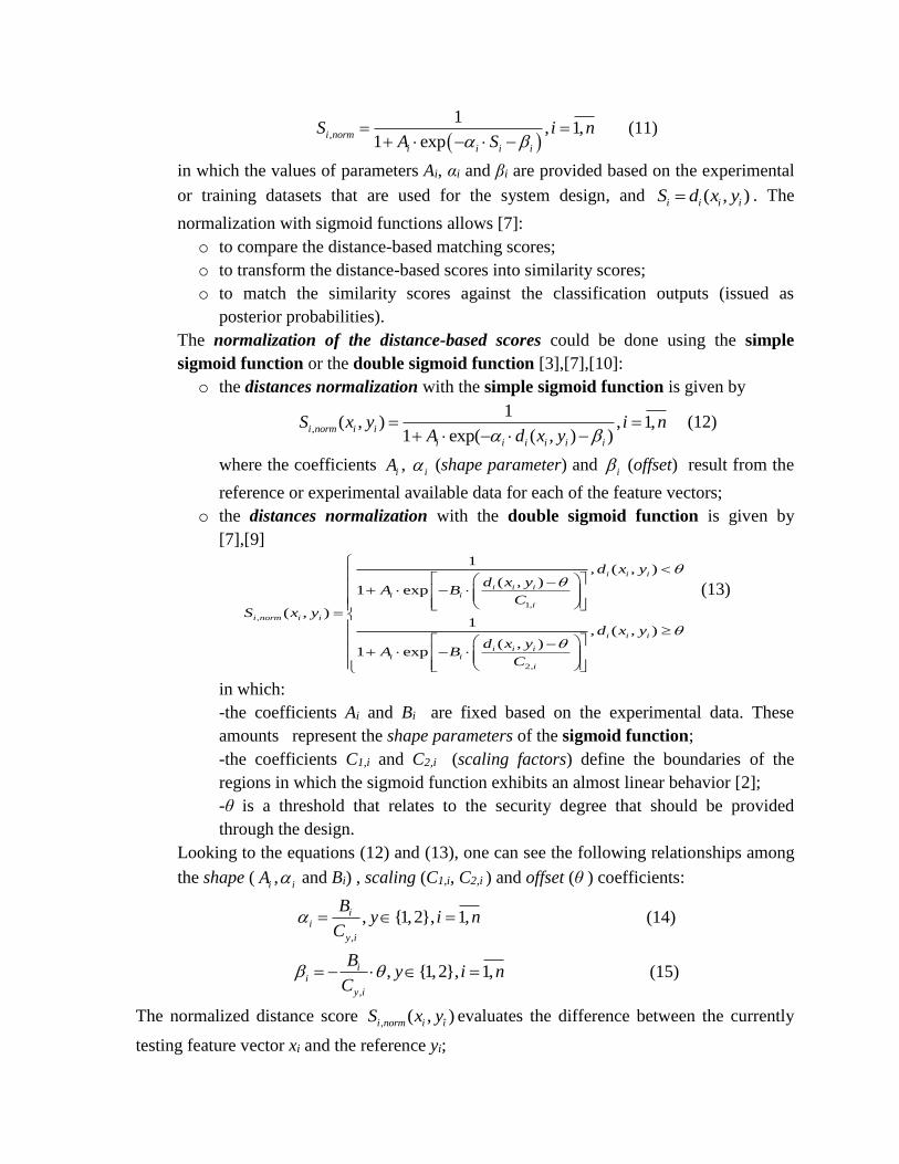
the learning curves representation to find out the optimal learning models with the
properly fixed training samples per class. The learning curve for a classifier is a graphic
representation of some performance measures (typically the average classification error
rate for all the considered classes) in respect to the available training set size (the number of
training samples per class). The learning curve allows to properly fix the training dataset
size and also to compare several classification models for various sizes of the available
training dataset. An example of learning curve representation for several models that run on
a difficult dataset for a fingerprint recognition system is given in figure 1. A difficult dataset
is one in which the separation within the classes if difficult, sometimes because of an intra-
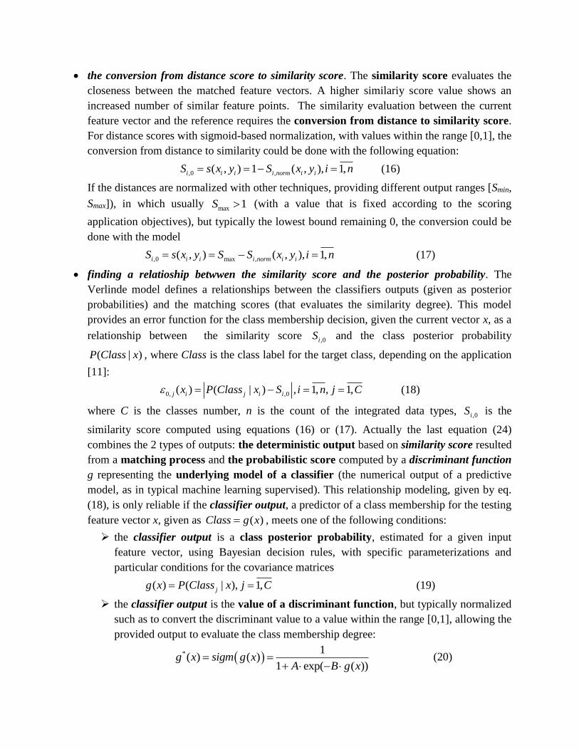
class variance that significantly excedd the overall inter-class variance. The learning curve
for a classifier shows that an ideal model has a performance that asymptotically is going to
the minimum classification error rate (Bayes error [2],[5],[12]), as depicted in figure 2.
Figure 1: Learning curves for several classifiers on difficult dataset
Figure 2: Learning curves for the optimal (ideal) classifier: the asymptotic
generalization and apparent error rates [1],[12]
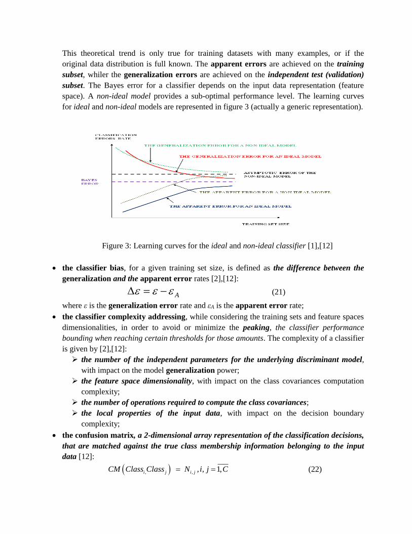
This theoretical trend is only true for training datasets with many examples, or if the
original data distribution is full known. The apparent errors are achieved on the training
subset, whiler the generalization errors are achieved on the independent test (validation)
subset. The Bayes error for a classifier depends on the input data representation (feature
space). A non-ideal model provides a sub-optimal performance level. The learning curves
for ideal and non-ideal models are represented in figure 3 (actually a generic representation).
the classifier bias, for a given training set size, is defined as the difference between the
generalization and the apparent error rates [2],[12]:
A (21)
where ε is the generalization error rate and εA is the apparent error rate;
the classifier complexity addressing, while considering the training sets and feature spaces
dimensionalities, in order to avoid or minimize the peaking, the classifier performance
bounding when reaching certain thresholds for those amounts. The complexity of a classifier
is given by [2],[12]:
the number of the independent parameters for the underlying discriminant model,
with impact on the model generalization power;
the feature space dimensionality, with impact on the class covariances computation
complexity;
the number of operations required to compute the class covariances;
the local properties of the input data, with impact on the decision boundary
complexity;
the confusion matrix, a 2-dimensional array representation of the classification decisions,
that are matched against the true class membership information belonging to the input
data [12]:
, , , , 1, i j i jCM Class Class N i j C (22)
Figure 3: Learning curves for the ideal and non-ideal classifier [1],[12]

where , i jN is the number of the examples belonging to the true class Ci while the classifier
decision is for the class Cj. The confusion matrix rows contain the true class labels for the
input samples (as row indices); the columns index the classifier output decisions on the input
data. The confusion matrix entries count the matching between the true class labels and the
classifiers decisions, for each of the specified classes. The diagonal entries store the right
classifiers decisions while the non-diagonal entries store the wrong decisions about class
membership;
the usage of cross-validation techniques in order to enhance the generalization power of
the designed model, such as to prevent or reduce the over-fitting of training data [4]. The
cross-validation is a classifier design and evaluation technique that looks to improve its
generalization performance by running several rounds of training and validation, with
varying the used datasets. Within each round, the design dataset is partitioned into
complementary subsets; the classifier training is done on one subset, and the validation is
performed on the remaining subset or examples that were not used for training. Several
rounds are run with different partitioning of the design dataset [12];
the classes unbalancing approaching as concerning the number of training samplers per
class and the classes representation within the training dataset;
the classifier selection methodology, with the following steps [4],[12]:
1. providing the relevant datasets for the security system design and testing;
2. starting the design (training/learning) process with the lowest complexity models
(e.g. NMC, Fisher and LDC). These models provides good performances when the
training dataset contains a small number of samples per class;
3. testing the models in their increasing complexity order;
4. comparing the performances on training and testing (validation) datasets, using the
learning curves.
The selection and evaluation of an optimal model for the application goals (the desired security
performance) require to take in account the peaking. This means that the generalization power of
the model is constrained by the ratio between the Training set Size (TS)-the number of training
samples per class- and the problem complexity given by the Feature set Size (FS)-the number of
used features. A required condition for a good generalization performance is the following
[2],[6]: maximization of the ratio TS
FS, TS FS .The peaking is depicted in figure 4 [1],[2]. The
peaking means that for a given training set size (TS) and with a significant increasing of the
feature space size (FS), the classification errors rate reduction is only achieved till reaching a
certain boundary that constrains the overall performance of the designed system. Therefore, if
the provided features number FS exceeds a certain threshold FS0, the performance trend reverses
and it does not more happen what it was normally expected for an extended feature set; therefore
in this case the classification errors rate actually starts to increase. From figure 4 one can see that
the critical threshold of the features number (parameter FS) moves to the right of the

horizontal axis, therefore towards the higher values with the increasing of the training samples
number. A minimum value for this threshold is reachable according to [2]
* TSFS
(23)
where the coefficient α must meet the bounding condition [2,10] , that is typically for the best
performances.
2.2 The learning (modeling) process optimization
The learning or modeling process could be significantly improved to provide high performance
according to the real security application if some design options are applied. These functional
options include the following technical approaches:
Moving from multi-class to binary classification;
Applying a target-vs.-non-target classification, typically within a hierarchical classifier in
order to design multi-level security systems.
a) Transition from multi-class to binary classification
The typical methods that could be applied in order to build multi-class models using several
binary classification models are the following [4],[13],[14]:
One-vs.-all others method;
One-vs.-one method;
DDAG (Decision Directed Acyclic Graph)-based method.
b) Target vs. non-target classification and hierarchical classification
It is a design approach that is suitable for multi-level security applications in which the end-users
have various roles and authorization degrees. The design is based on 2 classification techniques:
Detector classifiers, that are trained to separate between a target and a non-target class;
Discriminant classifiers, in which the training process is done for all classes.
Figure 4: The performances peaking, for some given values of the Training set Size (TS) and
Feature set Size [1],[2]
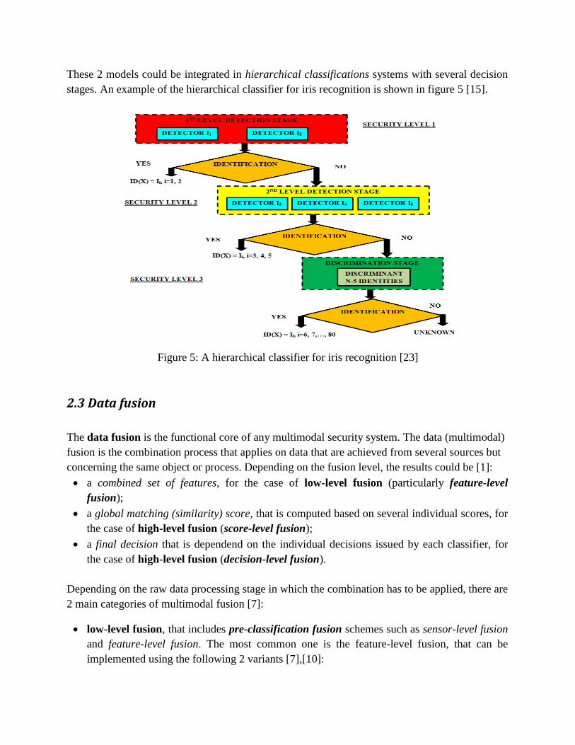
These 2 models could be integrated in hierarchical classifications systems with several decision
stages. An example of the hierarchical classifier for iris recognition is shown in figure 5 [15].
2.3 Data fusion
The data fusion is the functional core of any multimodal security system. The data (multimodal)
fusion is the combination process that applies on data that are achieved from several sources but
concerning the same object or process. Depending on the fusion level, the results could be [1]:
a combined set of features, for the case of low-level fusion (particularly feature-level
fusion);
a global matching (similarity) score, that is computed based on several individual scores, for
the case of high-level fusion (score-level fusion);
a final decision that is dependend on the individual decisions issued by each classifier, for
the case of high-level fusion (decision-level fusion).
Depending on the raw data processing stage in which the combination has to be applied, there are
2 main categories of multimodal fusion [7]:
low-level fusion, that includes pre-classification fusion schemes such as sensor-level fusion
and feature-level fusion. The most common one is the feature-level fusion, that can be
implemented using the following 2 variants [7],[10]:
Figure 5: A hierarchical classifier for iris recognition [23]
concatenation-based fusion, typical for heterogeneous feature vectors (with different
sizes);
functional combination fusion, that could be applied for feature vectors with the same
sizes.
high-level fusion, that includes post-classification fusion schemes such as score-level
fusion, rank-level fusion and decision-level fusion. The score-level fusion is the most
implemented one, typically based on several mathematical rules for scores combination (for
example sum rule, average rule, min-rule). Some of these fusion rules could be provided
with parameters such as various weigths.
3. Performance measures for the security systems based on
multimodal technologies
The overall design and development process of security systems using multimodal technologies
requires a carefull consideration of the performance issues, in order to meet the real application
constraints.
Under this methodological framework, and taking in account the typical functional components
of any multimodal security system, a classifier performance is evaluated using the following
approaches [16]:
the training performance, that evaluates the classifier capability to make right decisions on
the class membership for the training samples (therefore the training optimization);
the generalization performance, that evaluates the classifier capability to identify the class
membership for the new (unseen) examples.
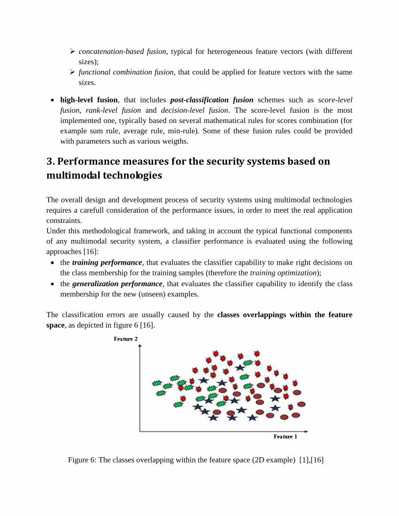
The classification errors are usually caused by the classes overlappings within the feature
space, as depicted in figure 6 [16].
Figure 6: The classes overlapping within the feature space (2D example) [1],[16]
The typical reasons of the classes overlapping within the feature space are the following
[1],[2],[5],[16]:
a poor feature space dimensionality, that is not enough to cover the overall set of attributes;
the low relevance of the extracted features, that do not describe the most useful discriminant
properties;
the noise and outliers within the input datasets.
The security performances of the multimodal systems are evaluated using amounts that relate to
the positive (P)/negative (N) outputs of the predictive model. The following amounts are
typically used to define the security performances [1],[12]:
TP (True Positive): the count of right decisions for a target class (the positive class for the
application). A true positive decision is generated when the predicted value P is the same as
the real (true) value;
TN (True Negative): the count of right decisions for a non-target class (the negative class).
A true negative decision is generated when both values (predicted and real) are N;
FP (False Positive, Type I Error): the count of wrong decisions for the target (positive)
class. A false positive decision (false alarm/alert) is generated when the predicted value is
P but the real value is N;
FN (False Negative, Type II Error): the count of wrong decisions for the non-target
(negative) class. A false negative decision is generated when the predictor output is N but
the real value is P.
The following security performances are computed based on the above amounts [1],[12]:
TPR (True Positive Rate, sensitivity, detection rate/probability), given by
TPTPR
TP FN
(24)
TNR (True Negative Rate, specificity), given by
TNTNR
FP TN
(25)
FPR (False Positive Rate, fals alarms/alerts rate/probability), given by
1#
FP FPFPR TNR
N FP TN
(26)
where #N is the total amount of decisions for the non-target class;
FNR (False Negative Rate), given by
1#
FN FNFNR TPR
P FN TP
(27)
where #P is the total amount of decisions for the target class
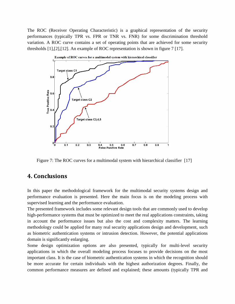
The ROC (Receiver Operating Characteristic) is a graphical representation of the security
performances (typically TPR vs. FPR or TNR vs. FNR) for some discrimination threshold
variation. A ROC curve contains a set of operating points that are achieved for some security
thresholds [1],[2],[12]. An example of ROC representation is shown in figure 7 [17].
4. Conclusions
In this paper the methodological framework for the multimodal security systems design and
performance evaluation is presented. Here the main focus is on the modeling process with
supervised learning and the performance evaluation.
The presented framework includes some relevant design tools that are commonly used to develop
high-performance systems that must be optimized to meet the real applications constraints, taking
in account the performance issues but also the cost and complexity matters. The learning
methodology could be applied for many real security applications design and development, such
as biometric authentication systems or intrusion detection. However, the potential applications
domain is significantly enlarging.
Some design optimization options are also presented, typically for multi-level security
applications in which the overall modeling process focuses to provide decisions on the most
important class. It is the case of biometric authentication systems in which the recognition should
be more accurate for certain individuals with the highest authorization degrees. Finally, the
common performance measures are defined and explained; these amounts (typically TPR and
Figure 7: The ROC curves for a multimodal system with hierarchical classifier [17]
FPR) are used to optimize the designed system accuray according to the customer application
requirements. The application key target indicators (detection rate vs. alert rate) are based just on
these amounts (TPR and FPR , respectivelly). The real application goal is to maximize the
detection rate (TPR) for a certain alert rate (FPR) that should be as low as possible.
References
[1] Sorin Soviany, Sorin Puşcoci: Soluţii multimodale pentru securizarea serviciilor
mobile, Editura AGIR, 2016
[2] Sergios Theodoridis, Konstantinos Koutroumbas: Pattern Recognition 4th edition,
Academic Press, Elsevier, 2009 ISBN 978-1-59749-272-0
[3] David Zhang, Fengxi Song, Yong Xu, Zhizhen Liang: Advanced Pattern Recognition
Technologies with Applications to Biometrics, Medical Information Science Reference,
IGI Global, 2009
[4] ***: Curs Pattern Recognition: Classification, Discriminant Analysis, Universitatea
Delft, Olanda, 2009-2010
[5] Luc Devroye, Laszlo Gyorfy, Gabor Lugosi: A Probabilistic Theory of Pattern
Recognition, Springer, 1997, ISBN 0-387-94618-7
[6] Andrew R. Webb, Keith D. Copsey: Statistical Pattern Recognition, 3rd edition,
Wiley, 2011
[7] A. Jain A., K. Nandakumar K., A. Ross: Score Normalization in multimodal biometric
systems, Pattern Recognition, The Journal of the Pattern Recognition Society, 38
(2005)
[8] Supriya Kapoor, Shruti Khanna, Rahul Bhatia: Facial Gesture Recognition using
Correlation and Mahalanobis Distance, (IJCSIS) International Journal of Computer
Science and Information Security, Vol. 7, Nr.. 2, 2010
https://arxiv.org/ftp/arxiv/papers/1003/1003.1819.pdf
[9] Arun Ross, Anil K.Jain: Multi-Modal Biometrics: An Overview, 12th European Signal
Processing Conference (EUSIPCO), Viena, Austria, septembrie 2004 ,
http://www.csee.wvu.edu/~ross/pubs/RossMultimodalOverview_EUSIPCO04.pdf
[10] R.Snelick, M.Indovina: Multimodal biometrics: issues in design and testing,
Proceedings of 5th International Conference on Multimodal Interfaces, Canada, 2003,
pp. 68-72 http://visgraph.cs.ust.hk/biometrics/Papers/Multi_Modal/ICMI_11_2003.pdf
[11] P.Verlinde, P.Druyts, G.Cholet: Applying Bayes classifiers for decision fusion in a
multi-modal identity verification system, Proceedings of International Symposium on
Pattern Recognition, Belgium, 1999
[12] *** : PerClass Training Course: Machine Learning for R&D Specialists, Delft,
Netherlands
[13] Kai-Bo Duan, S. Sathiya Keerthi: Which Is the Best Multiclass SVM Method? An

Empirical Study, Springer-Verlag Berlin Heidelberg 2005
http://www.keerthis.com/multiclass_mcs_kaibo_05.pdf
[14] John C. Platt, Nello Cristianini, John Shawe-Taylor : Large Margin DAGs for
Multiclass Classification, S.A. Solla, T.K. Leen and K.-R. M¨uller (eds.), 547–553,
MIT Press (2000)
http://citeseerx.ist.psu.edu/viewdoc/download?doi=10.1.1.99.5506&rep=rep1&type=p
df
[15] Sorin Soviany, Cristina Soviany, Sorin Puşcoci: An Optimized Iris Recognition System
for Multi-level Security Applications, The 2014 International Conference on Security
and Management (SAM'14), World Academy of Science, Las Vegas, SUA, July 21-24,
2014
[16] Robi Polikar: Pattern recognition, Wiley Encyclopedia of BioMedical Engineering,
2006 http://users.rowan.edu/~polikar/RESEARCH/PUBLICATIONS/wiley06.pdf
[17] Sorin Soviany, Virginia Săndulescu, Sorin Puşcoci: The Hierarchical Classification
Model using Support Vector Machine with Multiple Kernels in Human Behavioral
Pattern Recognition, The 6th IEEE International Conference on E-Health and
Bioengineering - EHB 2017 Grigore T. Popa University of Medicine and Pharmacy,
Sinaia, România, June 22-24, 2017
Top Related