HYBRID GENETIC ALGORITHM FOR ASSEMBLY LINE BALANCING … Brudaru(ac. 2).pdf · HYBRID GENETIC...

BULETINUL INSTITUTULUI POLITEHNIC DIN IAŞI Publicat de

Universitatea Tehnică „Gheorghe Asachi” din Iaşi Tomul LIV (LVIII), Fasc. 2, 2008

Secţia AUTOMATICĂ şi CALCULATOARE

HYBRID GENETIC ALGORITHM FOR ASSEMBLY LINE BALANCING WITH FUZZY TIMES AND PARALLEL

WORKSTATIONS

BY

OCTAV BRUDARU, BRENT VALMAR and *D. POPOVICI

Abstract. This paper deals with the design of balanced assembly lines with parallel

workstations in the case when the execution times are real sampled fuzzy numbers. The need for parallel workstations appears whenever the assembly process contains some tasks whose processing times are longer than the cycle time. The variant when the execution times are fuzzy number was considered as a better compromise between the reality modelling and the efficiency of the solving techniques. In order to solve this problem, it is proposed an efficient greedy algorithm that constructs an assembly structure containing both serial and parallel workstations for a prescribed confidence threshold. An optimal detecting criterion allows the obtaining of a simple relationship between the solution given by the algorithm and an easily calculated lower bound of the number of serial and parallel workstations. The greedy algorithm is grafted on a genetic algorithm resulting a powerful tool for solving this problem The performance of the hybrid genetic algorithm related to efficiency of defuzzyfication rules, optimality of the number of workstations, absolute and relative deviation from the optimal value, are experimentally analyzed.

Key words: assembly line balancing, parallel workstations, fuzzy numbers, hybrid genetic algorithm, greedy method.

2000 Mathematics Subject Classification: 68R10, 68T27.

1. Introduction

The paradigm of assembly line balancing appeared in the industrial domain of the Ford Systems 80 years ago. Since its first mathematical formulation [22] this problem was both intensively and extensively studied in order to find more efficient solving methods and to extend the model for

52 Octav Brudaru, Brent Valmar and D. Popovici

handling new constraints. The study of this problem remains of a continuous interest [23].

Assembling is one of the most important stages in manufacturing. The product is basically composed by many components. In some sense, assembling the product is to materialize by mechanic means the logical links existing among the different parts [5]. An assembly process is the logical, then chronological specification of a set of given functions that transform the components into a product. The realization of the process is based on different timings or chronologies that range from pure sequential to partial parallel. The realization of each function involves the execution of a specific task and each task requires a processing time. Further, we consider only serial chronologies of the assembly process when the corresponding physical structure is an assembly line. Usually, it is assumed that the execution time of each task is a positive real number.

Basically [5], the assembly line balancing (ALB) problem consists in the grouping of a set V of tasks into workstations so that the precedence constraints in the execution of tasks are respected ([2], [3], [4]). The precedence constraints are given by an acyclic directed graph ),( AVG = in which V is the set of tasks and the set of arcs and expresses the precedence between tasks. In the deterministic case, the execution time of each task is a positive real number. The products (batches) move along the assembly flow which passes through a number of workstations. The tasks within each workstation are serially executed. The execution time of tasks belonging to a workstation does not exceed a positive real number C , called cycle time. The batch moves from current workstation to the next one at every C units of time. Idle time appears whenever the processing times of workstations are less that the cycle time. The first product leaves the line after units of time, whilst the remaining ones with the rate of one at every C units of times. The objective is to group the tasks into workstations so that the total idle time is minimized and this is equivalent to the minimization of the number of workstations when the cycle time is constant [23].

A

mC

It is worth mentioning that this problem appears in any type of industry that involves assembly processes. Whilst the ALB problem is HP-hard, the heuristic methods are the unique efficient solving tool, even if these techniques do not guarantee the optimality of sought solution. The deterministic case of ALB was extensively investigated with respect to mathematical models and solving techniques [22], [16], [26], [23].

Recently - maybe due the appearing of genetic algorithms as a versatile tool – the variant when the execution times are fuzzy number was considered as a better compromise between the reality modelling and the efficiency of the solving techniques [27], [6], 7]. The natural question concerning this aspect is: Why a fuzzy approach? The behaviour of the real world systems has a certain degree of uncertainty and the input data - in present case the execution times -

Bul. Inst. Polit. Iaşi, t. LIV (LVIII), f. 2, 2008 53

can only be estimated. Also, the working of the assembly line in real conditions has uncertain aspects. The nondeterministic case is essentially related to the nondeterministic behaviour of task execution times. So, the stochastic case considers these times are random variables with a know distribution [21], [25]. The first approach in handling these aspects was to consider that the execution times are random variables [25]. In this context, the condition to be satisfied by a solution is reformulated while the objective is to minimize the mean of the total idle time under the assumption that the processing times are random variables. Although this stochastic model approximates better the reality, the higher complexity of the solving techniques comes as price. So, it should be realized a compromise between the accuracy of the model and the complexity of the algorithms to solve it. The best solution is to consider that the execution times are sampled real fuzzy numbers [17]. This is because a fuzzy number can reflect the vague feature of the both predicted and realized processing times while the mathematical tools are simple [6], [9].

In this paper it is considered the design of balanced assembly lines with parallel workstations in the case when the execution times are real sampled fuzzy numbers [17]. The need for parallel workstations appears whenever the assembly process contains some tasks whose processing times are longer than the cycle time. In [12] some design criteria and heuristics can be found. On the other hand, the nondeterministic case is essentially related to the behaviour of task execution times. The variant when the execution times are fuzzy number was considered as a better compromise between the reality modelling and the efficiency of the solving techniques. In order to solve this variant of the problem, it is proposed an efficient greedy algorithm that constructs an assembly structure containing both serial and parallel workstations for a prescribed confidence threshold. The algorithm is based on certain optimization measures induced by different defuzzyfication rules. An optimal detecting criterion allows the obtaining of a simple relationship between the solution given by the algorithm and an easily calculated lower bound of the number of serial and parallel workstations. The performance of the hybrid genetic algorithm related to efficiency of defuzzyfication rules, optimality of the number of workstations, absolute and relative deviation from the optimal value, are experimentally analyzed.

The rest of the paper is organized as follows. In section 2, the mathematical model for ALB with fuzzy overtime tasks is described. The optimality condition is defined for the case of parallel workstations in section 3. A greedy algorithm that combines the greedy approach from the previous section with the approximation method for the deterministic case described in [BruM00] is described in section 4. In section 5 it is proposed a hybrid genetic algorithm combining the greedy method for parallel workstation with a slightly different version of the genetic algorithm for serial workstations. The results of some numerical investigations are given in Section 6. Last section summarizes the work.


2. Mathematical Model for ALB with Fuzzy Overtimes It is recalled that the assembly line balancing model uses an acyclic

digraph , where G=(V,A) n}{1,2,...,=V is the set of tasks and is the set of arcs. Task precedes task

VVA ×⊂i j if and only if Aji ∈),( . If Aji ∈),(

i

then the execution of can begin only if task is completed. Let t be the execution fuzzy time of task , . It is denoted the value of the desired cycle time of the assembly line. For each task , consider the sequence of pairs

j

(),...,, 11 ii

in,...,1

))ik

i

ik

i =

,

Ci

((it μθμθ= , where 0>ijθ is a realization of the execution time and ijμ represents the value of the membership function for ijθ ,

]1,0[∈ijμ , ,k,j …=1 . The basic operations for the handling of the fuzzy times like addition of two fuzzy numbers, comparing a fuzzy number with a real one and defuzzyfication are described below.

2.1. Fuzzy Arithmetic

In this section the fuzzy approach model of the assembly line balancing

problem is presented. The formulating of the ALB problem with fuzzy times requires some basic elements of the fuzzy arithmetic. Next, they are reviewed the fuzzy addition of real sampled fuzzy numbers, a way to compare a fuzzy number with a real number and some defuzzyfication rules.

2.1.1. Addition of two sampled fuzzy numbers. The arithmetic of the –

sampled real fuzzy numbers is defined in [17]. Consider two sampled real fuzzy numbers

k

)),(),...,,(( 11 kk pxpxx = and )),(),...,,(( 11 kk qyqyy = , where and , are the value of membership functions for and and

, Ryx ii ∈,

iyip iq ix

[ ] ki ,...,1,1,0 =∈qp ii , . If yxz += and ( ) ( )( )kk rzrzz ,,...,, 11=

z then the following steps are to

be executed for computing [17]: 1. Compute 110 yxa += , nnn yxa += , ( ) kaah n /0−= , ,

. haa ii += −1

1,...,1 −= ni2. Take , [ ]101 , aaI = ( ]iii aaI ,1−= , ki ,...,2= ; 3. Compute jiij yxs += , ( ) kjiqp jiij ,...,1,,,min ==μ

4. For each execute: kh ,...,1=a) compute }/{ hjiijh IssS ∈= , kh ,...,1= ;

b) if then take ∅≠hS ** jih sz = and **, jihr μ= , where and

hji Ss ∈**

{ }hijji Ss ∈=** ij /max μμ , else take 2/)1 hh aa(hz += − and . 0=hr


Note that ( ) ( )( 1,0,...,1,0=u )verifies that xxuux =+=+ for any sampled real fuzzy number x .

2.1.2. Comparison of two fuzzy numbers. First, it is necessary to

compare a fuzzy number with a real number α in order to formulate that fact that the processing time of each workstation does not exceed the cycle time. The most appropriate way in this context is to compute:

( ) [ ]1,0

1

∈=≤

∑

∑

=

≤k

ii

xi

p

pxConf i αα

and to compare it with a given threshold value ( ]1,00 ∈c , namely

( ) 0cxconfxdef

≥≤⇔≤ αα

The value of ( )α≤xConfx′

can be regarded as a measure of confidence of the fact that -values are less than α [Kao76]. Observe that

nixi ,...,1, => α implies that ( ) 0=≤ αxConf , whilst α≤ix for leads to

ni ,...,1=( ≤ ) 1=αxConf . The above threshold ensures the desired degree of

constraint satisfaction. A full satisfaction corresponds to 10 =c , whilst no satisfaction is for c . 0=0

2.1.3. Defuzzyfication rules. The greedy algorithm described in section

2.2 constructs each workstation by assigning one task at a time. This task is extracted from a list of assignable tasks according to some selection criteria. Such a criterion should indicate as favourite those tasks that fill better the existing idle time in the current workstation, and this requires the ranking of the tasks. This is done using a defuzzyficator that associates a real number to a fuzzy number. This real number is viewed as the most a representative value of that fuzzy number. In this order we consider five defuzzyfication formulas for ranking the tasks [15]. In each case )),(),...,,(( 11 kk pxpxx = denotes the fuzzy number whose defuzzyfied value is computed.

a) the maximum

( ) jj

ii ppxxd max, **1 ==

b) the mean of maximum


( ) jj

ii

l

jij pppx

lxd

lmax...,1

11

2 ==== ∑=

c) the centre of gravity method

( )∑

∑

=

==k

ii

k

iii

p

pxxd

1

13

d) the weighted maximum

( ) jj

iii pppxxd max, ***4 ==

e) the confidence of fitness

( ) ( )CxtConfCtxd ≤+−=1,,5

2.2. Mathematical Model

Let be a partition of V so that },{ 21 VV })(,/{ 01 cCtConfViiV i ≥≤∈=

and })2 0cCti ≥( )({ 02 ConfcCtConfV i and,/ Vii ≤<≤=

1V)

∈

(WTW

. Each is called an overtime task, while each task in is called a normal task. If let us denote by the sum of the processing fuzzy time of tasks belonging to . Let be the set of all partitions, W

2Vi∈VW ⊂

},...,{ 1 mWWW = of , that satisfy the following conditions:

V

(1) if Ayx ∈),( , rWx∈ and sWy∈ then sr ≤ ,

(2) 0))((( cCWTConf j ≥≤ , if ∅=∩ 2VW j ,

(3) 0)2)((( cCWTConf j ≥≤ if ∅≠∩ 2VW j .

Each member of is a solution to the problem and are the corresponding workstations. A solution with a minimum

number of workstation is an optimal one. Further, we shall suppose that is acyclic and for each

},...,{ 1 mWWW =

0)2) cCW j ≥≤

W

mWW ,...,1G

(((TConf Vi∈ and this guaranties that the solution set W is nonempty. The problem is to find an optimal solution. The above stated optimization problem is NP-hard while its corresponding decision


problem is NP – complete. Consider a solution },...,{ 1 nWWW = and suppose that contains an overtime task. Since jW 0)2)( cCWT j ≥(Conf ≤ it results that we can create a cell by putting a copy of that acts in parallel with the original. The period of the resulted cell is time units even if its response time is . Station is called parallel station. No need for a parallel copy appears when does not contain an overtime task (such a station is called serial).

jWC

C

jW2 jW

sm +Therefore, the assembly line works with a number of virtual serial

stations pv m2m = , where ( ) represents the number of serial (parallel) workstations in the solution. Clearly,

sm pm

ps mmm += . The number is used for detecting the optimality of the corresponding solution. m s

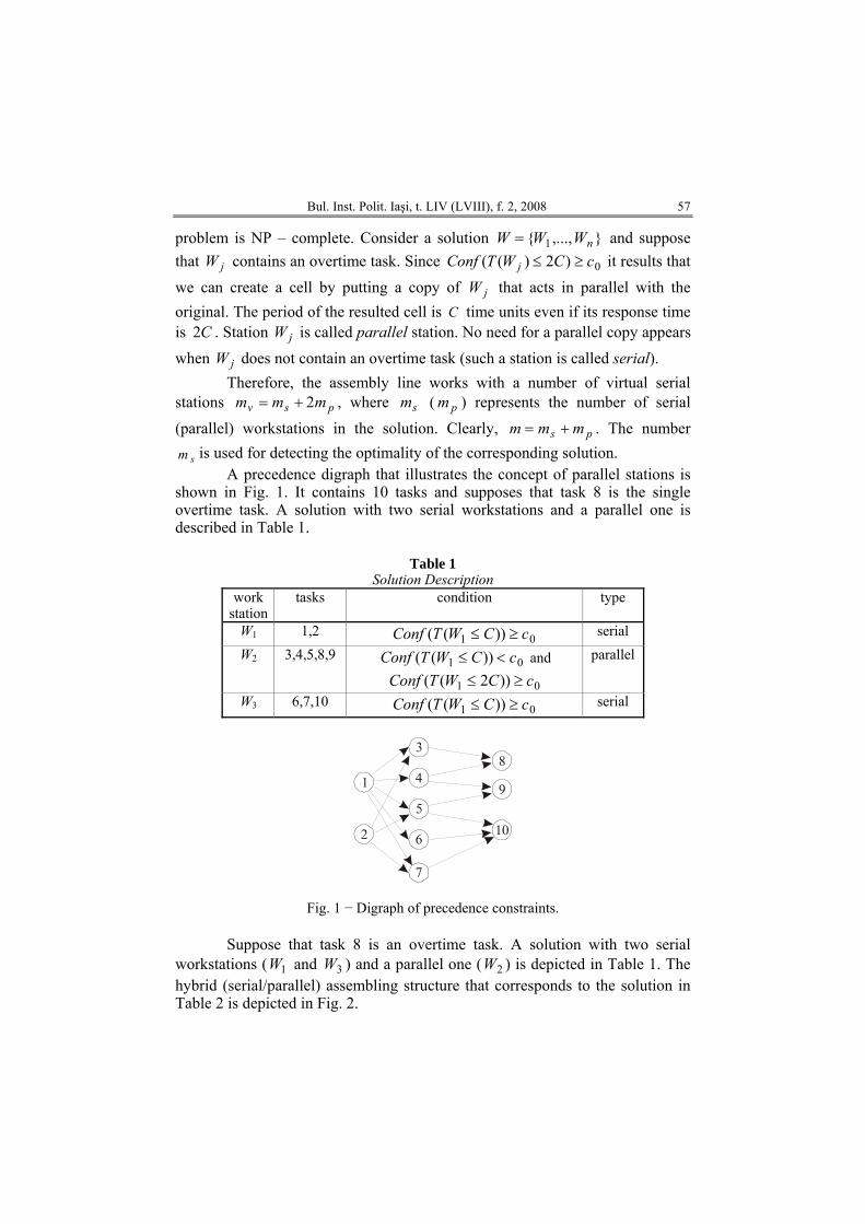
A precedence digraph that illustrates the concept of parallel stations is shown in Fig. 1. It contains 10 tasks and supposes that task 8 is the single overtime task. A solution with two serial workstations and a parallel one is described in Table 1.

Table 1 Solution Description

work station

tasks condition type

W1 1,2 0))( cTConf ≥1 C(W ≤ serial W2 3,4,5,8,9 0(( cTConf 1W ))C≤ < and

0))( cTConf ≥1(W 2C≤

parallel

W3 6,7,10 0))( cTConf ≥ serial 1 C(W ≤

1

2

5

4

3

9

8

6

7

10

Fig. 1 − Digraph of precedence constraints.

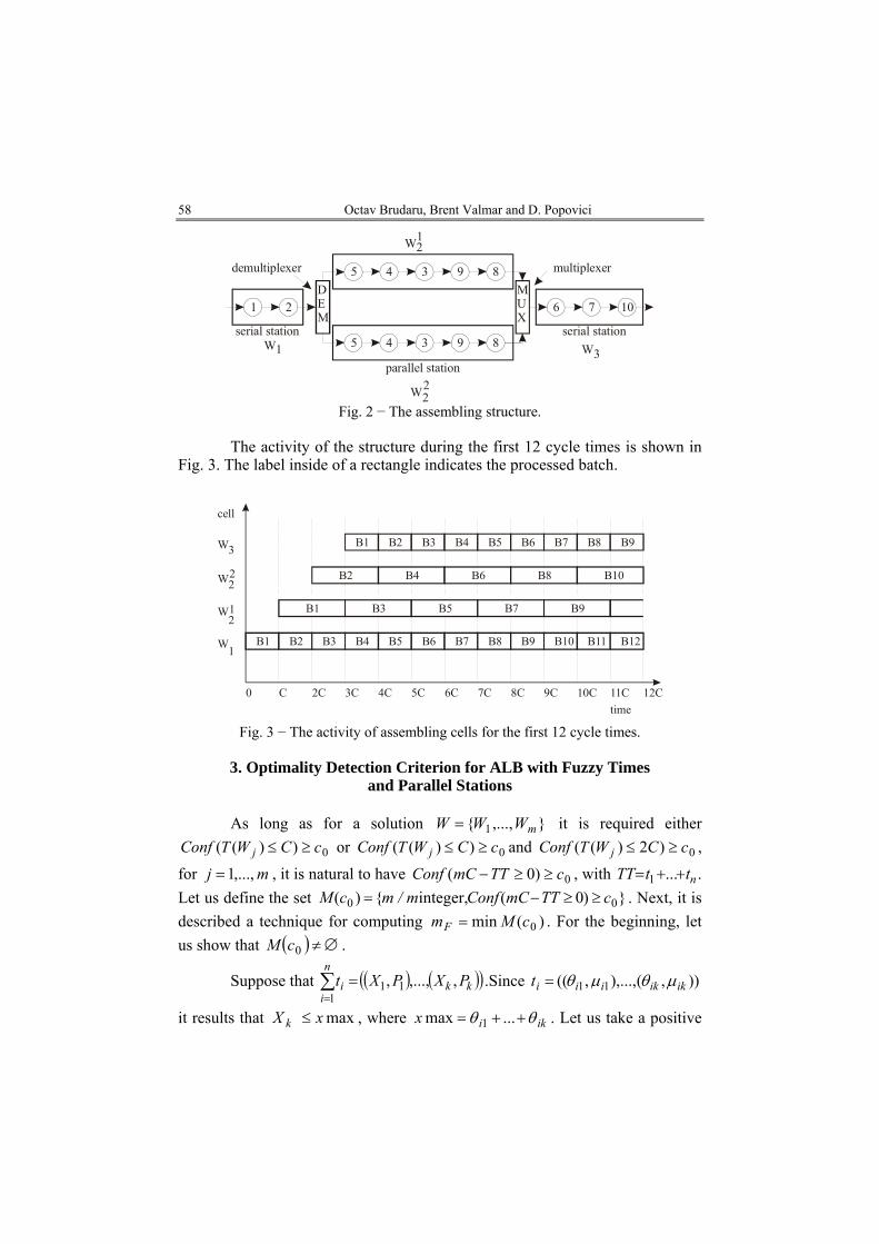
Suppose that task 8 is an overtime task. A solution with two serial workstations ( and ) and a parallel one ( ) is depicted in Table 1. The hybrid (serial/parallel) assembling structure that corresponds to the solution in Table 2 is depicted in Fig. 2.

1W 3W 2W


1 2

5

5

4

4

3

3

9

9

8

8

6 7 10DEM

MUX

demultiplexer

parallel station

serial stationserial station

multiplexer

W1

W12

W22

W3

Fig. 2 − The assembling structure.

The activity of the structure during the first 12 cycle times is shown in

Fig. 3. The label inside of a rectangle indicates the processed batch.

C0 2C 3C 4C 5C 6C 7C 8C 9C 10C 11C 12

W1

W21

W22

W3

time

cell

B1

B1

B2

B2

B3

B3

B4

B4

B5

B5

B6

B6

B7

B7

B8

B8

B9

B9

B10 B11 B12

B2

B3

B4

B5

B6 B8 B10

B7 B9B1

C

Fig. 3 − The activity of assembling cells for the first 12 cycle times.

3. Optimality Detection Criterion for ALB with Fuzzy Times and Parallel Stations

As long as for a solution },...,{ 1 mWWW = it is required either

0))(( cCWTConf j ≥≤ or 0)) cCj ≥(( WTConf ≤ and ,

for , it is natural to have Conf0)2)(( cCWTConf j ≥≤

0cmj ,...,1= )0( TTmC ≥≥− , with . Let us define the set

nttTT ++= ...1

})0 0c≥≥(integer, TTmCConf {) m / m( 0cM −= . Next, it is described a technique for computing )(min 0cMmF = . For the beginning, let us show that . ( ) ∅≠0cM

Suppose that .Since ( ) (( )kk

n

ii PXPXt ,,...,, 11

1=∑

=) )),(),...,,(( 11 ikikiiit μθμθ=

it results that , where maxx ix X k ≤ ikθθ ++= ...max 1 . Let us take a positive


integer such that . It is obtained thatm Cxm max/≥ khCmX h ,...,1, =⋅≤ . From the definition of the confidence (1) and the fact that

k X XX <…<<1

)/( ≤ CmConfi

we obtain that and therefore

.

∑=

=k

hki P

1∑≤ mCx

Pi

2

1∑=

tn

i 1=

( )0c , i.e. ( )Mm∈ ∅This implies that ≠0cM

(mC

. On the other hand, for

any , we obtain that because

, implies that

0

1=

≤m

h,0

0)01

=≥− ∑=

n

iit

khX h ,...,1,0

Conf

x ih ,...,≥ nik ,...,1, = =≥ , i.e. . This implies that k,...,h,0X h ≤mC 1=− ( )0cM has a non-negative lower

bound. Actually, it was proved that ( )0cmin MmF = is well defined and we obtained the optimality test in the fuzzy case: if { } 1 m, W, WW …= is a solution to the fuzzy ALB problem then Fmm = implies that W is an optimal solution.

Now, let us show that the function [ ]1,0:f →N

⎜⎜⎝

⎛−≤−=⎟⎟

⎠

⎞∑=

tmCConfn

ii

1

0≥

where

is an increasing function. ( ) (f −= mCm 0)1

≥∑=

n

iit

( ) ⎜⎜⎝

⎛=+ Confm (1

),f(m=

Conf

mC −

Indeed,

because for any so that

≥⎟⎟⎠

⎞≥−+ ∑

=CtCm

n

ii

10)1f

0⎟⎟⎠

⎞ h1tConf

n

ii⎜⎜

⎝

⎛≥∑

=

− hXmC it results

i.e. CmC −− X h ≥ ∑∑∑≥− ≥−

. 0hXmChP

+−≥−=≤

0hXChP

)1(h mCXmChP

Let us take ( )Cmax/xceilmRIGHT mLEFT and 0=( )

= . As in the previous section, we have ( )f and 10f ==LEFTm

fRIGHTm

Fm. The algorithm below

exploits the monotony of and finds using the binary search. Algorithm for calculating the lower bound Fm1. ( )CxmLEFT max/ceilmRIGHT ;0 == ;

2. do { ( ) 2/ RIGHTmm LEFTMIDLE m ; +=

( ) 0MIDLE Cm RIGHT m m = if f ;MIDLE≥

m

else MIDLELEFT m= ;

} until ( );1 +=RIGHT mm MIDLE


3. ; RIGHTF mm =

In the case of serial workstations it is proved that for each solution with workstations, it followsm mmF ≤ . Therefore, whenever mmF = holds for a

solution with m workstations then this solution is optimal. The above test assumes that fuzzy time of each workstation is up to C .

On the other hand, in the case of parallel stations, a solution with workstations could have serial stations and double parallel ones, where

msm pm

ps mmm += . So, instead of comparing with we have to compare with the number of virtual serial workstations

Fm mmFm psv mm ⋅+= 2 . If

holds for a certain solution than we conclude that it is an optimal one. This criterion is used in experimental investigation for measuring the algorithm performance by counting the cases when an optimal solution is detected. Since this criterion acts as a sufficient condition, actually the real performance could be better because a solution can be optimal even if the test above cannot detect its optimality.

vmFm =

Now, consider the example in the previous section. For and it results , and for

10=C75.00 =c 3=Fm 2.5=C and 8.00 =c it is obtained . Since the number of virtual serial workstations we obtained is

and, respectively, it is concluded that both solutions are optimal. 6=Fm=vm

3=vm6

4. A Greedy Algorithm

In this section, it is presented a greedy algorithm for solving the ALB

problem, with fuzzy overtime tasks and it is applied to an example. The option for this type of approach is motivated by the problem complexity.

4.1. Description of the Algorithm

The main idea of the greedy algorithm presented below is to construct a

solution by assigning in serial fashion the tasks to workstations. So, task i is considered as a candidate for filling the current workstation if and only if it satisfies the conditions:

mW

(i) task is not (yet) assigned; i(ii) task i has no predecessors or its predecessors are already assigned

to ; mWW UU ...1

(iii) task accommodates into , i.e. i mWa) if it is a normal task then ( )( ) 0cCtQTConf im ≥≤+ ; b) if it is an overtime task then ( )( ) 02 cCtQTConf im ≥≤+ .


The tasks are considered in the decreasing order of a given optimization measure. The aim of the optimization measure is to ensure the best fit of the candidates into current workstation. To do this, let be the weight of task i , where , and is a fixed defuzzyfication operator chosen among the four rules discussed in section 2.1. The tasks are sorted in the decreasing order of the -values and denote by

)(iw)()( ij tdiw =

w

jd

{ }nxx ,...,1=L)( 1xw ≥

the list of task, where is a permutation of V so that . If many

tasks compete to fill the current workstation then the winner is the first candidate that appears in L (from left to right). If designates the current workstation then define the type of as it follows:

(x ,...,1 )nx )(...) nxw≥≥( 2xw

mW

mW

( )⎪⎩

⎪⎨

⎧

∅≠∩⊂

∅=

=. ,2

; ,1 ; ,0

2

1

VWVW

WWtype

m

m

m

m

Let us denote by the number of assigned tasks at the current stage of the algorithm. The proposed algorithm is described below.

asn

Greedy algorithm for ALB with fuzzy overtime tasks 1. Take and create the empty workstation . Set

and . 1=m 1W 0)( 1 =Wtype

0=asn2. While do: nnas <Create the sublist of containing the tasks satisfying condition (i) –

(ii). aL L

Case : 0)( =mWtype

Take the first task in . *x aL

Assign to , eliminate from L , and add 1 to . *x mW *x asn

If then 1* Vx ∈ 1)( =mWtype , else 2)( =mWtype .

Case : 1)( =mWtype

Attempt to find a task in *x 2Va ∩L

mW such that it verifies condition (iii-

b), in order to use it for completing . If such a task exists, assign it to , put

mW2)( =mWtype , update L and and continue with the next iteration. asn

Attempt to find a task verifying condition (iii-a). If exists assign it to , keep

1* Vy a ∩∈L

1)(

*y

mW =mWtype , update L and and go to next iteration.

asn

If no attempt is successful then 1+= mm and creates the empty . mW


Case 2 : Try to complete using a task verifying condition (iii-b). If

)( =mWtype mW 1* Vz a ∩∈L

*z exists then add it to , update L and , keep . Otherwise,

mW asn2) =m(Wtype 1+= mm and create the empty workstation

. mW3. Stop.

4.2. An Example

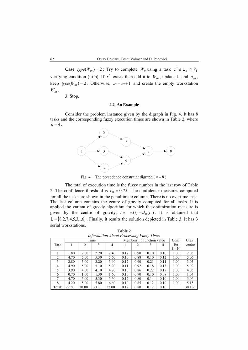
Consider the problem instance given by the digraph in Fig. 4. It has 8

tasks and the corresponding fuzzy execution times are shown in Table 2, where . 4=k

Fig. 4 − The precedence constraint digraph ( 8=n ).

The total of execution time is the fuzzy number in the last row of Table 2. The confidence threshold is .75.00 =c The confidence measures computed for all the tasks are shown in the penultimate column. There is no overtime task. The last column contains the centre of gravity computed for all tasks. It is applied the variant of greedy algorithm for which the optimization measure is given by the centre of gravity, i.e. )()( 0 itdiw = . It is obtained that

. Finally, it results the solution depicted in Table 3. It has 3 serial workstations.

{ 6,1,3,5,4,7,2,8=L }

Table 2 Information About Processing Fuzzy Times Time Membership function value

Task 1 2 3 4 1 2 3 4 Conf.

for C=10

Grav. centre

1 1.80 2.00 2.20 2.40 0.12 0.90 0.10 0.10 1.00 2.03 2 4.70 5.00 5.30 5.60 0.10 0.88 0.10 0.12 1.00 5.06 3 2.80 3.00 3.20 3.40 0.12 0.90 0.21 0.11 1.00 3.05 4 4.90 5.00 5.10 5.20 0.11 0.92 0.18 0.13 1.00 5.02 5 3.90 4.00 4.10 4.20 0.10 0.86 0.22 0.17 1.00 4.03 6 0.70 1.00 1.30 1.60 0.10 0.90 0.10 0.08 1.00 1.04 7 4.70 5.00 5.30 5.60 0.12 0.80 0.14 0.10 1.00 5.06 8 4.20 5.00 5.80 6.60 0.10 0.85 0.12 0.10 1.00 5.15

Total: 29.30 30.00 30.80 32.00 0.12 0.80 0.12 0.10 − 30.186


Table 3 Solution Structure for 10=C and 75.00 =c

Workstation fuzzy time Membership function value Work station

Tasks flow in workstation 1 2 3 4 1 2 3 4

Conf. for C=10

1 serial 1→2→3 9.6 10. 10.4 10.8 0.12 0.88 0.12 0.11 0.813 2 serial 4→5→6 9.9 10. 10.3 10.6 0.11 0.86 0.17 9.1 0.782 3 serial 7→8 9.7 10. 10.8 11.4 0.12 0.8 0.12 0.1 0.807

Consider now the case when 2.5=C and 8.00 =c . This time

1)( =≤ CtConf i , for , 6,5,4,3,1=i 82.0)( 2 =≤ CtConf , but

81.0) =≤ C( 8tConf79.0) =( 7 ≤ CtConf

)2( 7 =≤ CtConf. Therefore, task is an overtime task and since

the problem can be solved by creating a parallel workstation containing this overtime task. Applying the greedy algorithm it is obtained the solution described in Table 4.

71

Table 4

Solution Structure for 2.5=C and 8.00 =c Workstation fuzzy time Membership function value

Work station

Tasks flow in workstation

1

2

3

4

1

2

3

4

Conf. for

C=5.2 /10.4

1serial 1→3 4.6 5 5.2 5.6 0.12 0.90 0.21 0.10 0.92 2 serial 2 4.7 5.0 5.3 5.6 0.10 0.88 0.10 0.12 0.82 3 serial 4 4.9 5.0 5.1 5.2 0.11 0.92 0.18 0.13 1

4 parallel 5→6→7 9.7 10 10.2 10.8 0.12 0.80 0.17 0.10 0.92 5 serial 8 4.2 5.0 5.8 6.6 0.10 0.85 0.12 0.10 0.81

The solution has one parallel workstation and the number of virtual

serial stations is . From the last column in Table 4, we obtain that the confidence of the solution is (better that

6=vm81.0 8.00 =c ). The optimality of this

solution is proved by the fact that the computed value of the lower bound is . 6=Fm

5. A Hybrid Genetic Algorithm for ALB with Fuzzy Overtime Tasks

In this section, the main features of the GA [14], [20] for solving the

ALB problem with fuzzy overtime tasks are presented. Chromosome representation. The individuals in the populations are

represented as permutations of V , ),...,( 1 nvvv = that sort V in topological order [Knu76], i.e. implies Avv sr ∈),( sr < . From a technical point of view, such a permutation represents the assembly flow. This flow corresponds to many solutions having either different numbers of workstations or different internal structure. The task of computing the optimal solution corresponding to this flow is accomplished by the fitness function.


Population management. The initial population is obtained by generating random topological sorting. This is done by introducing random choices in the classical topological sorting algorithm described in [19]. It was proven that it ensures a good variability of the initial individuals.

The lifetime of an individual is the number of stages elapsed between it’s including in population and the moment when it is removed although this individual could have the best performance. The lifetime follows a truncated Gauss distribution )1,(μN . Taking larger values of the average lifetime of individuals prevents the depopulation μ . Reasonable values for μ are in the range . The main advantage of using predetermined lifetime duration is the preventing of stagnation. Its role is also important in selecting the potential parents for the crossover process. A drawback of predetermined lifetime is the rare occurrence of the total depopulation when the population size is too small or the lifetime is too short. A simple remedy is to activate the procedure for generating initial population.

}3/,...,5/{ nn

The population size is a periodic function depending on the evolution stage and within each period it follows a Fibonacci sequence with two initial values. The size of the period T depends on a prescribed maximum number of individuals. At the end of each evolution stage the individuals are sorted in the increasing order of the number of workstations. For the same number of workstations, the individuals are sorted in the decreasing order of the resulted confidence. The first individual in this list is the best within current population because it reaches the maximum confidence values for the minimum number of workstations. After updating the lifetime of individuals, the loosing life chromosomes are removed from the population, but those individuals having the minimum number of workstations among the removed ones are stored in a so-called thesaurus. This thesaurus also contains the best individuals extracted from the population in the last evolution stage. Finally, the best solutions (with respect both number of workstations and the confidence) are recuperated from the thesaurus. If the population remained after updating the lifetime exceeds the population size for the next stage then only the chromosomes in the front of the above list are preserved for the future.

Mutation. The individual suffering the mutation is randomly selected from the whole current population with the probability mπ . It is proposed a powerful mutation operator acting on a given chromosome ),...,( 1 nvvv = in the following way. A vertex is randomly selected, where hv },...,1{ nh∈ and it is made an attempt to move it to a different position. Since represents a topological sorting, the predecessors and successors of v are placed before and after , respectively. If is the rightmost predecessor of and is the leftmost successor of and either

v

hv rvh

hv lv

hv 1−< hl or 1+> hr then the mutation is successful (in the opposite case, the next mutation attempt is made). If


lhhr −>− then task moves to position hv 1−r and the sequence shifts leftwards one position. If 11 ,..., −+ rh vv hrlh −≥− then task moves to

position and the sequence shifts rightwards. The reason to move task to the furthest position is to maximize the Hamming distance between the initial chromosome and its mutant. This favours a better variability of the individuals. Let use denote by

hv1+lv

1−1,...,+ hl vv

)(v

h

μ the returned chromosome after the mutation of v . The resulted permutation )(vμ preserves the topological order and therefore no repair technique is needed. It was experimentally proved that this mutation operator ensures enough variability in the population even for a medium cardinality of V . For large instances, in order to ensure a high variability of the population, it was adopted the recurrent variant of the operator μ , by generating a random number }10/,..., n1{r∈ and computing ,

where ,

)(vrμ='v

))v(( 1j−= μμ)v(jμ r,...,1j = . A detailed investigation of the performance of this extended operator is published in [8].

Crossover. The number of crossovers to be accomplished during a given stage is determined so that the current population size, the number of successful mutations and the number of children do not exceed the maximum population size. The selection of potential parents is described below. As soon as a new chromosome is included in the evolution process, its individual affinity is defined by the resulted confidence divided by the product between the number of workstations and its lifetime. During the crossover process the mutual affinity of the individuals and is defined as

, where represents the Hamming distance between and . All pairs of individuals are sorted in the decreasing order of the mutual affinity. A given number of pairs from the front of this list effectively produce children. Therefore the individuals having a good performance concerning both the number of workstations and the confidence and being different enough, have a high chance to produce offsprings. This chance increases as the lifetime decreases. The mutation is done with the many points crossover operator, namely the crossover operator randomly splits two chromosomes into a number of parts. Each offspring is obtained by taking the first part from one parent and alternating then the parts of both parents, so that each task appears just once. The proposed genetic operators preserve the topological sorting property. This improves the method given [1], where the mutation is never considered due to the missing of an appropriate operator. In order to respect the desired cycle time, the method presented in [13] applies a repair technique to the offspring, while this approach does not.

v

(vaff

)(vaff

_) ind=

_

v

ind

,(_ vaffmutv

)'v'v

,(*)' vH'v

(_ vaffindv

*)' )',( vvH

Search stopping. The evolution ends when the maximum number of iterations is reached or there is no improvement of at least one of the objectives for a percentage of the evolution horizon.

Fitness function. The fitness function is applied to a chromosome and


returns two basic attributes that are the main and secondary objectives of the optimisation. The first attribute is the number of workstations. The second one is the resulted confidence, which is computed as the minimum among the confidences of the corresponding workstations. As it was stated in Section 2.2, our main goal is to find a solution with a minimum number of workstations, but whenever many such solutions exist the best is considered to be that solution having the higher confidence. The algorithm computing these two attributes is based on a greedy approach that extends the workstation under construction in the flow direction as long as the condition (3) remains true. Actually, the fitness function is computed as a particular case of the greedy method described in section 4.1, namely when it acts on a Hamiltonian path.

Grafting the greedy algorithm. This is done by running the greedy method at the beginning of the evolution and sending its output to the initial population. The second type of hybridisation is done differently from the case of the serial stations. Two indexes of workstations are randomly chosen on the current chromosome so that their difference does not exceed , where is the number of real workstations of the chromosome. The greedy method for parallel workstations is then applied to the tasks forming the stations between these cutting points.

5/m m

6. Performance Analysis

The experimental investigation was focused to the solving some

difficult instances of ALB with fuzzy overtime tasks. These problem instances have been obtained considering precedence digraphs with 30,111 and 121 tasks. So, the following instances have been considered in the experiment: LUTZ1.IN2 with 32 tasks with fuzzyfied times and 9 values for the cycle time, an example from the clothing industry with 5 values for the cycle time and ARCUS111.IN2 with 111 fuzzy times tasks and 9 values for C. The confidence threshold considered for all these examples was { }1,97.0,95.0,93.00 ∈c . For each problem instance, all defuzzification rules have been applied, so we finally obtained 4800 solutions. Five runs have been executed for each such problem instance.

For a given solution the following attributes were analyzed:

Fv mmerabs −=_ (absolute error) ( ) FFv mmmerrel /_ −= (relative error)

)*/()(1

Cmtdeff v

n

iii ∑

=

= (efficiency),

where the virtual number of workstation corresponding to the best solution given by the hybrid algorithm and the lower bound are defined as in the previous section. The denominator appearing in definition of efficiency

vm

Fm


represents a defuzzyfication operator applied to the total fuzzy time, and it is the same operator used by the greedy algorithm as an optimization measure for the corresponding problem instance. Observe that if denotes the minimal value of , then since we have that and

id

*m

vm −m Fmm ≥*Fv mmm −≤*

( ) ( ) FFvv mmmmmm −≤− ** . Actually, and are upper bounds of the real absolute and relative error, respectively. The advantage of using these bounds is the easier way the compute as compared to the

computational complexity (or rather impossibility) to obtain . The last column in Table 5 contains the values of the attribute representing the percentage of solutions whose optimality was detected using the optimality test.

erabs _ errel _

*mopt

Fm

Table 5

Performance of the Defuzzification Rules rule value abs_er rel_er eff opt

Min. 0.000 0.000 0.760 Av. 2.752 0.120 0.887

the center of gravity method Max. 5.000 0.290 0.940

0.005%

Min. 1.000 0.060 0.770 Av. 2.734 0.125 0.883

maximum

Max. 5.000 0.290 0.940

0.0%

Min. 1.000 0.060 0.770 Av. 2.711 0.123 0.884

mean of maximum

Max. 5.000 0.290 0.940

0.0%

Min. 1.000 0.060 0.540 Av. 2.688 0.124 0.618

weighted maximum

Max. 5.000 0.290 0.660

0.0%

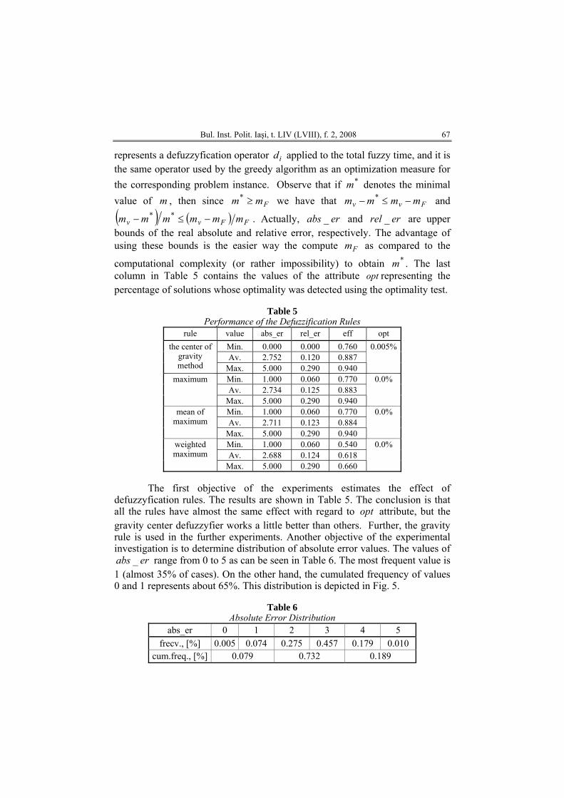
The first objective of the experiments estimates the effect of

defuzzyfication rules. The results are shown in Table 5. The conclusion is that all the rules have almost the same effect with regard to opt attribute, but the gravity center defuzzyfier works a little better than others. Further, the gravity rule is used in the further experiments. Another objective of the experimental investigation is to determine distribution of absolute error values. The values of

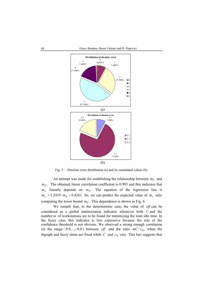
range from 0 to 5 as can be seen in Table 6. The most frequent value is 1 (almost 35% of cases). On the other hand, the cumulated frequency of values 0 and 1 represents about 65%. This distribution is depicted in Fig. 5.

erabs _

Table 6

Absolute Error Distribution abs_er 0 1 2 3 4 5

frecv., [%] 0.005 0.074 0.275 0.457 0.179 0.010 cum.freq., [%] 0.079 0.732 0.189


Distribution of absolute error

345.700%

00.005%5

1.000%1

7.400%

227.500%

417.900%

012345

(a)

Distribution of absolute error4, 5

18.900%0, 1

7.900%

2, 373.200%

0, 12, 34, 5

(b)

Fig. 5 − Absolute error distribution (a) and its cumulated values (b).

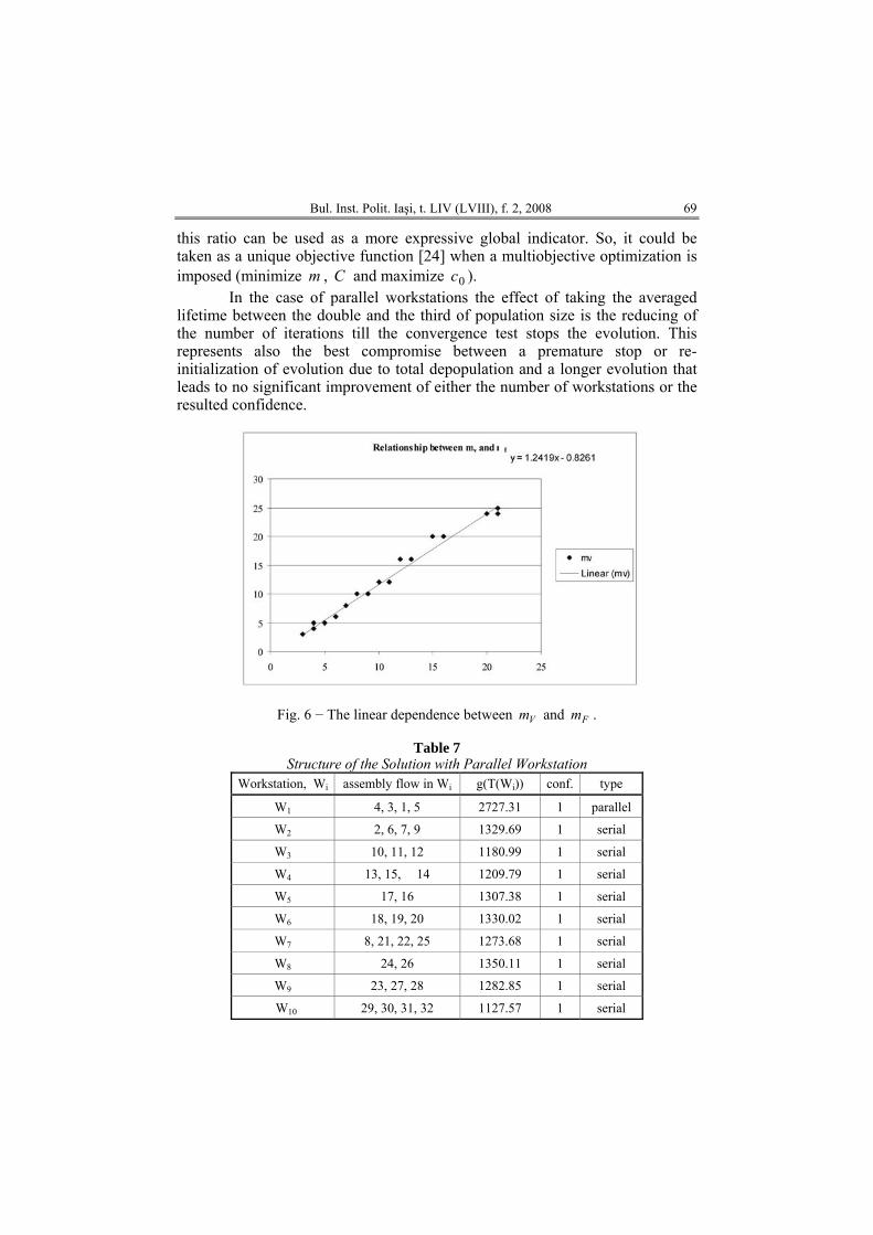
An attempt was made for establishing the relationship between and

. The obtained linear correlation coefficient is 0.993 and this indicates that linearly depends on . The equation of the regression line is

Vm

Fm

vm Fm8261.02419.1 +⋅= Fmym . So, we can predict the expected value of only

computing the lower bound . This dependence is shown in Fig. 6. vm

FmWe remark that, in the deterministic case, the value of can be

considered as a global minimization indicator whenever both C and the number m of workstations are to be found for minimizing the total idle time. In the fuzzy case, this indicator is less expressive because the role of the confidence threshold is not obvious. We observed a strong enough correlation (in the range ) between and the ratio , when the digraph and fuzzy times are fixed while C and vary. This fact suggests that

eff

8.0,...,9.0 −− eff 0/ cmC

0c


this ratio can be used as a more expressive global indicator. So, it could be taken as a unique objective function [24] when a multiobjective optimization is imposed (minimize , and maximize ). m C 0c

In the case of parallel workstations the effect of taking the averaged lifetime between the double and the third of population size is the reducing of the number of iterations till the convergence test stops the evolution. This represents also the best compromise between a premature stop or re-initialization of evolution due to total depopulation and a longer evolution that leads to no significant improvement of either the number of workstations or the resulted confidence.

Fig. 6 − The linear dependence between and . Vm Fm

Table 7

Structure of the Solution with Parallel Workstation Workstation, Wi assembly flow in Wi g(T(Wi)) conf. type

W1 4, 3, 1, 5 2727.31 1 parallel

W2 2, 6, 7, 9 1329.69 1 serial

W3 10, 11, 12 1180.99 1 serial

W4 13, 15, 14 1209.79 1 serial

W5 17, 16 1307.38 1 serial

W6 18, 19, 20 1330.02 1 serial

W7 8, 21, 22, 25 1273.68 1 serial

W8 24, 26 1350.11 1 serial

W9 23, 27, 28 1282.85 1 serial

W10 29, 30, 31, 32 1127.57 1 serial


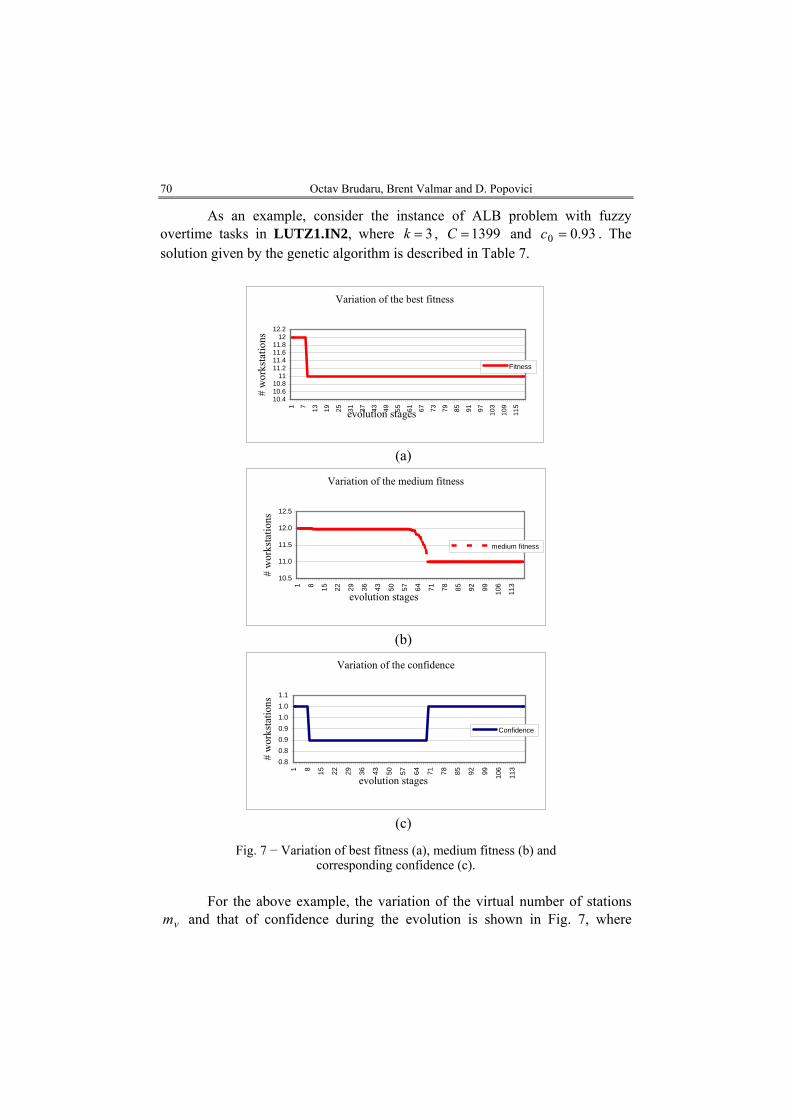
As an example, consider the instance of ALB problem with fuzzy overtime tasks in LUTZ1.IN2, where 3=k , 1399=C and 93.00 =c . The solution given by the genetic algorithm is described in Table 7.

Variation of the best fitness

10.410.610.8

1111.211.411.611.8

1212.2

1 7 13 19 25 31 37 43 49 55 61 67 73 79 85 91 97 103

109

115

evolution stages

# w

orks

tatio

ns

Fitness

(a)

Variation of the medium fitness

10.5

11.0

11.5

12.0

12.5

1 8 15 22 29 36 43 50 57 64 71 78 85 92 99 106

113

evolution stages

# w

orks

tatio

ns

medium fitness

(b)

Variation of the confidence

0.80.80.90.91.01.01.1

1 8 15 22 29 36 43 50 57 64 71 78 85 92 99 106

113

evolution stages

# w

orks

tatio

ns

Confidence

(c)

Fig. 7 − Variation of best fitness (a), medium fitness (b) and corresponding confidence (c).

For the above example, the variation of the virtual number of stations

and that of confidence during the evolution is shown in Fig. 7, where vm


1399=C and . 8.00 =c

Variation of the medium fitness

10 19 28 37 46 55 64 73 82 91 100

109

118

127

136

145

154

evolution stages

10.5

11.0

11.5

12.0

12.51

# w

orks

tatio

ns medium fitness

(a)

Variation of the confidence

0.920

0.940

0.960

0.980

1.000

1.020

1 6 11 16 21 26 31 36 41 46 51 56 61 66 71 76 81 86

evolution stages

# w

orks

tatio

ns

confidence

(b)

Variation of the smoothing attribute

0

0.1

0.2

0.3

0.4

0.5

1 10 19 28 37 46 55 64 73 82 91 100

109

118

127

136

145

154

evolution stages

# w

orks

tatio

ns

smoothing factor

(c)

Fig. 8 − Variation of medium fitness (a), confidence (b) and smoothing factor (c) in the case of parallel stations.

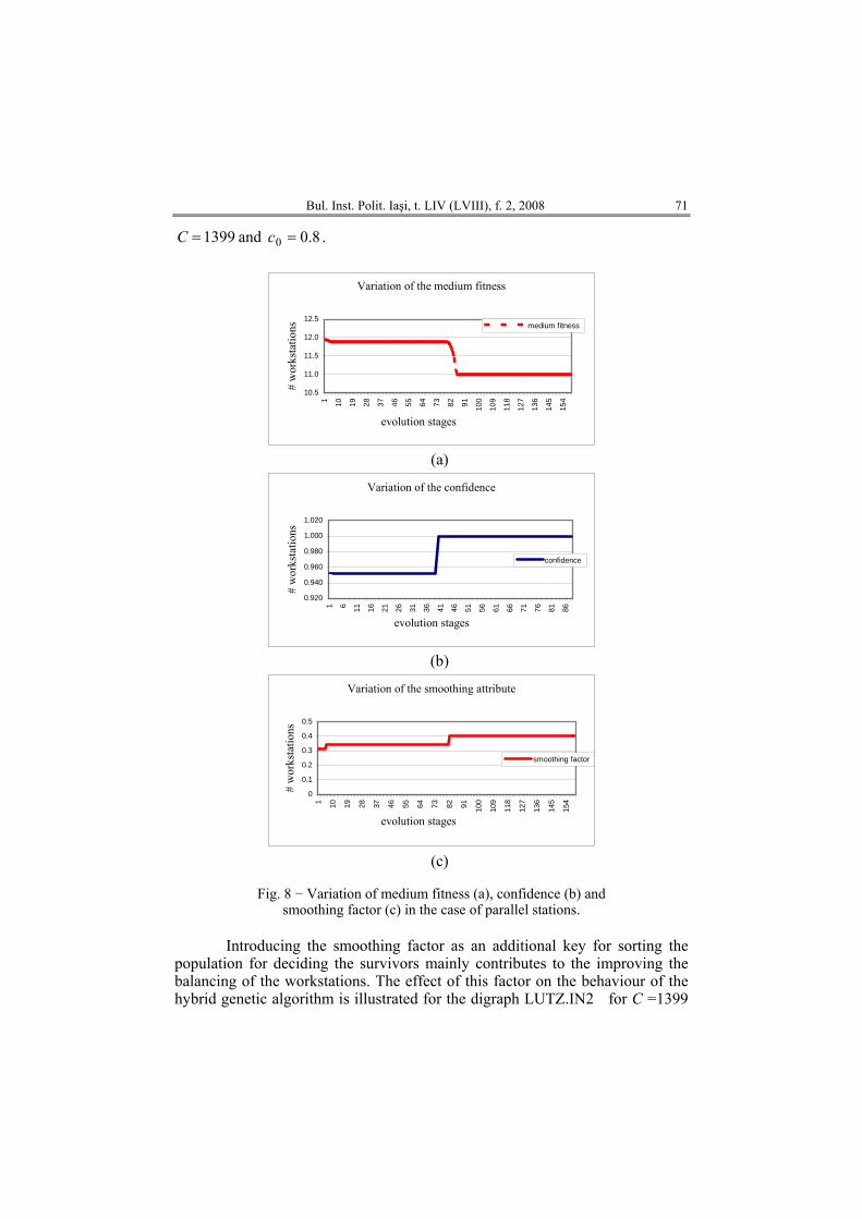
Introducing the smoothing factor as an additional key for sorting the

population for deciding the survivors mainly contributes to the improving the balancing of the workstations. The effect of this factor on the behaviour of the hybrid genetic algorithm is illustrated for the digraph LUTZ.IN2 for C =1399


and in Fig. 8. 8.00 =cWe conclude that the proposed genetic algorithm hybridized with the

greedy method for solving of the assembly line balancing with parallel stations has a good performance concerning the optimality of the found solutions.

7. Conclusions and Further Research

This paper presented a fuzzy model for assembly line balancing problem with parallel workstations. The greedy algorithm proposed for solving this problem was analyzed with regard to multiple performance criteria. It was obtained the best defuzzyfication rule to be used as optimization measure. An optimality detecting test was extended to the case of fuzzy times and parallel workstations. The greedy method was grafted on a genetic algorithm. The performance of the resulted hybrid algorithm was experimentally analyzed and it was observed a linear dependency between the value of the lower bound given by the optimality criterion and the virtual number of workstations given by the proposed algorithm. The proposed algorithm can be easily extended for handling any multiple of the cycle time.

Received: June 10, 2008 “Gheorghe Asachi” Technical University of Iaşi,

Department of Management and Production Systems Engineering

e-mail: [email protected] and

*Institute for Computer Science, Romanian Academy Iaşi Branch

R E F E R E N C E S

1. Ajenbit A., Debora A., Wainwright R.L., Applying Genetic Algorithms to the U-

Shaped Assembly Line Balancing Problem. Mathematical and Computer Science Department, The University of Tulsa, USA, 2000.

2. Askin R.G., Standridge C.R., Modelling and Analysis of Manufacturing Systems. John Wiley & sons Inc., 1993.

3. Baybars I., A Survey of Exact Algorithms for the Simple Assembly Line Balancing. Management Science, 32, 909-032, 1986.

4. Boothroyd G., Assembly, Automation and Product Design. Marcel Decker Inc., 1998. 5. Bourrieres J.P., Contribution à la modélisation integrée des systemes robotisés

d’assemblage. Thése no. 240, l’u. F.R. des Sciences et des Techniques de l’Université de Franche – Conté, 1990.

6. Brudaru O., Belous V., Assembly Line Balancing with Fuzzy Execution Times. in: Proceedings of EUFIT’96 - Fourth European Congress on Intelligent Techniques and Soft Computing, Aachen, Germany, September 2-5, Vol. 3, Verlag Mainz, 1996, 1966-1971.

7. Brudaru O., Belous V., Rusu C., Assembly Line Balancing with Fuzzy Execution Times and Mixed Models. in: Proceedings of ISFL’97 - Second International

mailto:[email protected]


Symposium on Fuzzy Logic and Application, Zurich, February 12-14, 1997, 158-164.

8. Brudaru O., Curteanu M., Copăceanu C.M., Valmar B., A Mutation Operator Preserving the Topological Sorting. Bul. Instit. Politehnic, Iaşi, VIII, 1-2, 2003.

9. Brudaru O., Copăceanu C.M., Valmar B., Assembly Line Balancing Paradigm: Achievements and New Trends. New Trends in Computer Science and Engineering (anniversary volume), M. Craus, D. Gâlea, A. Valachi (Eds.), Department of Computer Engineering, Faculty of Automatic Control and Computer Engineering, “Gheorghe Asachi” Technical University, POLIROM Press, Iaşi, 2003, 187-218.

10. Brudaru O., Megson G.M., An Approximation Algorithm for Assembly Line Balancing with Parallel Workstations. The 11th international DAAAM Symposium “Intelligent Manufacturing & Automation: Man – Machine – Nature”, 19-21st October 2000, Wien, Austria.

11. Brudaru O., Valmar B., Copăceanu C.M., Assembly Line Balancing Paradigm: Achievements and New Trends. New Trends in Computer Science and Engineering (anniversary volume), D. Gâlea (Eds.), Department of Computer Engineering, Faculty of Automatic Control and Computer Engineering, “Gheorghe Asachi” Technical University, POLIROM Press, Iaşi, 2003, 187-218.

12. Buxey G.M., Assembly Line Balancing with Multiple Station. Management Science, Vol. 20, 6, 1010-1021, 1974.

13. Delchambre A., Falkenauer E., Rekiek B., The Grouping Genetic Algorithm: An Efficient Method to Design Assembly Lines. in Computer-aided process and assembly planning: methods, tools and technologies, Gordon and Breach, 1998.

14. Goldberg D.E., Genetic Algorithms in Search, Optimization and Machine Learning. Addison – Wesley Publishing Co., Inc., 1989.

15. S. Gou J.L, High-Speed Analogue Fuzzy Logic Controller. R. Oldenbourg Verlag, Munchen, 1995.

16. Gutjahr A., Nemhauser G., An Algorithm for the Line Balancing Problem. Management Science, Vol. 11, 2, 1964, 308-315.

17. Hirota T., A Digital Representation of Fuzzy Numbers and its Application. Proceedings of IIZUKA'90, 1990, 527-529.

18. Kao E.P.C., A Preference Order Dynamic Program for Stochastic Assembly Line Balancing. Management Science, Vol. 22, 10, 1976, 1097-1104.

19. Knuth D.E., The Art of Computer Programming. Technical Publishing House, 1976, Bucharest (in Romanian).

20. Michalewicz Z., Genetic Algorithms + Data Structures = Evolution Programs. Springer Verlag, Berlin, 1992.

21. Robert L., Carraway A., A Dynamic Programming Approach to Stochastic Assembly Line Balancing. Management Science, Vol. 4, 1989, 459-472.

22. Salverson M., The Assembly Line Balancing Problem. Trans. of A.S.M.E. Vol. 77, 1955.

23. Scholl A., Balancing and Sequencing of Assembly Lines. Contribution to Management Science, Second Edition, Phisica-Verlag Heilderberg, A Springer-Verlag Company, Printed in Germany (1999).

24. Slany W., Fuzzy Scheduling. in: CD-Technical Report 94/66,Christian Doppler for


Expert Systems, Technical University Wien, Wien (1994). 25. Sniedovici M., Analysis of a Preference Order Assembly Line Problem.

Management Science, Vol. 27, 9, 1981, 1067-1081. 26. Talbot F.B., A Comparative Evaluation of Heuristic Line Balancing Technique.

Management Science, Vol. 32, 4, 1986, 430-454. 27. Tsujimura Y., Gen M., Li Y., Kubotta E., An Efficient Method for Solving Fuzzy

Assembly Line Balancing Problem Using Genetic Algorithm. Proceedings of the Third European Congress on Intelligent Techniques and Soft Computing, Aachen, Germany, August 28-31, 1995, Vol. 1, Verlag Mainz, 406-415 (1995).

ALGORITM GENETIC HIBRID PENTRU ECHILIBRAREA LINIILOR DE

ASAMBLARE CU TIMPI FUZZY ŞI STAŢII PARALELE

(Rezumat)

Se abordează problema echilibrării liniilor de asamblare în care timpii de execuţie pentru faze sunt numere fuzzy având ca obiectiv minimizarea numărului de staţii de lucru. Este definită o margine inferioară pentru numărul de staţii şi este prezentată o tehnică de căutare binară pentru calculul acesteia. Este propusă o metodă greedy şi apoi un algorithm genetic pe care este grefată metoda greedy prin inserarea în populaţia iniţială a soluţiei oferite cât şi prin includerea metodei greey într-un operator de hipermutaţie. Sunt analizate experimental performanţele algoritmului genetic hibrid cu privire la optimalitatea soluţiilor oferite folosind instanţe speciale de dificultate recunoscută. Abordarea propusă în lucrare oferă performanţe foarte bune atât cu privire la calitatea soluţiilor, cât şi relativ la timpul de calcul necesar.

HYBRID GENETIC ALGORITHM FOR ASSEMBLY LINE BALANCING … Brudaru(ac. 2).pdf · HYBRID GENETIC...

Documents

Transcript of HYBRID GENETIC ALGORITHM FOR ASSEMBLY LINE BALANCING … Brudaru(ac. 2).pdf · HYBRID GENETIC...