Codul de practici si proceduri al autoritatii de marcare temporala ...
Revista Română de Statistică - Supliment nr. 5 / 2019
SUMAR / CONTENTS 5/2019REVISTA ROMÂNĂ DE STATISTICĂ SUPLIMENT
MODELUL GRAVITAȚIONAL UTILIZAT ÎN ANALIZELE ECONOMICE 3THE GRAVITATIONAL MODEL USED IN THE ECONOMIC ANALYZES 21Prof. Constantin ANGHELACHE PhDProf. Gabriela Victoria ANGHELACHE PhDAssoc. Mădălina-Gabriela ANGHEL PhD Gabriel-Ștefan DUMBRAVĂ PhD StudentOana-Ana-Maria SIMA Master Student
THE ANALYSIS OF MACRO-STABILIZATION OF THE FINANCIAL-BANKING SYSTEM 39György BODÓ PhD Student
MODEL DE ANALIZĂ A COMPORTAMENTULUI SOCIETĂȚILOR ÎN PERIOADA POST-CRIZĂ 48ANALYSIS MODEL OF THE POST-CRISIS BEHAVIOR OF THE COMPANIES 56Ștefan Virgil Iacob PhD
STATIC AND STRUCTURAL ANALYSIS OF GROSS DOMESTIC PRODUCT 64Tudor SAMSON Ph.D Student Alexandra PETRE (OLTEANU) PhD Student Cristian OLTEANU PhD StudentMarin-Marius GĂNCIULESCU Master Student
MIGRAȚIA ECONOMICĂ – ANALIZA FACTORILOR DETERMINANȚI AI ACESTEIA 73THE ECONOMIC MIGRATION - ANALYSIS OF ITS DETERMINANTS 83Olivia –Georgiana NIȚĂ PhD Student Alexandru BADIU PhD Student
THE BASEL AGREEMENTS – THE ANALYSIS OF THE BANKING RISKS 93Prof. Gabriela Victoria ANGHELACHE PhDGyörgy BODÓ PhD Student Radu STOICA PhD StudentDaniel GHERASIM Master Student
www.revistadestatistica.ro/supliment

Romanian Statistical Review - Supplement nr. 5 / 20192
ASPECTE TEORETICE PRIVIND ELABORAREA PREVIZIUNILOR MACROECONOMICE 100THEORETICAL ASPECTS REGARDING THE ELABORATION OF THE MACROECONOMIC FORECASTS 111Emilia STANCIU PhD Student Marius POPOVICI PhD Student Alexandra PETRE (OLTEANU) PhD Student Andreea-Ioana MARINESCU PhDGabriela Iuliana CARAIANI Master Student
THE ANALYSIS OF THE FIRM BASED ON THE STATISTICAL INDICATORS 121Prof. Radu Titus MARINESCU PhDDoina AVRAM PhD StudentCristian OLTEANU PhD Student Maria MIREA PhD Student

Revista Română de Statistică - Supliment nr. 5 / 2019 3
Modelul gravitaţional utilizat în analizele economice
Prof. univ. dr. Constantin ANGHELACHE ([email protected])
Academia de Studii Economice din București / Universitatea „Artifex” din București Prof. univ. dr. Gabriela Victoria ANGHELACHE([email protected])
Academia de Studii Economice din București
Conf. univ. dr. Mădălina-Gabriela ANGHEL([email protected])
Universitatea „Artifex” din București
Drd. Gabriel-Ștefan DUMBRAVĂ ([email protected])
Academia de Studii Economice din București Oana-Ana-Maria SIMA Master Student
Abstract Numeroase studii empirice au aratat ca fl uxurile comerciale urmeaza
principiile fi zicii referitoare la gravitatie: doua forte opuse determina nivelul
comertului bilateral intre tari, nivelul activitatii economice si a venitului,
pe de o parte si totalitatea barierelor afl ate in calea derularii comertului,
pe de alta parte. Acestea din urma includ: costurile cu transportul, politici
comerciale prohibitive, nesiguranta exportatorilor si importatorilor privind
evolutia diferitelor conditii de desfasurare a comertului cum ar fi evolutia
cursului valutar, diferentele culturale, existenta frontierelor nationale,
diversitatea preferintelor consumatorilor precum si diverse alte impedimente.
Analiza efectuată de autori evidențiază faptul că modelul gravitațional
asigură posibilitatea analizei comerțului internațional. Ecuațiile de tip
gravitațional au câteva caracteristici care asigură posibilitatea efectuării
studiilor empirice fi ind o ecuație bilaterală. Cu toate ca modelul gravitational
a avut, inca de la inceputurile utilizarii lui, un succes empiric care putea fi
cu difi cultate contestat, acest model a avut totusi parte, o perioada de timp,
si de critici care vizau lipsa unei fundamentari teoretice. Din acel moment a
fost din ce in ce mai mult acceptat faptul ca ecuatia gravitationala poate fi
extrasa pornind de la anumite ipoteze din modele teoretice, cum ar fi modele
ricardiene, modele de tip Heckscher-Ohlin sau modele de scara apartinand
Noi teorii a comertului international. Aceste trei tipuri de modele difera in
esenta prin modul in care este realizata specializarea produselor de catre
diferite tari.
Keywords: comerț internațional, regionalizare, import, export, curs
valutar, model gravitațional, modelul interlink. Classifi cation JEL: C50, F13, F40
Romanian Statistical Review - Supplement nr. 5 / 20194
Introduction Ecuatia gravitatiei este una dintre cele mai utilizate instrumente in studiile empirice privind problemele comertului international. Desi obiectivul principal al modelului gravitational este estimarea potentialului comercial pot fi mentionate si alte directii de utilizare ale acestui model cum ar fi : estimarea
costurilor pe care le implica frontierele dintre natiuni, explicarea evolutiei
ciclice a comertului international, identifi carea efectelor regionalizarii si nu
in ultimul rand explicarea efectului diferitelor variabile economice asupra
comertului cum ar fi spre exemplu, impactul pe care il are volatilitatea sau
evolutia cursului valutar asupra comertului s.a.m.d. Numarul variabilelor
explicative precum si varietatea formelor in care acestea sunt cuantifi cate au
cunoscut asemenea explozie in ultimii 20 de ani incat o simpla enumerare
a acestora devine destul de difi cila si risca sa fi e incompleta. Prin urmare,
in continuare este realizata o prezentare a celor mai importante utilizari ale
modelului gravitational impreuna cu variabilele cele mai semnifi cative fara a
avea pretentia unei prezentari complete.
Literature review Anghelache și Anghel (2018), precum și Corbare, Durlauf și
Hansen (2006) au analizat principalele metode și modele econometrice
utilizate în analizele economice. Anghelache (2008) a prezentat indicatorii
statistici aplicați în studiul comerțului international. O tema similară este
analizată de Anghelache și Anghel (2016). Anghelache, Mitruţ și Voineagu
(2013) au studiat aspecte fundamentale ale statisticii macroeconomice.
AnghelachePârţachi, Gonţa și Kralik (2012) au analizat elemente referitoare
la modelul gravitational. Arcidiacono și Miller (2011) au cercetat noțiuni
privind modelele dinamice. Benjamin, Herrard, Hanee-Bigot și Tavere (2010)
au analizat utilizarea modelelor econometrice în activitatea de previzionare.
Dascal, Mattas, Tzouvelekas (2002) au utilizat un model gravitațional în
vederea studiului infl uenței variației cursului valutar asupra comertului
exterior. Elliott, Müller și Watson (2015), precum și Phillips, Sun și Jin (2006)
au studiat aspecte ale testării modelelor econometrice. Johansen și Nielsen
(2010) s-au referit la inferența în cazul modelelor autoregresive. Müller (2007)
a studiat estimarea variațiilor de lungă durată. Newbold, Karlson și Thorne
(2010) au analizat elemente de bază ale statisticii economice. Pesavento și
Rossi (2006) au analizat aspecte ale eșantionării.
Metodologia cercetării Modelul gravitational pentru fl uxurile comerciale internationale isi
are originea in legea atractiei universale propusa de Newton (1687) care face
Revista Română de Statistică - Supliment nr. 5 / 2019 5
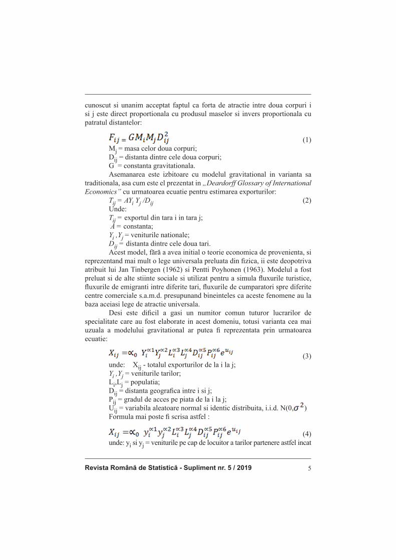
cunoscut si unanim acceptat faptul ca forta de atractie intre doua corpuri i
si j este direct proportionala cu produsul maselor si invers proportionala cu
patratul distantelor:
(1)
Mj = masa celor doua corpuri;
Dij = distanta dintre cele doua corpuri;
G = constanta gravitationala.
Asemanarea este izbitoare cu modelul gravitational in varianta sa
traditionala, asa cum este el prezentat in „Deardorff Glossary of International
Economics” cu urmatoarea ecuatie pentru estimarea exporturilor:
Tij = AYi Yj /Dij (2)
Unde:
Tij = exportul din tara i in tara j;
A = constanta;
Yi ,Yj = veniturile nationale;
Dij = distanta dintre cele doua tari.
Acest model, fără a avea initial o teorie economica de provenienta, si reprezentand mai mult o lege universala preluata din fi zica, ii este deopotriva atribuit lui Jan Tinbergen (1962) si Pentti Poyhonen (1963). Modelul a fost preluat si de alte stiinte sociale si utilizat pentru a simula fl uxurile turistice, fl uxurile de emigranti intre diferite tari, fl uxurile de cumparatori spre diferite centre comerciale s.a.m.d. presupunand bineinteles ca aceste fenomene au la baza aceiasi lege de atractie universala. Desi este difi cil a gasi un numitor comun tuturor lucrarilor de specialitate care au fost elaborate in acest domeniu, totusi varianta cea mai uzuala a modelului gravitational ar putea fi reprezentata prin urmatoarea ecuatie:
(3) unde: Xij - totalul exporturilor de la i la j; Yi ,Yj = veniturile tarilor; Li,Lj = populatia; Dij = distanta geografi ca intre i si j; Pij = gradul de acces pe piata de la i la j; Uij = variabila aleatoare normal si identic distribuita, i.i.d. N(0, ) Formula mai poste fi scrisa astfel : (4) unde: yi si yj = veniturile pe cap de locuitor a tarilor partenere astfel incat
Romanian Statistical Review - Supplement nr. 5 / 20196
Parametrii sunt in general estimati prin metoda celor mai mici patrate
pornind de la forma logaritmica a ecuatiei:
(5)
Metoda celor mai mici patrate nu este intotdeauna cea mai potrivita si
poate sa induca distorsiuni serioase in parametrii estimati datorita premiselor,
destul de restrictive, pe care se bazeaza aceasta metoda si care de multe ori nu
se mentin in conditii reale.
Ecuatiile de tip gravitational au cateva caracteristici care pot explica
succesul lor in studiile empirice. In primul rand, ecuatia gravitationala este
bilaterala. Ea explica variabila dependenta, de natura comertului exterior prin
combinarea unor variabile macroeconomice care descriu economia ambelor
tari partenere (marime, venit etc). Pe langa aceste marimi cu caracter bilateral
se adauga indicatorii privind costurile de transport intre cele doua tari si in
general variabile privind accesul pe piata.
In al doilea rand, ecuatia gravitatiei poate fi utilizata pentru a estima
atat factorii de volum cat si factorii privind natura fl uxurilor comerciale. Ultima situatie necesita introducerea unui indice al comertului intraindustrial ca variabila dependenta. Procentul comertului intraindustrial este in general determinat de similitudinea gradulul de inzestrare al tarilor partenere cu factori de productie care poate fi surprinsa si prin diferenta de venit pe cap de
locuitor dintre tari.
In al treilea rand, teoria ofera puternice temelii pentru un model bazat
pe indicatori cu grad redus de complexitate pentru care exista valori inregistrate
in cazul marii majoritati a tarilor si pe o perioada sufi cient de lunga. Aceasta
caracteristica este foarte utila atunci cand scopul este de a integra un numar
mare de tari in model iar baza de date statistice a acestora este limitata.
Modelul gravitational, data fi ind natura variabilelor independente, se
preteaza la analiza comertului international la un nivel ridicat de agregare.
Majoritatea modelelor au fost aplicate pe exporturile totale ale deferitelor tari.
Acest lucru nu exclude bineinteles utilizarea modelului gravitational pentru
date detaliate pe categorii de produse. Un exemplu recent este Gaulier si
Zignago (2004) care utilizeaza date cu un grad ridicat de detaliere pentru a
studia impactul factorilor de proximitate si al nivelului de specializare asupra
comertului.
Pornind de la un model de forma:

Revista Română de Statistică - Supliment nr. 5 / 2019 7
(6)
Unde:
α = constanta in timp si spatiu;
αt = efect fi x , specifi c fi ecarei perioade t si constant in plan teritorial;
αij - efect fi x, specifi c fi ecarei perechi ij si constant in timp;
PIBEit , PIBIjt = PIB-ul pe cap de locuitor al exportatorului respectiv
al importatorului;
PEi,,PIjt, = populatia exportatorului/importatorului;
Dij = distanta dintre cele doua tari;
εij = variabila aleatoare independenta si identic distribuita, de medie
1 si variatie constanta, i. i.d. (1,σ ) care prin logaritmare va deveni:
(7)
putem interpreta parametric β ca si elasticitati ale exportului functie
de factorii de infl uenta dupa rationamentul care urmeaza.
Prin diferentiere de gradul intai dupa variabila temporala t, ecuatia de
mai sus devine
(8)
Se cunoaste faptul ca diferenta logaritmilor aproximeaza ritmul de
crestere:
(9)
aproximarea fi ind cu atat mai puternica cu cat diferenta de la perioada
t-1 la perioada t este mai mica.
Prin urmare, coefi cientii βi i=1,4 arata modifi carea ritmului de
crestere al exporturilor la modifi carea cu 1 (100% in exprimare procentuala) a
ritmului de crestere in evolutia factorilor de infl uenta.
Pentru a obtine interpretarea coefi cientului β5, corespunzator unei
variabile pur teritoriale, se procedeaza in mod analog, insa de data aceasta
diferentele de ordinul intai se vor realiza in plan teritorial. Presupunem
ca perechile de tari ij sunt ordonate dupa un criteriu oarecare. Diferentele
perechilor consecutive pentru un an fi xat, t ar arata astfel:
Romanian Statistical Review - Supplement nr. 5 / 20198
(10)
Coefi cientul β5, va avea de aceasta data aceiasi interpretare ca si
ceilalti coefi cienti cu deosebirea cu variatia se manifesta in plan teritorial si
nu in plan temporal.
Ecuatia (6) nu poate fi estimata direct datorita coliniaritatii dintre
variabile teritoriale de distanta, Dij specifi ca fi ecarei perechi de tari si constanta
in timp si efectul fi x, specifi c fi ecarei perechi αij, ambele avand prin urmare
aceleasi proprietati si aceiasi variatie in profi l teritorial. Prin urmare, vom
inlatura alternativ cele doua variabile.
· Model de analiza structurii comertului international Suprapunerile comerciale (import si export in aceiasi industrie) sunt
examinate de Bergstrand (1989) si Hummels si Levinsohn (1995). Acestia
au construct indici comerciali bilaterali la nivel industrial in ceea ce priveste
comertul intra-industrial. Acesti indicatori sunt agregati la nivel national si
media ponderata a acestora este explicata folosind o ecuatie gravitationala.
O metoda alternativa utilizata pentru a diferentia comertul inter-industrial de
fl uxurile comerciale intra-industriale este explicat in Fontagne, Freudenberg
si Peridy (1998). In lucrarile amintite anterior se estimeaza ponderile in total
comert a tipurilor de comert diferentiindu-se in acest fel de marea majoritate
a modelelor de tip gravitational care estimeaza in general volumul total al
vanzarilor la extern.
Doua lucrari de data recenta care se inscriu pe aceasta linie sunt
Kandogan (2004) si (2004). In ultima lucrare este aratat faptul ca variabilele
explicative au efecte diferite asupra diferitelor componente ale comertului
exterior si ca pe masura ce economiile a doua tari si inzestrarea cu factori de
productie devine din ce in ce mai similara, volumul comertului intra-industrial
orizontal creste. In modelul specifi cat pentru comertul total variabilele sunt
introduse in forma logaritmata:
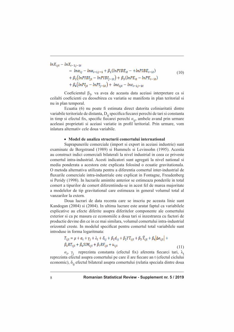
(11)
αi, γj reprezinta constanta (efectul fi x) aferenta fi ecarci tari, λt
reprezinta efectul asupra comertului pe care il are fi ecare an t (efectul ciclului
economic), δij efectul bilateral asupra comertului (relatia speciala dintre doua
Revista Română de Statistică - Supliment nr. 5 / 2019 9
tari care nu este surprinsa de variabilele explicative), iar celelalte variabile care
apar in model, in ordinea corespunzatoare sunt: distanta, productia cumulata
a celor doua tari, productia medie pe cap de locuitor, variatia absoluta a ratei
reale de schimb, rezerva valutara totala, similaritatea tarilor si diferenta de
inzestrare cu factori de productie. Ultimele doua variabile vor fi prezentate
in detaliu in cele ce urmeaza deoarece nu sunt direct observabile din datele
statistice ofi ciale.
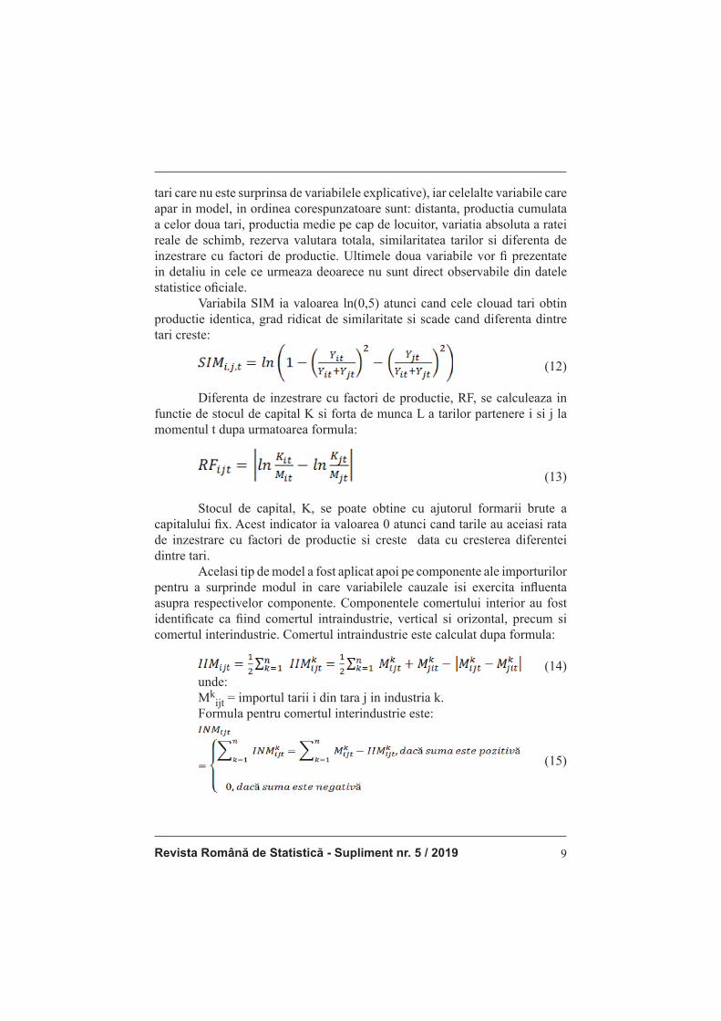
Variabila SIM ia valoarea ln(0,5) atunci cand cele clouad tari obtin
productie identica, grad ridicat de similaritate si scade cand diferenta dintre
tari creste:
(12)
Diferenta de inzestrare cu factori de productie, RF, se calculeaza in
functie de stocul de capital K si forta de munca L a tarilor partenere i si j la
momentul t dupa urmatoarea formula:
(13)
Stocul de capital, K, se poate obtine cu ajutorul formarii brute a
capitalului fi x. Acest indicator ia valoarea 0 atunci cand tarile au aceiasi rata
de inzestrare cu factori de productie si creste data cu cresterea diferentei
dintre tari.
Acelasi tip de model a fost aplicat apoi pe componente ale importurilor
pentru a surprinde modul in care variabilele cauzale isi exercita infl uenta asupra respectivelor componente. Componentele comertului interior au fost identifi cate ca fi ind comertul intraindustrie, vertical si orizontal, precum si
comertul interindustrie. Comertul intraindustrie este calculat dupa formula:
(14)
unde:
Mkijt = importul tarii i din tara j in industria k.
Formula pentru comertul interindustrie este:
(15)

Romanian Statistical Review - Supplement nr. 5 / 201910
Importurile intraindustrie orizontale pot fi defi nite ca fi ind importurile
intraidustrie cu acelasi tip de produse p:
(16)
Unde:
Mkpijt = reprezinta importurile in tara i din tara j pentru produsul p din
industria k la momentul t.
Importul intraindustrie vertical, adica comertul in aceiasi industrie dar
cu produse diferite sau produse cu diferite grade de prelucrare, se calculeaza
astfel:
(17)
· Estimarea efectelor regionalizarii in comertul international Modelele gravitationale au fost utilizate in sens larg pentru a evalua
infl uenta masurilor de politica comerciala asupra fl uxurilor comerciale si in special infl uenta acordurilor de integrare regionala. Daca consideram exemplul a doua tari intre care s-a incheiat un acord de integrare regionala poate fi introdusa o variabila alternativa care ia valoarea 1 daca cele doua tari
se afl a la un momentul t in acord bilateral si 0 in caz contrar. Daca parametrul estimat al variabilei alternative este pozitiv si semnifi cativ atunci se poate
trage concluzia ca regionalizarea creeaza fl uxuri comerciale . Aceasta estimare poate fi facuta cu scopul de a simula potentialul comercial corespunzator
oricarei variante de integrare regionala intre diferite grupe de tari.
Un exemplu de model pentru care ia in considerare cele mai
importance acorduri regionale printre care si Uniunea Europeana este cel
utilizat de Soloaga si Winters (2001). Modelul utilizat ia in considerare pe
langa variabile traditionale si variabile alternative de genul celor amintite
anterior. Ecuatia testata empiric pe importurile a 58 de tari pe perioada 1980-
1996 este:
(18)
Valoarea importurilor tarii i din tara j sunt explicate in functie de PIB,
populatie, doua variabile de distanta, suprafata tarilor, variabile alternative
Revista Română de Statistică - Supliment nr. 5 / 2019 11
pentru existenta frontierei comune, tara insulara sau continentala si
proximitate culturala (limba comuna). Aceste variabile comune diferitelor
modele estimeaza volumul importurilor independent de existenta politicilor
regionale. Pe langa aceste variabile sunt introduse si variabile specifi ce prin
care se estimeaza efectele regionalizarii. Pk reprezinta o variabile alternativa
care ia valoarea 1 daca tara i sau j este participanta la acordul k, coefi cientul
bk arata cu cat este mai mare comertul daca ambele tari fac parte din acordul
k, coefi cientul mk arata cu cat sunt mai mari importurile tarii i care face parte
din acord fata de toti partenerii sai comerciali iar coefi cientul nk arata cu cat
sunt mai mari exporturile tarii participante la acordul k fata de toti partenerii
comerciali.
Alte exemple de studii sunt cel realizat de Cernat (2001), care a analizat
acordurile comerciale intre tarile in curs de dezvoltare in asa numitul comert
sud-sud, Zarzoso si Lehman (2002) aplicat pe cazul tarilor din Mercosur si
UE, Baier si Bergstrand (2002) s.a.m.d.
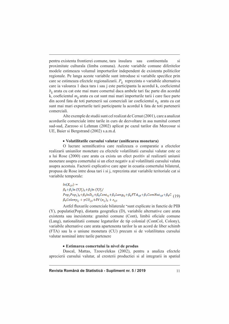
· Volatilitatile cursului valutar (unifi carea monetara) O lucrare semnifi cativa care realizeaza o comparatie a efectelor
realizarii uniunilor monetare cu efectele volatilitatii cursului valutar este ce
a lui Rose (2000) care arata ca exista un efect pozitiv al realizarii uniunii
monetare asupra comertului si un efect negativ a al volatilitatii cursului valuta
asupra acestuia. Factorii explicative care apar in ecuatia comertului bilateral,
propusa de Rose intre doua tari i si j, reprezinta atat variabile teritoriale cat si
variabile temporale:
(19)
Astfel fl uxurile comerciale bilaterale ־sunt explicate in functie de PIB (Y), populatie(Pop), distanta geografi ca (D), variabile alternative care arata
existenta sau inexistenta: granitei comune (Cont), limbii ofi ciale comune
(Lang), nationalitatii comune legaturilor de tip colonial (ComCol, Colony),
variabile alternative care arata apartenenta tarilor la un acord de liber schimb
(FTA) sau la o uniune monetara (CU) precum si de volatilitatea cursului
valutar nominal intre tarile partenere
· Estimarea comertului la nivel de produs Dascal, Mattas, Tzouvelekas (2002), pentru a analiza efectele
aprecierii cursului valutar, al cresterii productiei si al integrarii in spatiul
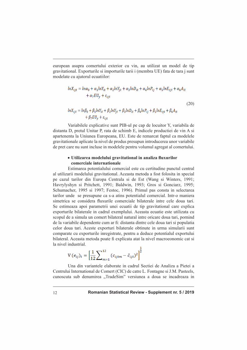
Romanian Statistical Review - Supplement nr. 5 / 201912
european asupra comertului exterior cu vin, au utilizat un model de tip
gravitational. Exporturile si importurile tarii i (membra UE) fata de tara j sunt
modelate cu ajutorul ecuatiilor:
(20)
Variabilele explicative sunt PIB-ul pe cap de locuitor Y, variabila de
distanta D, pretul Unitar P, rata de schimb E, indicele productiei de vin A si
apartenenta la Uniunea Europeana, EU. Este de remarcat faptul ca modelele
gravitationale aplicate la nivel de produs presupun introducerea unor variabile
de pret care nu sunt incluse in modelele pentru volumul agregat al comertului.
· Utilizarea modelului gravitational in analiza fl uxurilor
comerciale internationale
Estimarea potentialului comercial este cu certitudine punctul central
al utilizarii modelului gravitational. Aceasta metoda a fost folosita in special
pe cazul tarilor din Europa Centrala si de Est (Wang si Winters, 1991;
Havrylyshyn si Pritchett, 1991; Baldwin, 1993; Gros si Gonciarz, 1995;
Schumacher, 1995 si 1997; Festoc, 1996). Primul pas consta in selectarea
tarilor unde se presupune ca s-a atins potentialul comercial. Intr-o maniera
simetrica se considera fl uxurile comerciale bilaterale intre cele doua tari.
Se estimeaza apoi parametrii unei ecuatii de tip gravitational care explica
exporturile bilaterale in cadrul exemplului. Aceasta ecuatie este utilizata cu
scopul de a simula un comert bilateral natural intre oricare doua tari, pornind
de la variabile dependente cum ar fi : distanta dintre cele doua tari si populatia
celor doua tari. Aceste exporturi bilaterale obtinute in urma simularii sunt
comparate cu exporturile inregistrate, pentru a deduce potentialul exportului
bilateral. Aceasta metoda poate fi explicata atat la nivel macroeonomic cat si
la nivel industrial.
Una din variantele elaborate in cadrul Sectiei de Analiza a Pietei a
Centrului International de Comert (CIC) de catre L. Fontagne si J.M. Pasteels,
cunoscuta sub denumirea „TradeSim” versiunea a doua se incadreaza in
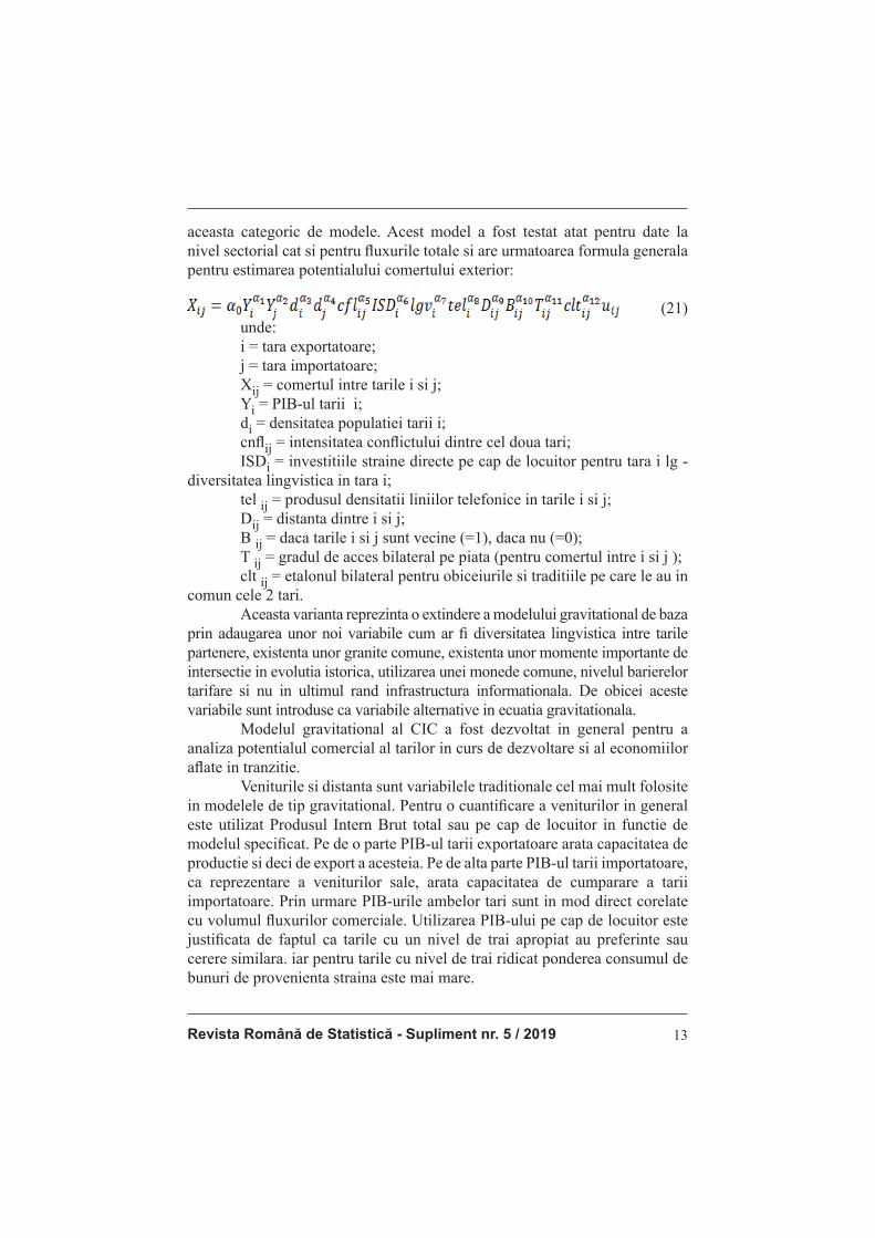
Revista Română de Statistică - Supliment nr. 5 / 2019 13
aceasta categoric de modele. Acest model a fost testat atat pentru date la
nivel sectorial cat si pentru fl uxurile totale si are urmatoarea formula generala
pentru estimarea potentialului comertului exterior:
(21)
unde:
i = tara exportatoare;
j = tara importatoare;
Xij = comertul intre tarile i si j;
Yi = PIB-ul tarii i;
di = densitatea populatiei tarii i;
cnfl ij = intensitatea confl ictului dintre cel doua tari;
ISDi = investitiile straine directe pe cap de locuitor pentru tara i lg -
diversitatea lingvistica in tara i;
tel ij = produsul densitatii liniilor telefonice in tarile i si j;
Dij = distanta dintre i si j;
B ij = daca tarile i si j sunt vecine (=1), daca nu (=0);
T ij = gradul de acces bilateral pe piata (pentru comertul intre i si j );
clt ij = etalonul bilateral pentru obiceiurile si traditiile pe care le au in
comun cele 2 tari.
Aceasta varianta reprezinta o extindere a modelului gravitational de baza
prin adaugarea unor noi variabile cum ar fi diversitatea lingvistica intre tarile
partenere, existenta unor granite comune, existenta unor momente importante de
intersectie in evolutia istorica, utilizarea unei monede comune, nivelul barierelor
tarifare si nu in ultimul rand infrastructura informationala. De obicei aceste
variabile sunt introduse ca variabile alternative in ecuatia gravitationala.
Modelul gravitational al CIC a fost dezvoltat in general pentru a
analiza potentialul comercial al tarilor in curs de dezvoltare si al economiilor
afl ate in tranzitie.
Veniturile si distanta sunt variabilele traditionale cel mai mult folosite
in modelele de tip gravitational. Pentru o cuantifi care a veniturilor in general
este utilizat Produsul Intern Brut total sau pe cap de locuitor in functie de
modelul specifi cat. Pe de o parte PIB-ul tarii exportatoare arata capacitatea de
productie si deci de export a acesteia. Pe de alta parte PIB-ul tarii importatoare,
ca reprezentare a veniturilor sale, arata capacitatea de cumparare a tarii
importatoare. Prin urmare PIB-urile ambelor tari sunt in mod direct corelate
cu volumul fl uxurilor comerciale. Utilizarea PIB-ului pe cap de locuitor este
justifi cata de faptul ca tarile cu un nivel de trai apropiat au preferinte sau
cerere similara. iar pentru tarile cu nivel de trai ridicat ponderea consumul de
bunuri de provenienta straina este mai mare.
Romanian Statistical Review - Supplement nr. 5 / 201914
In general sunt utilizate veniturile nominale transformate la rata de
schimb aferenta perioadei respective. Oricum, elasticitatea comertului functie
de venit poate fi alterata cand se iau in considerare economii in curs de dezvoltare
sau tari afl ate in tranzitie. Utilizarea PPP (Paritatii Puterii de Cumparare) poate de asemenea sa conduca la modifi cari a elasticitatii comertului in functie de
nivelul venitului. In cele din urma, s-a dovedit ca uneori PPP este mult mai
potrivita pentru a estima potentialul comercial pe termen lung, un orizont in
care evolutia ratei de schimb se apropie de echilibru. Pe termen scurt insa, este
mult mai potrivita utilizarea ratei de schimb nominale.
Un alt factor de infl uenta care, datorita importantei lui, a inceput sa apara frecvent in modelele de tip gravitational este gradul de accesibilitate al pietei. Deoarece modelul gravitational este prin constructie, in general, bilateral, este necesara o masura bilaterala a accesului pe piata care tine cont de toate regimurile preferentiale. 0 solutie este oferita de Bouet (2001) care propune un indicator care inglobeaza toate tipurile de taxe, tarife, contingente inclusiv masuri antidumping intr-o valoare unica. Aceste valori pentru fi ecare pereche de tari
partenere sunt cuprinse in baza de date MAC Map. Un tarif prea mare sau prea
mic, implica importuri prea mari, respectiv prea mici, iar contributia acestora la
protectia generala este redusa sau inregistreaza o crestere. Utilizand importurile
nationale ca ponderi se ajunge la o subevaluare a nivelului de protectie.
Pana la construirea bazei de date mai sus amintite au fost utilizate pe
scara larga variabile alternative pentru existenta acordurilor regionale. Pentru
ca in general tarile afl ate intr-un acord sunt in general si tari vecine sau tari cu un trecut istoric apropiat, exista riscul aparitiei multicoliniaritatii, situatie in care parametrii nu sunt unic determinati. Factorii culturali sunt deseori introdusi in modelul gravitational sub forma unor variabile alternative care, de regula, variaza, intre 0 si 1. Complexitatea aspectelor culturale este mult simplifi cata, in majoritatea
modelelor de tip gravitational, prin reducerea factorilor culturale la limba
nationala (fi e ofi ciala, fi e limba vorbita) si la legaturile de tip colonial. Date
extrem de utile pot fi preluate din „Exporters’ Ecncyclopedia” (Enciclopedia
Exportatorilor) editata de Dun & Bradstreet. De regula, in modelul gravitational traditional cheltuielile de tranzactionare si de transport sunt determinate de doua variabile: existenta unei granite comune si distanta fi zica intre cele doua tari. Asa cum se va putea
vedea in continuare, modele mai recente includ si alte variabile explicative
pentru cheltuielile de tranzactionare.
· Existenta granitelor comune este reprezentata in general de o
variabila alternativa care ia valoarea 1 in cazul in care tarile partenere sunt tari
vecine sau valoarea 0 in caz contrar.

Revista Română de Statistică - Supliment nr. 5 / 2019 15
Distanta este reprezentata de lungimea arcului de cerc dintre capitalele
sau principalele orase ale tarilor i si j. Latitudinea φ si longitudinea λ, celor
doua orase se transforma initial in radiani (II/360) iar apoi se calculeaza
distanta dupa urmatoarea formula:
(22)
unde:
z = 6367 (daca distanta este exprimata in km)
Loungani, Mody si Razin (2002) lanseaza ideea ca variabila
de distanta surprinde, pe langa cheltuielile propriu zise de transport, si
cheltuielile de informare si cercetare a pietei tarii de destinatie. Pentru a
surprinde in mod distinct efectul cheltuielilor de informare si cercetare autorii
au propus introducerea unei variabile care sa surprinda intensitatea structurii
informationale. Aceasta variabila se calculeaza ca produs al numarului de linii
telefonice pe cap de locuitor in cele doua tari partenere.
Un alt factor care infl uenteaza volumul comertului exterior este
calitatea infrastructurii de transport care poate fi apreciata prin procentajul
drumurilor pavate in lungimea totala a drumurilor sau ca densitate a lungimii
liniilor de cale ferata (lungime cale ferata raportata la suprafata). De obicei,
variabilele care exprima calitatea infrastructurii, fi e informationale fi e de
transport, sunt puternic corelate atat intre ele cat si cu PIB-ul pe cap de locuitor.
Prin urmare utilizarea lor in cadrul aceluiasi model ridica semne de intrebare.
Țarile mari au tendinta de a desfasura o buna pare a comertului pe
teritoriul tarii lor. Din aceasta cauza suprafata totala a unei tari poate fi folosita
pentru a explica volumul comertului directionat spre exterior.
Existenta Institutul de Cercetare a Confl ictelor Internationale din
Heidelberg deschide posibilitatea introducerii unei variabile de confl ict in
explicarea fl uxurilor comerciale. Conform defi nitiilor elaborate in cadrul
acestui institut exista patru forme majore care caracterizeaza intensitatea
confl ictelor internationale: confl ict latent, criza, criza severa si razboi carora
li se pot atribui valori de la 1 la 4 in ordinea cresterii intensitatii starii
confl ictuale. Variabila care se preteaza a fi introdusa intr-un model trebuie sa
fi e o combinatie intre intensitatea starii confl ictuale si durata ei.
Diversitatea lingvistica intr-o anumita tara este considerata un
stimul al comertului international. Indicele diversitatii lingvistice reprezinta
probabilitatea ca doua persoane alese la intamplare sa aiba limbi materne
diferite. Cu cat acest indice este mai apropiat de 1 cu atat este mai mare
diversitatea lingvistica in acea tara.

Romanian Statistical Review - Supplement nr. 5 / 201916
Gradul de pregatire intelectuala creeaza premise pentru comert, insa
este o variabila puternic corelata cu PIB-ul pe cap de locuitor si prin urmare
nu se recomanda introducerea celor doua variabile in acelasi model.
Fluxurile investitiilor straine directe pe cap de locuitor arata
atractivitatea de care se bucura o tara pe plan extern, arata gradul de
deschidere economica, stabilitatea mediului economic si legislativ, conduce
la dezvoltarea mediului tehnologic si a marketing-ului international. Toate
aceste premise si efecte ale ISD pot crea conditiile unui mediu prielnic pentru
dezvoltarea comertului exterior. Este necesara insa mentiunea ca impactul
ISD asupra exporturilor depinde si de natura investitiilor si de marimea tarii
gazda. Investitiile in tarile mari precum Rusia sunt directionate in primul rand
catre piata interna, spre deosebire de tari ca Estonia spre exemplu.
Pentru a crea o variabila explicative cat mai completa pentru fl uxurile
comerciale dintre doua tari partenere ar fi ideala utilizarea fl uxurilor de ISD
bilaterale dintre cele doua tari. Din pacate, fl uxurile bilaterale de ISD nu sunt
disponibile decat pentru tarile OCDE.
· Utilizarea modelului INTERLINK in generarea ecuatiilor comertului exterior
Modelul de echilibru global INTERLINK elaborat de OCDE este o
reprezentare a economiei mondiale si este format dintr-un set de submodele
pentru fi ecare tara membra OCDE impreuna cu ecuatiile de legaturi comerciale
si fi nanciare cu sase regiuni formate din tari non-membre OCDE. Prin cele peste
4000 de ecuatii pe care le contine, modelul INTERLINK trateaza economia
mondiala ca pe un tot integrat surprinzand aspecte multiple ale acesteia atat
din punctul de vedere al economiilor individuale cat si din punctul de vedere
al legaturilor internationale. Acest model, estimat pe date trimestriale, are un
rol operational in proiectiile si simularile pe care le realizeaza OCDE si care
sunt prezentate in publicatia „OECD Economic Outlook”.
Initial modelul INTERLINK a fost conceput ca un model al comertului
mondial care treptat s-a extins prin adaugarea unor relatii legate de cererea si
oferta agregate, salarii medii pe economie, preturile unor bunuri esentiale,
agregate monetare, rate ale dobanzii, cursuri de schimb valutar, situatii ale
bugetelor de stat si fl uxuri investitionale.
Relatiile de export, considerate in general ca fi ind in esenta
determinate de cerere, reprezinta comportamentul agentilor comerciali pe
o piata internationala care poseda un anumit grad de omogenitate si care
determina un comportament, intr-o anumita masura similar, al actorilor pe
piata internationala. Intr-un model al comertului international ne putem astepta
prin urmare ca parametrii care caracterizeaza comportamentul exportatorilor

Revista Română de Statistică - Supliment nr. 5 / 2019 17
pe o anumita piata sa prezinte un anumit grad de similitudine care poate sa
justifi ce abordarea comertului mondial printr-un sistem de ecuatii, impreuna
cu anumite restrictii care sa asigure consistenta comertului insumat al tarilor
individuale cu volumul cererii agregate la nivel mondial.
Setul ecuatiilor de export din cadrul modelului INTERLINK porneste,
ca de altfel multe alte modele din literature de specialitate, de la premisa unei
relatii inverse dintre performanta exportului si intensitatea competitivitatii pe
plan international. Performanta exportului unei tari este cuantifi cata ca si cota
de piata (volumul exportului raportat la cererea pietei de destinatie care la
randul ei este determinate ca o medie ponderata a importurile tarilor de pe
piata intenationala). Competitivitatea pe piata internationala este cuatifi cata
in termeni de preturi de export relative, preturile competitorilor din pietele
alternative fi ind ponderate si insumate.
Modifi carile competivitatii, cuantifi cate ca preturi relative, nu pot
sa explice evolutia performantei exporturilor in toata complexitatea ei. Prin
urmare, pe langa factorii de cerere (competitiviatatea mediului extern) este
utila introducerea unor elemente legate de calitatea produselor, de conditiile
de livrarea sau de distributie a acestora, adica a factorilor legati de oferta.
Aceste aspecte sunt insa mult mai greu de surprins intr-un model de natura
cantitativa. 0 alternativa, adoptata in cadrul INTERLINK, este modelarea
fl uctuatiilor care nu sunt explicate de competitivitatea preturilor, prin utilizarea unei functii de tendinta non-liniare. f (t) = exp(α(t – β)2) (23)
unde:
α < 0;
t = este variabila timp.
Decizia adoptarii unor astfel de functii a fost luata dupa ce in
prealabil a fost tatonata ideea utilizarii unor functii de tendinta liniare sau a
unor coefi cienti de elasticitate diferiti de unu care nu au putut insa surprinde
evolutia performantei exporturilor intr-un numar atat de divers de tari datorita
rigiditatii lor functionale. Functia nonliniara adoptata, prezentata anterior, are
o forma sufi cient de fl exibila si are proprietatea ca in timp tinde la 0 adica,
efectul ei asupra performantei exportului se anuleaza in timp.
Functia non-liniara are capacitatea de a surprinde modifi carile
performantei exporturilor care sunt legate de stadiul de dezvoltare al unei tari.
Schimbarile bruste de natura structurala, care implica trecerea de la exportul
de resurse primare la produse manufacturate iar apoi, intru-un stadiu mai
avansat la exportul de servicii sunt evidentiate intr-o prima faza de cresteri
exponentiale care se aplatizeaza pe masura maturizarii respectivei economii
nationale. Aceasta evolutia este insotita de fl uxurile de investitii straine directe
Romanian Statistical Review - Supplement nr. 5 / 201918
masive pentru aducerea mediului tehnologic dintr-o tara in curs de dezvoltare
la nivelul tarilor mai dezvoltate, din partea tarilor mai dezvoltate existand in
primul rand motivatia costurilor mai reduse ale fortei de munca. Noua teorie
a comertului care pune accentul pe importanta cresteri profi turilor bazate pe
economiile de scara si relatia dintre exporturi si rata de crestere a productiei
interne (Krugman 1989) justifi ca introducerea unor termeni legati de oferta
cum ar fi PIB-ul sau stocul de capital al tarii exportatoare. Functia de tendinta
non-liniara are rolul de a inlocui toti acesti factori si de a surprinde efectul
agregat al tuturor aspectelor legate de oferta.
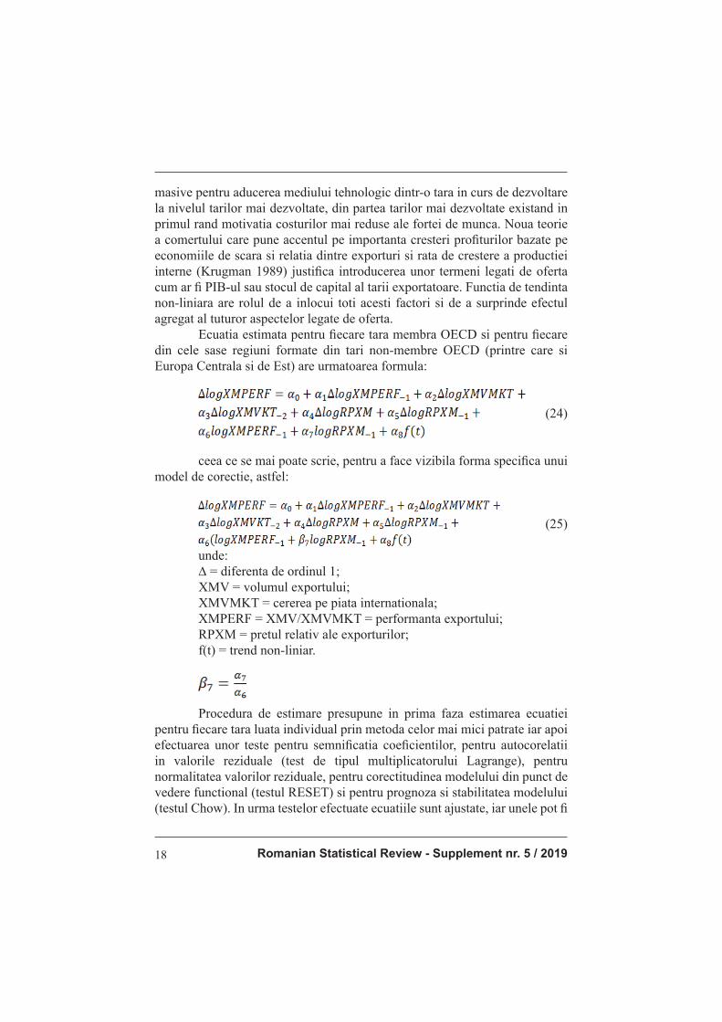
Ecuatia estimata pentru fi ecare tara membra OECD si pentru fi ecare
din cele sase regiuni formate din tari non-membre OECD (printre care si
Europa Centrala si de Est) are urmatoarea formula:
(24)
ceea ce se mai poate scrie, pentru a face vizibila forma specifi ca unui
model de corectie, astfel:
(25)
unde:
∆ = diferenta de ordinul 1;
XMV = volumul exportului;
XMVMKT = cererea pe piata internationala;
XMPERF = XMV/XMVMKT = performanta exportului;
RPXM = pretul relativ ale exporturilor;
f(t) = trend non-liniar.
Procedura de estimare presupune in prima faza estimarea ecuatiei
pentru fi ecare tara luata individual prin metoda celor mai mici patrate iar apoi
efectuarea unor teste pentru semnifi catia coefi cientilor, pentru autocorelatii
in valorile reziduale (test de tipul multiplicatorului Lagrange), pentru
normalitatea valorilor reziduale, pentru corectitudinea modelului din punct de
vedere functional (testul RESET) si pentru prognoza si stabilitatea modelului
(testul Chow). In urma testelor efectuate ecuatiile sunt ajustate, iar unele pot fi
Revista Română de Statistică - Supliment nr. 5 / 2019 19
chiar eliminate. Se trece apoi la abordarea setului de ecuatii ca sistem, ecuatiile
avand coefi cienti comuni, fi xati in plan teritorial pentru toate variabilele mai
putin pentru functia de tendinta f(t). Datorita faptului ca in urma estimarii
sistemului cu ajutorul metodei celor mai mici patrate s-a obtinut o corelatie
semnifi cativa intre valorile reziduale in plan teritorial, adica intre valorile
reziduale corespunzatoare diverselor tari, s-a hotarat adoptarea metodei de
estimare SURE (Seemingly Unrelated Regression Estimation). Merita amintit
faptul ca tari recent integrate in UE care sunt si membre OECD (Ungaria,
Cehia, Polonia) ridica probleme in procesul de estimare datorita numarului
redus de date.
Romania nefi ind membra OCDE nu este surprinsa in setul de ecuatii
pentru comertul exterior din cadrul modelului INTERLINK ca tara individuala
ci doar membra a unei grupe de tari non-membre. Propuneri specifi ce pentru
modelarea comertului Romaniei, atat sub forma unor modele de corectie, cat
si sub alte forme, sunt facute in capitolul patru. Lipsa unui numar sufi cient de
date statistice va reprezenta si acest caz insa un obstacol in calea obtinerii unor
rezultate cu o semnifi catie statistica ridicata.
Conclusions O serie de elemente sunt preluate din studiile efectuate de mulți
cercetători, astfel încât modelul gravitațional a ajuns din punct de vedere
teoretic un model utilizabil în studiile comerțului internațional.. Așa depildă
se explică variabila dependentă, de natura comerțului internațional prin
combinarea unor variabile macro-economice. rezultă că ecuația gravitațională
poate fi utilizată cu succes pentru a estima atât factorii de volum cât și factorii
privind natura fl uxurilor comerciale. Teoria privind utilizarea acestui model
este bazată pe indicatori cu grad redus de complexitate pentru care există
valori înregistrate în majoritatea țarilor pe o perioadă sufi cient de lungă.
Apreciem că modelul gravitațional, prin natura variabilelor independente,
se pretează la analiza comețului internațional la un nivel ridicat de agregare.
Acest model poate fi utilizat și în analiza structurală a comețului internațional
pe categorii de produse sau chiar pe produse și servicii considerate. Autorii
evidențiază relațiile matematice utilizabile în cazul analizelor pe baza
modelului gravitațional.
References 1. Anghelache, C., Anghel, M.G. (2018). Econometrie generală. Teorie și studii de
caz, Editura Economică, Bucureşti
2. Anghelache, C., Anghel, M.G. (2016). Bazele statisticii economice. Concepte
teoretice şi studii de caz, Editura Economică, Bucureşti
Romanian Statistical Review - Supplement nr. 5 / 201920
3. Anghelache, C., Mitruţ, C., Voineagu, V. (2013). Statistică macroeconomică. Sistemul Conturilor Naţionale, Editura Economică, Bucureşti
4. Anghelache, C., Pârţachi, I., Gonţa E., Kralik, L. (2012). Gravitational Model for the Analysis of Commercial Flows, International Conference “Conjuncture and quality trends in the economic development of society”, April 26-28, 2012, Romanian Statistical Review, Supplement, 261-268
5. Anghelache, C. (2008). Tratat de statistică teoretică şi economică, Editura Economică, Bucureşti
6. Arcidiacono, P., Miller, R.A. (2011). Conditional Choice Probability Estimation of Dynamic Discrete Choice Models with Unobserved Heterogeneity. Econometrica, 79 (November 2011), 1823-1867
7. Benjamin, C., Herrard A., Hanee-Bigot, M., Tavere, C. (2010). Forecasting with
an Econometric Model, Springer 8. Corbare, D., Durlauf, S., Hansen, B. (2006). Econometric Theory and Practice
- Frontiers of Analysis and Applied Research, Cambridge University Press 9. Dascal, M., Mattas, K., Tzouvelekas, V. (2002). An analysis of EU wine trade:
A gravity model approach. International Advances in Economic Research, 8 (2), 135-147
10. Elliott, G., Müller, U.K., Watson, M.W. (2015). Nearly Optimal Tests When a Nuisance Parameter is Present Under the Null Hypothesis. Econometrica, 83, 771-811
11. Johansen, S., Nielsen, M. (2010). Likelihood inference for a fractionally
cointegrated vector autoregressive model, CREATES Research Papers 2010-24, School of Economics and Management, University of Aarhus
12. Müller, U.K. (2007). A Theory of Robust Long-Run Variance Estimation. Journal
of Econometrics, 141, 1331-1352. 13. Newbold, P., Karlson, L.W., Thorne, B. (2010). Statistics for Business and
Economics, 7th ed., Pearson Global Edition, Columbia, U.S 14. Pesavento, E., Rossi, B. (2006). Small–sample Confi dence Interevals for
Multivariate Impulse Response Functions at Long Horizons. Journal of Applied
Econometrics, 21 (8), 1135–1155 15. Phillips, P.C.B., Sun, Y., Jin, S. (2006). Spectral Density Estimation and Robust
Hypothesis Testing using Steep Origin Kernels without Truncation. International
Economic Review, 47, 837-894.

Revista Română de Statistică - Supliment nr. 5 / 2019 21
THE GRAVITATIONAL MODEL USED IN THE ECONOMIC ANALYZES
Prof. Constantin ANGHELACHE PhD ([email protected])
Bucharest University of Economic Studies / „Artifex” University of Bucharest
Prof. Gabriela Victoria ANGHELACHE PhD ([email protected])
Bucharest University of Economic Studies
Assoc. Mădălina-Gabriela ANGHEL PhD ([email protected])
„Artifex” University of Bucharest
Gabriel-Ștefan DUMBRAVĂ PhD Student ([email protected])
Bucharest University of Economic Studies
Oana-Ana-Maria SIMA Master Student
Abstract Numerous empirical studies have shown that trade fl ows follow the
principles of gravity-related physics: two opposing forces determine the
level of bilateral trade between countries, the level of economic activity
and income, on the one hand, and all the barriers to trade, on the other.
The latter include: transport costs, prohibitive trade policies, insecurity of
exporters and importers about the evolution of various trade conditions such
as the evolution of the exchange rate, cultural diff erences, the existence of
national borders, the diversity of consumer preferences and various other
impediments. The authors’ analysis highlights the fact that the gravitational
model ensures the possibility of international trade analysis. Gravitational
equations have several characteristics that make it possible to carry out
empirical studies being a bilateral equation. Although the gravitational
model had, since the beginning of its use, an empirical success that could
be challenged with diffi culty, this model had, however, for some time, also
criticism regarding the lack of a theoretical substantiation. From that moment
on, it has been increasingly accepted that the gravitational equation can be
extracted from certain hypotheses from theoretical models such as ricardian
models, Heckscher-Ohlin models or scale models belonging to New Theories
of International Trade. These three types of models diff er in essence by the
way in which product specialization is made by diff erent countries.
Keywords: international trade, regionalization, import, export,
exchange rate, gravity model, interlink model.
JEL Classifi cation: C50, F13, F40
Romanian Statistical Review - Supplement nr. 5 / 201922
Introduction The equation of gravity is one of the most used tools in empirical
studies on international trade issues. Although the main objective of the
gravitational model is the estimation of the commercial potential, other
directions of use of this model can be mentioned, such as: the estimation of
the costs that the frontiers between nations involve, the explanation of the
cyclical evolution of the international trade, the identifi cation of the eff ects
of the regionalization, and last but not least explaining the eff ect of various
economic variables on trade such as for example the impact of volatility or
the evolution of currency exchange on commerce and so on The number of
explanatory variables and the variety of forms in which they are quantifi ed have
experienced such an explosion over the past 20 years that a mere enumeration
of them becomes rather diffi cult and risks being incomplete. Therefore,
there is a presentation of the most important uses of the gravitational model
along with the most signifi cant variables without having the requirement of a
complete presentation..
Literature review Anghelache and Anghel (2018) and Corbare, Durlauf and Hansen
(2006) analyzed the main econometric methods and models used in economic
analyzes. Anghelache (2008) presented the statistical indicators applied in the
study of international trade. A similar theme is analyzed by Anghelache and
Anghel (2016). Anghelache, Mitruţ and Voineagu (2013) studied fundamental
aspects of macroeconomic statistics. AnghelachePârţachi, Gonţa and Kralik
(2012) analyzed elements related to the gravitational model. Arcidiacono
and Miller (2011) investigated concepts of dynamic models. Benjamin,
Herrard, Hanee-Bigot and Tavere (2010) analyzed the use of econometric
models in predictive activity. Dascal, Mattas, and Tzouvelekas (2002) used
a gravitational model to study the infl uence of exchange rate fl uctuations on
foreign trade. Elliott, Müller and Watson (2015), and Phillips, Sun and Jin
(2006) studied aspects of econometric models testing. Johansen and Nielsen
(2010) referred to inference in autoregressive models. Müller (2007) studied
the estimation of long-term variations. Newbold, Karlson and Thorne (2010)
analyzed basic elements of economic statistics. Pesavento and Rossi (2006)
analyzed aspects of sampling.
Methodology, data, results and discussions The gravitational model for international trade fl ows originates in the
law of universal attraction proposed by Newton (1687) which makes known
and unanimously accepted that the force of attraction between two bodies

Revista Română de Statistică - Supliment nr. 5 / 2019 23
i and j is directly proportional to the product of the masses and inversely
proportional to the square of the distances:
(1)
Mj = mass of the two bodies;
Dij = distance between the two bodies;
G = gravitational constant.
The similarity is striking with the gravitational model in its traditional
version, as it is presented in „Deardorff Glossary of International Economics”
with the following equation for estimating exports:
Tij = AYi Yj /Dij (2)
where:
Tij = export from country to country j;
A = constant;
Yi ,Yj = national income;
Dij = distance between the two countries.
This model, originally having an economic theory of origin, and
representing more of a universal law taken from physics, is also attributed
to Jan Tinbergen (1962) and Pentti Poyhonen (1963). The model was also
taken up by other social sciences and used to simulate tourist fl ows, migratory
fl ows between diff erent countries, buyers fl ows to diff erent shopping malls
s.a.m.d. assuming of course that these phenomena are based on the same law
of universal attraction.
Although it is diffi cult to fi nd a common denominator of all specialized
papers that have been elaborated in this fi eld, however, the most common
variant of the gravitational model could be represented by the following
equation:
(3)
where: Xij = total exports from i to j;
Yi ,Yj = country revenue;
Li,Lj = population;
Dij = geographic distance between i and j;
Pij = degree of market access from i to j;
Uij = normal and identically distributed random variable, i.i.d. N(0,
)
The formula can be written as follows:
(4)
where: yi and yj = income per capita of the partner countries so
Romanian Statistical Review - Supplement nr. 5 / 201924
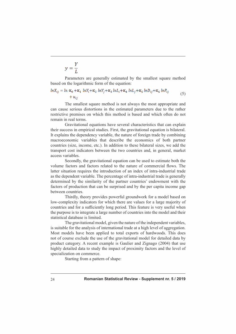
Parameters are generally estimated by the smallest square method
based on the logarithmic form of the equation:
(5)
The smallest square method is not always the most appropriate and
can cause serious distortions in the estimated parameters due to the rather
restrictive premises on which this method is based and which often do not
remain in real terms.
Gravitational equations have several characteristics that can explain
their success in empirical studies. First, the gravitational equation is bilateral.
It explains the dependency variable, the nature of foreign trade by combining
macroeconomic variables that describe the economics of both partner
countries (size, income, etc.). In addition to these bilateral sizes, we add the
transport cost indicators between the two countries and, in general, market
access variables.
Secondly, the gravitational equation can be used to estimate both the
volume factors and factors related to the nature of commercial fl ows. The
latter situation requires the introduction of an index of intra-industrial trade
as the dependent variable. The percentage of intra-industrial trade is generally
determined by the similarity of the partner countries’ endowment with the
factors of production that can be surprised and by the per capita income gap
between countries.
Thirdly, theory provides powerful groundwork for a model based on
low-complexity indicators for which there are values for a large majority of
countries and for a suffi ciently long period. This feature is very useful when
the purpose is to integrate a large number of countries into the model and their
statistical database is limited.
The gravitational model, given the nature of the independent variables,
is suitable for the analysis of international trade at a high level of aggregation.
Most models have been applied to total exports of hardwoods. This does
not of course exclude the use of the gravitational model for detailed data by
product category. A recent example is Gaulier and Zignago (2004) that use
highly detailed data to study the impact of proximity factors and the level of
specialization on commerce.
Starting from a pattern of shape:

Revista Română de Statistică - Supliment nr. 5 / 2019 25
(6)
where:
α = constant in time and space;
αt = fi xed eff ect, specifi c for each period t and constant in the territorial
plane;
αij = fi xed eff ect, specifi c to each pair ij and constant over time;
PIBEit, PIBIjt = GDP per capita of the respective exporter and importer;
PEi,,PIjt, = the exporter / importer’s population;
Dij = distance between the two countries;
εij = the random and identically distributed random variable of mean
1 and constant variation, i. i.d. (1,σ ) which by logarithm will become:
(7)
we can interpret parameter β as the elasticity of export by infl uence
factors after the following reasoning.
By fi rst degree diff erentiation after the temporal variable t, the
equation above becomes
(8)
It is known that the logarithm diff erence approximates the rhythm of
growth:
(9)
the approximation being stronger as the diff erence from period t-1 to
period t is lower.
Consequently, the coeffi cients βi i=1,4 show the change in the
growth rate of exports at the change by 1 (100% in percentage expression) of
the growth rate in the evolution of the infl uence factors.
In order to obtain the interpretation of the β5, coeffi cient, corresponding
to a purely territorial variable, proceed analogously, but this time the fi rst
order diff erences will be made on a territorial level. We assume that pairs of
countries ij are ordered according to a certain criterion. The diff erences of the
consecutive pairs for a fi xed year would not look like this:
Romanian Statistical Review - Supplement nr. 5 / 201926
(10)
The coeffi cient β5 will now have the same interpretation as the other
coeffi cients, with the diff erence with the variance being manifested in the
territorial and not temporal plan.
Equation (6) can not be estimated directly due to the collinearity
between territorial variables of distance, Dij specifi es each pair of countries
and the constant over time and the fi xed eff ect, specifi c to each αij pair, both
having the same properties and the same territorial variation. Therefore we
will alternately remove the two variables..
• Model of the analysis of the international trade structure Trade overlaps (import and export to the same industry) are examined
by Bergstrand (1989) and Hummels and Levinsohn (1995). They have
constructed bilateral trade indices at industrial level in terms of intra-industry
trade. These indicators are aggregated nationwide and their weighted average
is explained using a gravitational equation. An alternative method used to
diff erentiate inter-industrial trade from intra-industrial trade fl ows is explained
in Fontagne, Freudenberg and Peridy (1998). In the above-mentioned works
we estimate the weights in the total trade of the types of trade, diff erentiating
in this way the vast majority of the gravitational models that generally estimate
the total volume of external sales.
Two recent works on this line are Kandogan (2004) and (2004). In
the last paper it is shown that the explanatory variables have diff erent eff ects
on diff erent components of the foreign trade and that as the economies of the
two countries and the supply of production factors become more and more
similar, the volume of horizontal intra-industrial trade increases. In the model
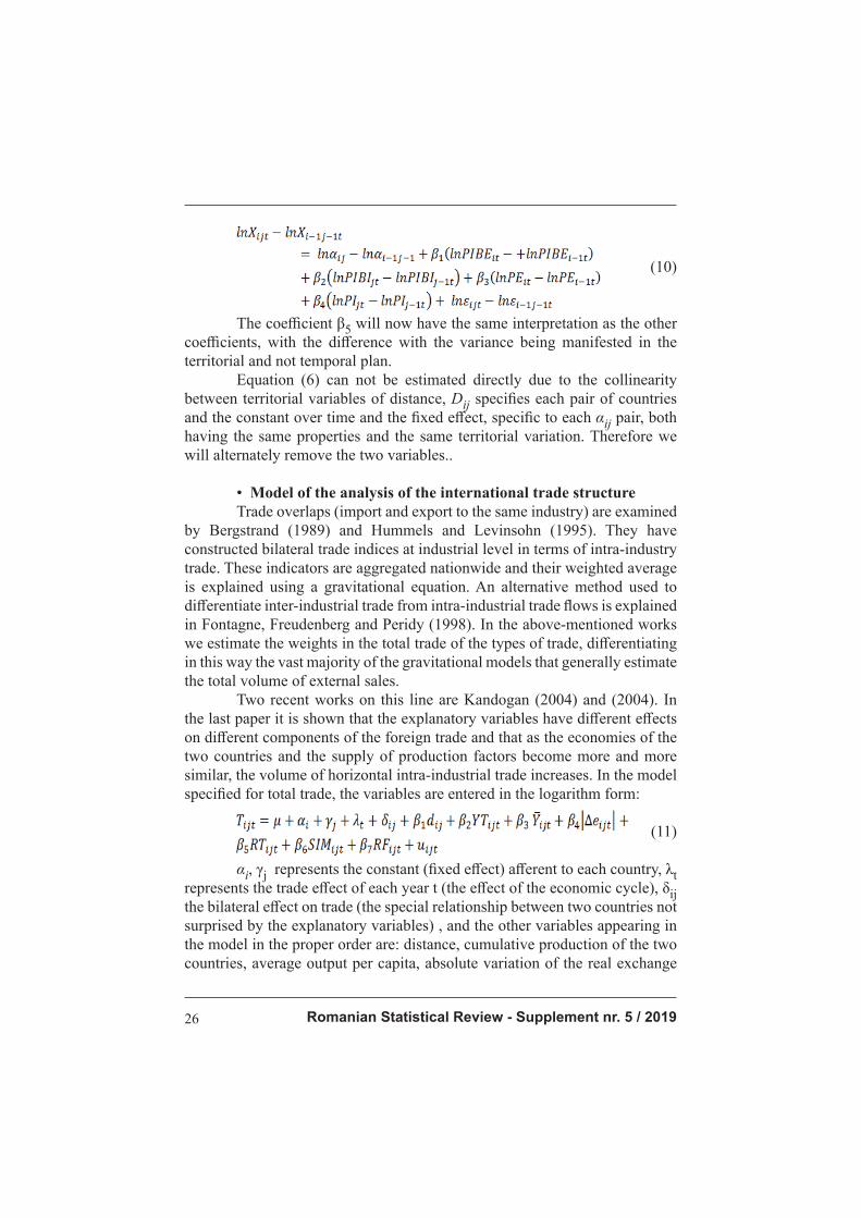
specifi ed for total trade, the variables are entered in the logarithm form:
(11)
αi, γj represents the constant (fi xed eff ect) aff erent to each country, λt
represents the trade eff ect of each year t (the eff ect of the economic cycle), δij the bilateral eff ect on trade (the special relationship between two countries not
surprised by the explanatory variables) , and the other variables appearing in
the model in the proper order are: distance, cumulative production of the two
countries, average output per capita, absolute variation of the real exchange

Revista Română de Statistică - Supliment nr. 5 / 2019 27
rate, total foreign exchange reserve, country similarity and diff erence in
endowment with factors of production. The last two variables will be detailed
in the following because they are not directly observable from offi cial statistics.
The SIM variable takes the value ln (0.5) when the cloudy ones get identical
production, high degree of similarity and decrease when the diff erence
between countries increases:
(12)
The diff erence in production factor, RF, is calculated according to the
capital stock K and the labor force L of the partner countries i and j at time t
following the following formula:
(13)
The capital stock, K, can be obtained by means of gross fi xed capital
formation. This indicator takes the value 0 when countries have the same
production factor endowment rate and increase with increasing country
diff erences.
The same type of model was then applied to import components to
capture how causal variables exert infl uence on the components. Internal trade components were identifi ed as intra-industry trade, vertical and horizontal, as
well as inter-industry trade. Intra-industry trade is calculated by formula:
(14)
where:
Mkijt = importing country i from country j into industry k.
The formula for inter-industry trade is:
(15)
The horizontal intra-industry imports can be defi ned as intra-Austrian
imports with the same product type p:
(16)
where:
Mkpijt = represents imports in country and country j for product p in
industry k at time t.

Romanian Statistical Review - Supplement nr. 5 / 201928
Imports of vertical intra-industry, ie trade in the same industry but with diff erent
products or products of diff erent processing grades, are thus calculated:
(17)
• Estimating the eff ects of regionalization in international trade The gravitational models have been widely used to assess the
infl uence of commercial policy measures on trade fl ows and, in particular, the
infl uence of regional integration agreements. If we consider the example of
the two countries between which a regional integration agreement has been
concluded, an alternative variable that takes the value 1 may be introduced if
the two countries are at a time t in the bilateral agreement and 0 otherwise. If
the estimated parameter of the alternative variable is positive and signifi cant
then it can be concluded that regionalization creates trade fl ows. This estimate
can be made in order to simulate the commercial potential corresponding to
any regional integration between diff erent groups of countries.
An example of a model for which the most important regional
agreements are considered, including the European Union, is that used by
Soloaga and Winters (2001). The model used also takes into consideration
traditional and variable variables such as those mentioned above. The equation
empirically tested on the imports of 58 countries during 1980-1996 is:
(18)
The value of country and country imports is explained by GDP,
population, two distance variables, country surface, alternative variables for
the existence of the common border, insular or continental country and cultural
proximity (common language). These variables common to diff erent models
estimate the volume of imports independent of the existence of regional
policies. In addition to these variables, specifi c variables are introduced to
estimate the eff ects of regionalization. Pk is an alternative variable that takes
the value 1 if country i or j is a participant to the k agreement, the bk coeffi cient
shows the higher the trade if both countries are part of the k agreement, the mk
coeffi cient shows the higher the country’s imports and is part of the agreement
against all its trading partners and the nk coeffi cient shows the higher the
exports of the country participating in the agreement k to all trading partners.

Revista Română de Statistică - Supliment nr. 5 / 2019 29
Other examples of studies are those conducted by Cernat (2001),
which analyzed trade agreements between developing countries in so-called
south-south trade Zarzoso and Lehman (2002) applied to the Mercosur and
EU countries, Baier and Bergstrand (2002) et al.
• Exchange rate volatility (monetary unifi cation) A signifi cant work that compares the eff ects of monetary union with
the eff ects of exchange rate volatility is that of Rose (2000), which shows that
there is a positive eff ect of monetary union on trade and a negative eff ect of
exchange rate volatility on it. The explanatory factors appearing in the bilateral
trade equation proposed by Rose between two countries i and j represent both
territorial variables and temporal variables:
(19)
Thus, bilateral trade fl ows - are explained by GDP (Y), population
(Pop), geographical distance (D), alternative variables that show existence or
nonexistence: common border (Cont), common language (ComCol, Colony),
alternative variables that show countries belonging to a Free Trade Agreement
(FTA) or a monetary union (CU) and the volatility of the nominal exchange
rate between partner countries
• Estimation of commerce at product level Dascal, Mattas, Tzouvelekas (2002) used a gravitational model to
analyze the eff ects of foreign exchange appreciation, production growth and
integration in European space on wine trade. Exports and imports of country i
(EU member) to country j are modeled using equations:
(20)
The explanatory variables are GDP per capita Y, D variable, Unitary
P, E exchange rate, A wine production index and EU membership, EU. It
is noteworthy that gravity models applied at the product level involve the

Romanian Statistical Review - Supplement nr. 5 / 201930
introduction of price variables that are not included in the models for the
aggregate volume of trade.
• Using the gravitational model in the analysis of international
trade fl ows
Estimating the commercial potential is certainly the central point of
using the gravitational model. (Wang and Winters, 1991; Havrylyshyn and
Pritchett, 1991; Baldwin, 1993; Gros and Gonciarz, 1995; Schumacher, 1995
and 1997; Festoc, 1996). The fi rst step is to select countries where trade
potential is presumed to have been achieved. In a symmetrical manner, bilateral
trade fl ows between the two countries are considered. We then estimate the
parameters of a gravitational equation that explains bilateral exports in the
example. This equation is used to simulate a natural bilateral trade between
any two countries, starting from dependent variables such as the distance
between the two countries and the population of the two countries. These
bilateral exports resulting from simulation are compared to registered exports
to deduce bilateral export potential. This method can be explained at both
macroeconomic and industrial level.
One of the variants developed by the International Trade Center
(CIC) Market Review Section by L. Fontagne and J.M. Pasteels, known as the
„TradeSim” second version fall into this categorical pattern. This model has
been tested for both sectoral and total data fl ows and has the following general
formula for estimating the potential for external trade:
(21)
where:
i = exporting country;
j = importing country;
Xij = trade between countries i and j;
Yi = GDP of the country i;
di = population density of the country i;
cnfl ij = the intensity of the confl ict between the two countries;
ISDi = foreign direct investment per capita for the country i;
lg = linguistic diversity in the country i;
tel ij = product density of telephone lines in countries i and j;
Dij = distance between i and j;
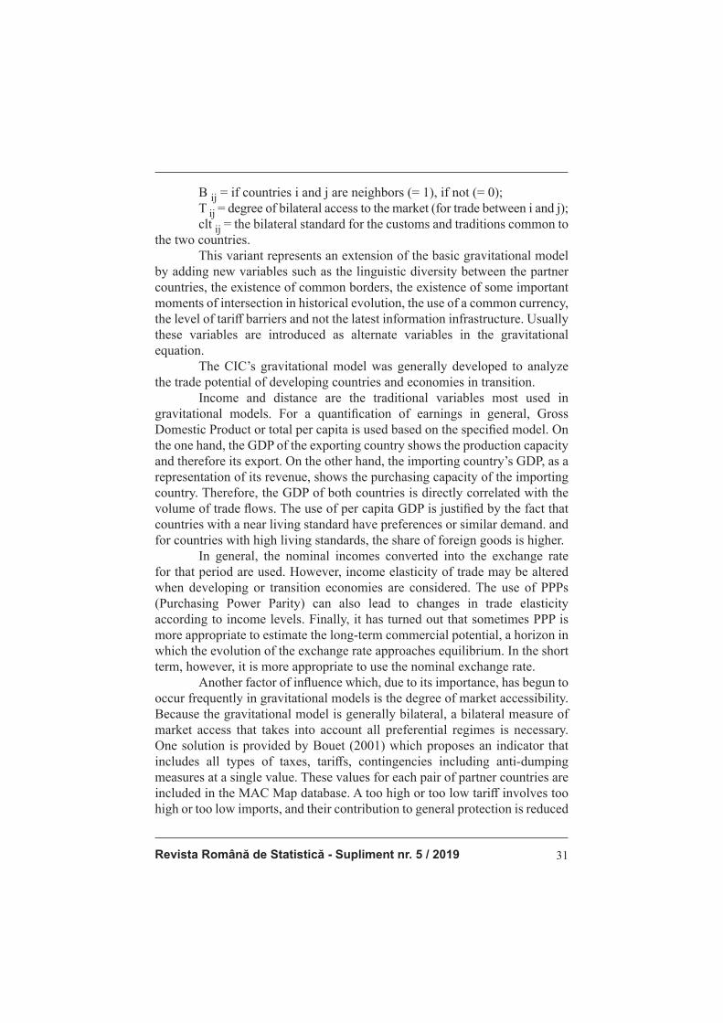
Revista Română de Statistică - Supliment nr. 5 / 2019 31
B ij = if countries i and j are neighbors (= 1), if not (= 0);
T ij = degree of bilateral access to the market (for trade between i and j);
clt ij = the bilateral standard for the customs and traditions common to
the two countries.
This variant represents an extension of the basic gravitational model
by adding new variables such as the linguistic diversity between the partner
countries, the existence of common borders, the existence of some important
moments of intersection in historical evolution, the use of a common currency,
the level of tariff barriers and not the latest information infrastructure. Usually
these variables are introduced as alternate variables in the gravitational
equation.
The CIC’s gravitational model was generally developed to analyze
the trade potential of developing countries and economies in transition.
Income and distance are the traditional variables most used in
gravitational models. For a quantifi cation of earnings in general, Gross
Domestic Product or total per capita is used based on the specifi ed model. On
the one hand, the GDP of the exporting country shows the production capacity
and therefore its export. On the other hand, the importing country’s GDP, as a
representation of its revenue, shows the purchasing capacity of the importing
country. Therefore, the GDP of both countries is directly correlated with the
volume of trade fl ows. The use of per capita GDP is justifi ed by the fact that countries with a near living standard have preferences or similar demand. and for countries with high living standards, the share of foreign goods is higher. In general, the nominal incomes converted into the exchange rate for that period are used. However, income elasticity of trade may be altered when developing or transition economies are considered. The use of PPPs (Purchasing Power Parity) can also lead to changes in trade elasticity according to income levels. Finally, it has turned out that sometimes PPP is more appropriate to estimate the long-term commercial potential, a horizon in which the evolution of the exchange rate approaches equilibrium. In the short term, however, it is more appropriate to use the nominal exchange rate. Another factor of infl uence which, due to its importance, has begun to occur frequently in gravitational models is the degree of market accessibility. Because the gravitational model is generally bilateral, a bilateral measure of market access that takes into account all preferential regimes is necessary. One solution is provided by Bouet (2001) which proposes an indicator that includes all types of taxes, tariff s, contingencies including anti-dumping
measures at a single value. These values for each pair of partner countries are
included in the MAC Map database. A too high or too low tariff involves too
high or too low imports, and their contribution to general protection is reduced
Romanian Statistical Review - Supplement nr. 5 / 201932
or increases. Using national imports as weights leads to an underestimation of
the level of protection.
Until the construction of the abovementioned database, there have
been widely used alternative variables for the existence of regional agreements.
Because in general the countries in an agreement are generally neighbors or
countries with a close historical past, there is a risk of multicollinearity, where
the parameters are not uniquely determined.
Cultural factors are often introduced into the gravitational model in the
form of alternative variables that typically range between 0 and 1. The complexity
of cultural aspects is much simplifi ed in most gravitational models by reducing
cultural factors to the national language (either offi cial, or spoken language)
and colonial ties. Extremely useful data can be downloaded from „Exporters’
Ecccyclopedia” (Encyclopedia of Exporters) edited by Dun & Bradstreet.
Typically, in the traditional gravitation model, transaction and
transportation costs are determined by two variables: the existence of a
common border and the physical distance between the two countries. As will
be seen later, more recent models include other explanatory variables for
transaction costs.
• The existence of common borders is generally represented by
an alternative variable that takes the value 1 if the partner countries are
neighboring countries or the value 0 otherwise.
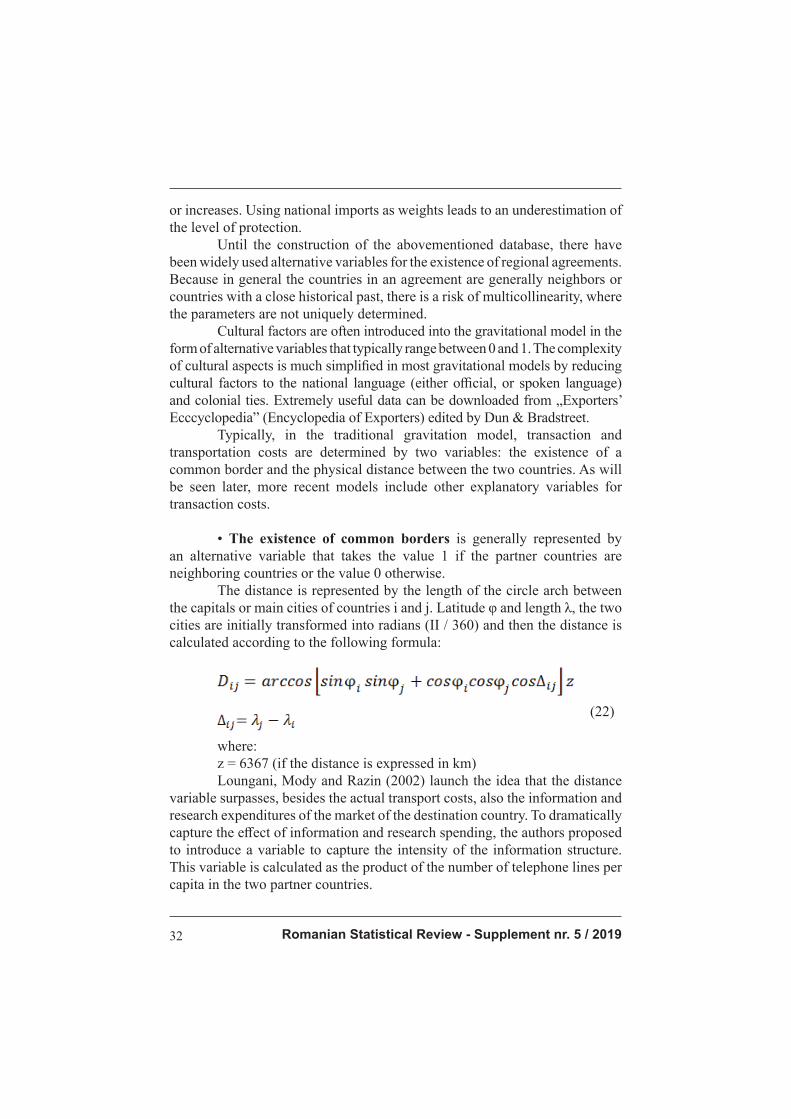
The distance is represented by the length of the circle arch between
the capitals or main cities of countries i and j. Latitude φ and length λ, the two
cities are initially transformed into radians (II / 360) and then the distance is
calculated according to the following formula:
(22)
where:
z = 6367 (if the distance is expressed in km)
Loungani, Mody and Razin (2002) launch the idea that the distance
variable surpasses, besides the actual transport costs, also the information and
research expenditures of the market of the destination country. To dramatically
capture the eff ect of information and research spending, the authors proposed
to introduce a variable to capture the intensity of the information structure.
This variable is calculated as the product of the number of telephone lines per
capita in the two partner countries.
Revista Română de Statistică - Supliment nr. 5 / 2019 33
Another factor infl uencing the volume of external trade is the quality
of the transport infrastructure, which can be appreciated by the percentage of
paved roads in the total length of the roads or as the density of the length of the
railway tracks (surface length of the railroad). Typically, variables that express
the quality of the infrastructure, either information or transport, are strongly
correlated with each other and with GDP per capita. Therefore, using them
within the same model raises questions.
Large countries tend to develop a good trade in their country. This is
why the total surface of a country can be used to explain the volume of trade
directed towards the outside.
The existence of the Heidelberg International Confl ict Research
Institute opens the possibility of introducing a confl ict of interest in explaining
trade fl ows. According to the defi nitions developed within this institute, there
are four major forms that characterize the intensity of international confl icts:
latent confl ict, crisis, severe crisis and war, which can be assigned values from
1 to 4 in order of increasing the intensity of the confl ict state. The variable that
is likely to be introduced into a model must be a combination of the intensity
of the confl ict state and its duration.
Linguistic diversity in a particular country is considered a stimulus of
international trade. The index of linguistic diversity is the likelihood that two
people randomly chosen will have diff erent mother tongues. The closer this
index is to 1, the linguistic diversity in that country is greater.
The degree of intellectual training creates prerequisites for commerce,
but it is a strongly correlated variable with per capita GDP and therefore it is
not recommended to introduce the two variables into the same model.
FDI fl ows per capita show the attractiveness a country enjoys
externally, shows the degree of economic openness, the stability of the
economic and legislative environment, leads to the development of the
technological environment and international marketing. All these premises
and eff ects of FDI can create the conditions for a favorable environment for
the development of foreign trade. It is necessary, however, to mention that the
impact of FDI on exports depends on the nature of the investments and on
the size of the host country. Investments in large countries such as Russia are
primarily directed towards the domestic market, unlike countries like Estonia
for example.
To create the most comprehensive explanatory variable for trade
fl ows between two partner countries, it would be ideal to use bilateral FDI
fl ows between the two countries. Unfortunately, bilateral FDI fl ows are only
available for OECD countries.

Romanian Statistical Review - Supplement nr. 5 / 201934
• Using the INTERLINK model in generating the foreign trade equations
INTERLINK global equilibrium model developed by the OECD is a
representation of the world economy and is composed of a set of sub-models
for each OECD member country with trade and fi nancial equations with six
regions consist of non-OECD countries. With its over 4,000 equations, the
INTERLINK model treats the world economy as an integrated one, capturing
multiple aspects of it, both in terms of individual economies and in terms of
international ties. This model, estimated on quarterly data, has an operational
role in the OECD projections and simulations that are presented in the OECD
Economic Outlook.
Originally, the INTERLINK model was designed as a model of
world trade that gradually expanded by adding aggregate supply and demand,
average salary to economy, key commodity prices, monetary aggregates,
interest rates, exchange rates, of state budgets and investment fl ows.
Export relations, generally considered to be essentially demand-
driven, represent the behavior of commercial agents on an international
market that possesses a certain degree of homogeneity and which leads
to somewhat similar behavior of actors on the international market. In a
pattern of international trade, we can therefore expect that the parameters
that characterize exporters’ behavior on a certain market will show a certain
degree of similarity that can justify approaching world trade through a system
of equations, along with certain restrictions to ensure the consistency of the
aggregate trade of individual countries with aggregate aggregate demand in
the world.
The set of export equivalences in the INTERLINK model, like
many other specialty literature models, starts from the premise of an inverse
relationship between export performance and international competitiveness.
The export performance of a country is quantifi ed as the market share (the
volume of export compared to the demand of the destination market, which
in turn is determined as a weighted average of the countries’ imports from the
intentional market). Competitiveness on the international market is quoted in
terms of relative export prices, with the prices of competitors in the alternative
markets being weighted and summed up.
Changes in competitiveness, quantifi ed as relative prices, can not
explain the evolution of export performance in all its complexity. Therefore,
besides the demand factors (competitiveness of the external environment),
it is useful to introduce elements related to the quality of the products,
their delivery or distribution conditions, ie the factors related to the supply.
These aspects are much more diffi cult to capture in a quantitative nature. An

Revista Română de Statistică - Supliment nr. 5 / 2019 35
alternative, adopted within INTERLINK, is the modeling of fl uctuations that
are not explained by price competitiveness through the use of a non-linear
trend function.
f (t) = exp(α(t – β)2) (23)
where:
α < 0;
t = is the variable time.
The decision to adopt such functions was taken after the idea of
using linear trending functions or coeffi cients of elasticity diff erent from one
that could not surprising the evolution of export performance in such a large
number of countries due to their functional rigidity. The nonlinear adopted
feature, previously presented, has a suffi ciently fl exible form and has the
property that it tends to zero in time, ie its eff ect on export performance is
canceled over time.
Non-linear function has the ability to capture changes in export
performance that are related to the state of development of a country. The
sudden structural changes, which involve switching from the export of primary
resources to manufactured products and then at a more advanced stage in the
export of services, are highlighted in a fi rst phase of exponential growth that is
fl attening as the maturing of the respective national economy. This evolution
is accompanied by massive foreign direct investment fl ows to bring the
technological environment from a developing country to the more developed
countries, from more developed countries, primarily to the motivation of lower
labor costs. The new trade theory that emphasizes the importance of increased
profi ts based on economies of scale and the relationship between exports and
the rate of domestic output growth (Krugman 1989) justifi es the introduction
of supply-related terms such as the country’s GDP or capital stock exporting.
The non-linear trend function has the role of replacing all these factors and of
capturing the aggregate eff ect of all aspects of the off er.
The estimated equation for each OECD member country and for each
of the six regions of non-OECD countries (including Central and Eastern
Europe) has the following formula:
(24)
what else can be written to make the specifi c form of a correction
model visible:

Romanian Statistical Review - Supplement nr. 5 / 201936
(25)
where:
∆ = order diff erence 1;
XMV = export volume;
XMVMKT = international market demand;
XMPERF = XMV/XMVMKT = export performance;
RPXM = relative export price;
f(t) = non-linear trend.
The estimation procedure assumes in the fi rst phase the estimation
of the equation for each country taken individually by the least squares
method, and then performing tests for the signifi cance of the coeffi cients, for
the autocorrelations in the residual values (Lagrange multiplier test), for the
normality of the residual values, for the correctness of the model from the
functional point of view (the RESET test) and the model’s forecasting and
stability (Chow test). Following tests, the equations are adjusted, and some
may even be eliminated. Then, we approach the set of equations as a system,
the equations having common coeffi cients, fi xed in the territorial plane for all
the variables less for the trend function f (t). Due to the fact that the estimation
of the system using the least squares method resulted in a signifi cant correlation
between the residual values in the territorial level, ie between the residual
values corresponding to the diff erent countries, it was decided to adopt the
Seemingly Unrelated Regression Estimation (SURE) method. It is worth
mentioning that newly integrated EU countries that are also OECD members
(Hungary, Czech Republic, Poland) raise problems in the estimation process
because of the low data.
Romania not being an OECD member is not surprised in the set of
equations for foreign trade within the INTERLINK model as an individual
country but only a member of a group of non-member countries. Specifi c
proposals for shaping Romania’s trade, both in the form of correction models,
and in other forms, are made in chapter four. The lack of suffi cient statistical
data will also represent an obstacle to obtaining results with a high statistical
signifi cance.
Revista Română de Statistică - Supliment nr. 5 / 2019 37
Conclusions A number of elements are taken from studies conducted by many
researchers, so that the gravitational model has theoretically reached a model
usable in international trade studies. This is the explanation of the dependent
variable, the nature of international trade by combining macro- economic. it
follows that the gravitational equation can be successfully used to estimate
both the volume factors and the factors of the nature of commercial fl ows. The
theory of using this model is based on low-complexity indicators for which
there are values recorded in most countries for a suffi ciently long period.
We appreciate that the gravitational model, by the nature of independent
variables, lends itself to the analysis of the international comet at a high
level of aggregation. This model can also be used in the structural analysis
of the international commodity by product category or even on products and
services considered. The authors highlight the mathematical relations usable
in the case of gravitational modeling.
References 1. Anghelache, C., Anghel, M.G. (2018). Econometrie generală. Teorie și studii de
caz, Editura Economică, Bucureşti 2. Anghelache, C., Anghel, M.G. (2016). Bazele statisticii economice. Concepte
teoretice şi studii de caz, Editura Economică, Bucureşti 3. Anghelache, C., Mitruţ, C., Voineagu, V. (2013). Statistică macroeconomică.
Sistemul Conturilor Naţionale, Editura Economică, Bucureşti 4. Anghelache, C., Pârţachi, I., Gonţa E., Kralik, L. (2012). Gravitational Model
for the Analysis of Commercial Flows, International Conference “Conjuncture and quality trends in the economic development of society”, April 26-28, 2012, Romanian Statistical Review, Supplement, 261-268
5. Anghelache, C. (2008). Tratat de statistică teoretică şi economică, Editura Economică, Bucureşti
6. Arcidiacono, P., Miller, R.A. (2011). Conditional Choice Probability Estimation of Dynamic Discrete Choice Models with Unobserved Heterogeneity. Econometrica, 79 (November 2011), 1823-1867
7. Benjamin, C., Herrard A., Hanee-Bigot, M., Tavere, C. (2010). Forecasting with
an Econometric Model, Springer 8. Corbare, D., Durlauf, S., Hansen, B. (2006). Econometric Theory and Practice
- Frontiers of Analysis and Applied Research, Cambridge University Press 9. Dascal, M., Mattas, K., Tzouvelekas, V. (2002). An analysis of EU wine trade: A gravity
model approach. International Advances in Economic Research, 8 (2), 135-147 10. Elliott, G., Müller, U.K., Watson, M.W. (2015). Nearly Optimal Tests When a
Nuisance Parameter is Present Under the Null Hypothesis. Econometrica, 83, 771-811
11. Johansen, S., Nielsen, M. (2010). Likelihood inference for a fractionally
cointegrated vector autoregressive model, CREATES Research Papers 2010-24, School of Economics and Management, University of Aarhus
Romanian Statistical Review - Supplement nr. 5 / 201938
12. Müller, U.K. (2007). A Theory of Robust Long-Run Variance Estimation. Journal
of Econometrics, 141, 1331-1352.
13. Newbold, P., Karlson, L.W., Thorne, B. (2010). Statistics for Business and
Economics, 7th ed., Pearson Global Edition, Columbia, U.S
14. Pesavento, E., Rossi, B. (2006). Small–sample Confi dence Interevals for
Multivariate Impulse Response Functions at Long Horizons. Journal of Applied
Econometrics, 21 (8), 1135–1155
15. Phillips, P.C.B., Sun, Y., Jin, S. (2006). Spectral Density Estimation and Robust
Hypothesis Testing using Steep Origin Kernels without Truncation. International
Economic Review, 47, 837-894.
Revista Română de Statistică - Supliment nr. 5 / 2019 39
The Analysis of Macro-Stabilization of the Financial-Banking System
György BODÓ Ph.D Student ([email protected])
Bucharest University of Economic Studies
Abstract The National Bank of Romania took a series of very ugly measures
regarding the supervision of banks, not to repeat bankruptcy before 2000
(Bancorex, Bankcoop, Agricultural Bank, Religion Bank, Turkish-Romanian
Bank, Romanian Bank of Scont etc.) . As a result of these measures, the
fi nancial crisis did not have signifi cant negative eff ects, as in other countries,
including in Europe where the fi nancial system was more free, with fewer
restrictions. In Romania, there was no need for state intervention to save
strategically important banks considered to be big to fail, that is, their failure
would have amplifi ed the eff ects of the crisis.
Tracking a ranking in a set of risk indicators may be useful for
determining the status of a bank, viewed individually and isolated, but this is
not enough. Over 85% of the capital of the fi nancial-banking market comes
from outside Romania, and is exposed to the volatility in those markets. For
example, banks in Greece, Austria, Italy, Portugal with diffi culties in their
country of origin have also transmitted these risks to their subsidiaries in
Romania. The eff ect was not so vehement, because there was the Vienna
agreement that regulated the capital withdrawals in Romania and the
additional prudential supervision measures imposed by the NBR.
The impact also depends on the size of the actor in the market. For
example, in Romania the top 5 banks have a market share of over 54%, which
leads to the hypothesis that the diffi culty of such a bank could create a greater
turmoil in the Romanian fi nancial system. Therefore, the National Bank of
Romania imposes additional supervision measures on these banks.
Keywords: National Bank of Romania, stability, supervision,
fi nancial system, risk indicator
JEL Classifi cation: E58, G21
Introduction
In Romania, the national reference rate (ROBOR) is set by the
National Supervisory Authority (NBR) on the basis of transactions made by
the most signifi cant banks in the system, to which all commercial banks are
aligned. Recently, the political pressures of the parliamentary majority have

Romanian Statistical Review - Supplement nr. 5 / 201940
taken steps to defi ne a new set of benchmark interest rates. Internationally,
there are several reference systems, of which the most used in Romania are
USD (LIBOR) and EUR (EURIBOR). Changes in international reference
levels have a particular impact on international transactions between banks,
refl ected in particular in the change in the cost of loans.
Analysts believe that the most important macroeconomic issue in
Romania is that associated with the exchange rate, considering that these
exchange rates are based on the majority of foreign currency loans. In the case
of signifi cant exchange rate increases (such as CHF / RON), this has caused
a signifi cant impact on the entire Romanian fi nancial-banking system, both
directly by exposing to a currency considered exotic, but indirectly which
aff ected the clientele of banks that had to bear a signifi cant increase in loan
rates. This at the time led to the emergence of a crisis situation at the national
level, but fortunately it was properly and carefully managed by the national
oversight body (BNR), thus avoiding the systemic crisis.
Literature review Agoraki, Delis and Pasiouras (2011) presented a number of issues related
to regulatory activity and bank risk taking in countries in transition. Aizenman
(2010) studied the role of central banks in emerging markets. Anghel, Popescu,
Sfetcu and Mirea (2018) presented and applied a model of credit risk analysis and
management. Anghelache, Anghel, Dumitrescu and Popovici (2016) analyzed
elements of the international framework for macro-prudential supervision of
fi nancial-banking markets. Anghelache and Bodo (2018) studied the emergence
and evolution of fi nancial-banking risks. Anghelache, Stanciu, Popovici and
Ursache (2016) investigated macro-prudential instruments of fi nancial stability.
Anghelache, Dinca, Asmarandei, A., Sfetcu, M. (2009) analyzed a series of
aspects regarding the methods and models of bank risk management. Hakens
and Schnabel (2010) highlighted key notions of credit risk. Ly (2015) studied the
liquidity risk characteristics. Pastor and Veronesi (2013) investigated the eff ects
of policy uncertainty on the banking sector. Rampini, Sufi and Viswanathan
(2014) and Werner (2009) analyzed the main methods of bank risk management.
Methodology, data, results and discussions As a central supervisory and regulatory authority, the NBR pursues
worldwide consolidated risk, and through regulatory interventions it aims at
limiting consolidated exposure and avoiding fi nancial crises caused by the
spread of systemic risks. Thus, the NBR rules precisely lay down the exposure
to a single debtor, or a group of companies / persons that are economically
linked to each other, respectively the EU credit risk limitation regulations
contain provisions such as:

Revista Română de Statistică - Supliment nr. 5 / 2019 41
- The credit institution can not register an exposure to a single debtor
of more than 25% of its own funds;
- The cumulative amount of large exposures of a credit institution
(those exceeding 10% of the Bank’s own funds) may not exceed
800% of its own funds.
A separate category of clients are the persons who are in special
relationship with the bank (the category includes employees, administrators
+ censors of the bank, majority shareholders, etc.) that must be managed
separately from the total loan portfolio, -a special regime of analysis-approval
and follow-up. This quality is set when the loan is analyzed / granted, and
the applicant has to submit a special statement alongside the loan application
documents, and is updated whenever changes occur in this relationship (most
banks are re-analyzing the conditions lending and guarantees involved).
For those in this category, NBR rules oblige banks to make decisions
on approval of loans only by the Board of Directors on the basis of partial
reports and decisions of specialized departments. Also, the NBR rules obliges
the banks to draw up the Loan Register for persons in special relations with
the bank and to keep records of their current and outstanding balances, and
also to ensure that exposure to this group of persons does not exceed 25% of
own funds or 150 million euros.
Further specifi c limits may be established that are related to the lending
activity - such as treasury exposures (eg stop-loss type) that are intended to
limit losses, and tracking compliance within these limits must be done with
great effi ciency in within the specialized structures of the bank. Also, some
limitations resulting from various crisis scenario simulations can be very
useful, so that the bank is prepared and reacted according to established and
verifi ed scenarios (leading to a state of stability).
By securing the credit portfolio, banks aim at transforming credit risk
into other bank fi nancial instruments (individual or portfolio), respectively
transferring risks to third-party institutions specialized in well-defi ned areas.
Thus, banks can sell to sub-portfolios of loans to be managed globally by
them, and individual risk is diluted by statistical methods, or transformed into
other sophisticated (usually derivative) banking instruments through which
the risk is transferred to these institutions - in most cases investment banks.
Another method of securing refers to the sale of loans, an operation
by which these credits are removed from the bank’s balance sheet positions, a
method by which the exposure / lending rate may be artifi cially increased. The
investor buys a certain portfolio and the price and terms of sale are analyzed
globally - including both good and bad non-performing loans. When credits
are sold the risk of default and the responsibility of the services provided is
Romanian Statistical Review - Supplement nr. 5 / 201942
totally transferred to the buyer. A concrete example is related to the portfolio
of loans granted in Romania by multinational banks, which later (on the basis
of agreed selection criteria between the parties) were transferred to the parent
banks.
The additional prudential supervision measures imposed by the
National Bank of Romania are:
- Stress test every six months, which is the simulation of the eff ects
of external changes in bank management, fi nancial eff ects, liquidity and, where appropriate, additional measures to counteract the negative eff ects - additional provisions, capital increases etc .;
- The evaluation of the shock-absorbing mode / capability of fi nancial-banking institutions: sensitivity analysis, exposure to systemic risk, etc.
For institutions that have exceeded the limits of imposed prudential indicators, the NBR had the obligation to establish special administration, as was the case with Volksbank, Bank of Ciprus, Marfi n Bank, RBS, Carpatica Bank, etc. in order to prevent the deterioration of the situation. Banks that have been aff ected by the crisis, or have been restructured from the ground or absorbed by other entities. In case of mergers / absorption, the debts of the acquired company are inherited, and with it the exposure to its risks. For example, through the acquisition of Volkbank Romania, the acquiring bank Banca Transilvania took over (as part of the tram) and the loan portfolio, including those in CHF Swiss francs, have a high risk of exchange rate fl uctuations. This fl uctuation can be generated by the evolution of the
foreign exchange markets, which happened during the years when the CHF
/ RON exchange rate fl uctuated from 1.5 in 2006 (when the credit in CHF
increased in Romania), until 4.2 nowadays. We can see an increase of 280%
in 10 years, which means an average of 28% per annum, which is much
higher than the level of provisions required by the prudential rules for foreign
currency loans of 10%.
Also, for banks with a higher risk level (whichever it is - but the
most recent exchange rate is the most current), risk that by spreading to other
entities in the system would generate systemic risk, and that could trigger a
sizeable crisis, restrictive measures were imposed on both the local entity and
the shareholders.
In conclusion, we can state that Romania was among the few countries
within the European Union that did not use public money to stabilize or recover
the banking system as a result of the eff ects of the crisis. This was mainly due
to the prudential policies of the NBR, which provided a high level of coverage
(70%), from which the potential losses could be covered.

Revista Română de Statistică - Supliment nr. 5 / 2019 43
The Romanian banking system is well capitalized and has adequate
liquidity.
The level of liquidity in the Romanian banking systemFigure 1
As an expression of credit quality, the higher share of non-performing
loans reduces the ability of banks to grant new loans and aff ects the Bank’s
capital and profi tability
The credit quality, the high rate of non-performing loans aff ects
profi tability and capital by reducing banks’ ability to grant new loans.
In Romania, according to the data published by the National Bank
of Romania, the non-performing loans ratio in the banking sector dropped to
5.71% in S1 / 2018 and is almost four times lower than the peak in 2014.
• Methods and models of macroeconomic bank risk analysis The rating system has the most useful ability to place customers in
risk classes, with the highest risk classes being bad customers and paying
customers. It is interesting that the tests used as classifi cation methods have
begun to be used since 1950 but started with the medical sciences, biology,
expanded to the fi eld of engineering and only in the late 1990s were adapted
to be used in models of credit rating. The BASEL Committee (1999) identifi es
this model as diffi cult in developing quantitative credit models.
A core property of the rating system is the ability to enlist customers
in the risk class they belong to, or platinum client or bad-platinum client.
Testing of classifi cation methods was fi rst applied to medical science, biology,
engineers since 1950, and in the late 1990s they were adapted to be applied in
credit rating models. The BASEL Committee (1999) identifi es this model as
diffi cult in developing quantitative credit models.

Romanian Statistical Review - Supplement nr. 5 / 201944
The best known measures are:
- The Receiver Operating Characteristics (ROC)
- Cumulative Accuracy Profi le (CAP).
• The Receiver Operating Characteristics (ROC) This system is a specifi c instrument used by the NBR to assess credit
institutions to analyze and identify banks that are ineffi cient and will be
monitored more closely in the near future.
This method requires the assessment of six characteristic components
that refl ect in a uniform and comprehensive manner the performance of
a bank that is in line with current banking legislation and regulations. The
system envisages the evaluation of the following components: C - capital; A -
shareholder; A - active; M - management; P - profi t; L - liquidity.
It should be noted that each of the six components is evaluated on a
scale of 1 to 5, where 1- represents the highest level and the 5 lowest. Four
of the six components (C - capital adequacy, A - asset quality, P - profi tability
level and L - liquidity index) are evaluated according to a set of indicators for
which fi ve or fi ve ratings are set. The indicators defi ning the four components
have as their basis the information found in the FINREP fi nancial reports and
COREP’s prudential reports transmitted individually by each bank monthly to
the central bank.
On the occasion of the on-site inspection actions, the analyzed
analysis evaluates the other two components (elements that are predominantly
qualitative), respectively the quality of the A-shareholder, as well as the
M-management, components that directly infl uence the establishment of the
risk profi le of the banks, as well and compliance with prudential requirements.
The assessment of the six specifi c performance components (CAAMPL) is
the basis for determining the compound rating, which also gives a score of
1 to 5. An important correlation condition that is taken into account in the
composite rating is when at least one of the components has been rated in
rating 5, the compound rating assigned to the bank and can not be higher (1
or 2). Each bank is rated for each analysis indicator, respectively for each
CAAMPL component, and ultimately assigned a composite rating and fi nal
score - representing the total score for the indicators that defi ne the CAAMPL
elements. Inspection actions at the banks’ headquarters of the NBR teams aim,
among other things, to permanently update ratings for CAAMPL components.
The composite rating for the entire banking system is based on the aggregate
data of the economic and fi nancial indicators and banking prudence.
The probabilistic interpretation of the ROC and the presentation of an
eff ective way of calculating confi dence intervals is based on Bamber’s 1975

Revista Română de Statistică - Supliment nr. 5 / 2019 45
article (The area above the ordinal dominance graph and the area below the
Receiver Operating Graph). According to its defi nition, the ROC curve is non-
decreasing, it is concave if and only if the probability rate is non-rising in i.
• Macroeconomic forecasts Macroeconomic forecasts are based on the processing and analysis of
some information to be collected and then included in prediction studies. At
macro level, the stage of economic development is represented by a series of
quantitative relations and correlations between technical, economic and social
factors, each having its own evolution over time. By analyzing economic data
over time, and by tracking variations, we can determine the trends / trends
of some indicators (eg unemployment rate, GDP, economic growth) that can
characterize a country’s economic condition.
Over time, many models have been worked on and many economic
and mathematical models have been built that attempt to capture accurately
the economic phenomena that manifest themselves at a certain point in time.
The methods have attempted to explain, by analyzing the history of the data,
the evolution through which we have reached the present stage.
Simulation as an economic and mathematical method is one of the
most powerful means of modeling and analysis used in designing complex
systems and in planning and forecasting them in order to control them.
Simulation off ers the possibility to test a large number of variants by simply
changing some decision parameters until fi nding the most convenient solution,
closer to reality by comparing with the collected data.
Modeling based on simulation involves fi nding patterns, mathematical
structures described by mathematical formulas that refl ect by analogy the main
characteristics of the studied economic process. As any model needs input
(exogenous) input variables as well as the setting of decision parameters (also
called optional) as well as random factors (for events that can be predicted
under risk and uncertainty.) From the combination and the relationship of these
variables results in a series of chained equations, from which output variables
(endogenous) are obtained, which can become elements of calculation of new
conditions, thus increasing the complexity of the model.
By increasing the number of input and optional variables, more and
more complex simulation models can be made to approximate the process as
close as possible to reality. Nowadays, IT & C technology makes it possible
to store an incredibly large number of data (the Big Data trend), the rapid
collection of a large number of data and, ultimately, their processing over time.
By shortening the chain to be followed by the simulation model, the decision
maker will have the necessary information available in a timely manner.
Romanian Statistical Review - Supplement nr. 5 / 201946
Once more, it is noticed that the role of information is essential
in increasing the accuracy of forecasts. But it is just as important for the
information to come from reliable sources (the National Bank of Romania
or the National Institute of Statistics) to be collected as close to the source as
possible so as to eliminate as much as possible the possibilities of altering the
information or absorbing false information.
Conclusion The risk strategy should take into account that risk monitoring falls
within the prudential limits imposed on the NBR. When adverse events occur,
the NBR may order that banks or the entire fi nancial system be specifi cally
monitored for risk exposures.
Within the NBR, the Credit Risk Center (CRC) operates as a credit
bureau as a data collection center covering two important categories of
information: and banking risk information - this category includes data on
loans and commitments taken by banks towards their clients - natural or
legal persons (credit amount, repayment period, accumulated arrears, etc.);
information on card fraud - this category includes deviations committed
by credit or debit cardholders issued by Romanian fi nancial and banking
institutions.
All credit institutions in Romania report information and have access to
the CRC database: commercial banks registered in Romania, foreign branches
of banks operating in Romania, credit co-operative organizations and housing
banks. Starting with January 1, 2010, besides the aforementioned, non-banking
fi nancial institutions (IFN) - leasing companies, consumer fi nance, etc. - have
access to the RCC, provided they are entered in the Special Register, organized
and administered by the NBR. Only signifi cant institutions that provide loans
to customers whose loan amount is greater than or equal to RON 20,000 are
entered in this register. Below this threshold, even in the hand-over situation,
the information about the credits will not appear in the CRC database.
References 1. Agoraki, M.E., Delis, M.D., Pasiouras, F. (2011). Regulations, competition and
bank risk-taking in transition countries. Journal of Financial Stability, 7, 38–48
2. Aizenman, J. (2010). Macro Prudential Supervision in the Open Economy, and the
Role of Central Banks in Emerging Markets. Open Economies Review, 21 (3), 465-
482
3. Anghel, M.G., Popescu, A.M., Sfetcu, M., Mirea, M. (2018). Model of Credit Risk
Analysis and Management. Romanian Statistical Review, Supplement, 8, 29-38
4. Anghelache, G.V., Anghel, M.G., Dumitrescu, D., Popovici, M. (2016). The
international Framework of macro-prudential Supervision of Financial-Banking
Markets. Romanian Statistical Review Supplement, 5, 104-111

Revista Română de Statistică - Supliment nr. 5 / 2019 47
5. Anghelache, C., Bodo, G. (2018). Theoretical considerations regarding the
genesis and evolution of fi nancial-banking risks. Romanian Statistical Review,
Supplement, 5, 17-30
6. Anghelache, C., Stanciu, E., Popovici, M., Ursache, A. (2016). Aspects regarding
macro-prudential Instruments ensuring fi nancial Stability. Romanian Statistical
Review Supplement, 5, 117-120
7. Anghelache, C., Dincă, I., Asmarandei, A., Sfetcu, M. (2009). Principalele măsuri de prevenire a riscurilor bancare. Romanian Statistical Review, Supplement, 6, 123-126
8. Hakens, H., Schnabel, I. (2010). Credit Risk Transfer and Bank Competition. Journal of Financial Intermediation, 19 (3), 308-332
9. Ly, K.C. (2015). Liquidity Risk, Regulation and Bank Performance: Evidence from European Banks. Global Economy and Finance Journal, 8 (1), 11 – 33
10. Pastor, L., Veronesi, P. (2013). Political uncertainty and risk premia. Journal of
Financial Economics, 110, 520-545 11. Rampini, A.A., Sufi , A., Viswanathan, S. (2014). Dynamic Risk Management.
Journal of Financial Economics, 111, 271-296
12. Werner, J. (2009). Risk and Risk Aversion When States of Nature Matter.
Economic Theory, 41, 231–246
Romanian Statistical Review - Supplement nr. 5 / 201948
Model de analiză a comportamentului societăţilor în perioada post-criză
Dr. Ștefan Virgil Iacob ([email protected])
Abstract Perioada care a precedat criza economică din perioada anilor 2008
și 2009, a fost una incertă în ceea ce privește prețul de promovare și vânzare al produselor caracteristice pieței materialelor de construcții din România. Începând cu anul 2010 prețul materialelor de construcții a înregistrat scăderi line dar și cu pante abrupte care au afectat activitatea producătorilor, importatorilor și a distribuitorilor din domeniu. Analiza este concentrată asupra intervalului de timp cuprins între anul 2010 și anul 2017. Astfel, în acest interval de timp au existat perioade de scădere continuă a prețurilor, precum anii în care blocajul imobiliar a dus la stoparea construcțiilor noi și înghețarea unora în diferite faze ale construcției. Valorile în scădere pe care prețurile le-au înregistrat în primii ani post criză au fost de o intensitate relativ mică cu procente cuprinse între 3 și 7%, urmate de scăderi însemnate cum au fost cele cuprinse între anii 2013 și 2014 care au înregistrat valori cu 22,7% mai mici. Valorile minime ale prețurilor s-au înregistrat în anul 2015 ajungând la valoarea medie de 471 euro/tonă, urmând apoi creșteri de prețuri. Astfel, în perioada cuprinsă între anii 2015 și 2016 s-a înregistrat o creștere medie de 4,67%, iar în perioada cuprinsă între anii 2016 și 2017 s-a înregistrat o creștere medie de 23,73%. Trendul ascendent al prețurilor s-a păstrat până în prezent. În perioada cuprinsă între anii 2014 și 2015 prețurile au fl uctuat având un comportament oscilatoriu de intensități mici infl uențând activitatea economică în mod direct, astfel încât decizia achizițiilor materialelor comercializate a devenit din ce în ce mai difi cilă pentru antreprenorii locali. În această cercetare mi-am propus să analizez aspecte care privesc sensibilitatea cererii de produse metalice pentru construcții în raport cu modifi cările de preț în intervalul 2010-2017. Aria de aplicabilitate a studiului o reprezintă fi rmele de profi l din domeniul comerțului cu materiale pentru construcții și confecții metalice ușoare, medii și grele active în perioada cuprinsă în perioada menționată. Au fost introduse în analiză șapte societăți comerciale cu volume diferite vânzărilor, pe care le putem împarți în două categorii: fi rme mici cu cifre de afaceri mai mici de 100.000.000 lei/an și societăți comerciale mari care înregistrează rulaje mai mari de 100.000.000 lei/an.
Revista Română de Statistică - Supliment nr. 5 / 2019 49
Produsele care caracterizează aceasta zonă comercială cu implicații directe în piața construcțiilor și a imobiliarelor în general sunt cele de tip
sârma și plasă de sârmă pentru armături, țevi sudate longitudinal sau laminate,
rectangulare sau rotunde, profi le tip cornier, teu, platbandă, benzi și table în
diferite forme și dimensiuni, negre sau zincate termic împotriva coroziunii.
În urma analizei, am evidențiat faptul că, există o sensibilitate
ridicată a cererii în funcție de modifi carea prețurilor. Nivelul elasticității se
menține în timp atât în perioada în care prețurile scad, cât și în perioada în
care produsele metalice destinate construcțiilor s-au scumpit.
De asemenea sunt cuantifi cate nivelele pe care le-au înregistrat
coefi cienții de elasticitate în diferite condiții economice ce au caracterizat
perioada analizată.
Cuvinte cheie: preț, vânzări, cantitate de bunuri, coefi cienți, elasticitate, sensibilitate Clasifi carea JEL: C01, L11, L61
Introducere
Pentru analiza comportamentului fi rmelor de distribuție a materialelor metalice pentru construcții pe perioada post criză, vom recurge la abordarea problemei din prisma variației încasărilor din vânzări pe care aceste societăți comerciale le au raportându-ne la prețul mediul de vânzare a acestor produse specifi ce pentru fi ecare an în parte. Metoda utilizată se bazează pe coefi cientul de elasticitate al cererii în raport cu prețul. Menționez că conceptul elasticității provine din fi zica, unde, acest termen este utilizat pentru a descrie proprietatea pe care o poseda corpul de a relua forma inițială după acțiunea unei forțe externe care a alterat-o. (Brenneke R., Schuster G. 1973) Din multitudinea de studii o sa amintesc de economistul american A. Marshall (1890), care a preluat termenul de elasticitate din limbajul fi zicii deturnându-i sensul. Astfel, în studiile economice, coefi cientul de elasticitate oferă un mod de a măsura variația cererii în funcție de variația prețurilor. Sensul din fi zică și cel din economie nu au nimic în comun decât, poate, reacția inițială a variabilei ca efect la modifi carea unui factor. În general conceptul de elasticitate în economie este utilizat în analiza cererii de bunuri de consum. În literatura noastră de specialitate unul dintre inițiatorii utilizării conceptului de elasticitate, dar și a altor metode cantitative a fost Demetrescu M.C. (1971). Pecican E.S. (2009) punctează în lucrarea sa că estimarea parametrilor de regresie este recomandat în aprecierea rolului factorilor, dar consideră

Romanian Statistical Review - Supplement nr. 5 / 201950
că din punct de vedere al elasticității este important de identifi cat care este sensibilitatea efectului în raport cu modifi carea factorului/factorilor. Așadar dacă în fi zică elasticitatea este un concept utilizat pentru a descrie proprietatea pe care o posedă corpul de a relua forma inițială pe care acțiunea unei forțe externe a alterat-o, de îndată ce aceasta își încetează acțiunea, în economie elasticitatea este o măsură a variației procentuale a unei variabile în raport cu variația procentuală a altei variabile considerată drept factor. În general estimările elasticității se fac pentru variații foarte mici ale variabilelor de unde aducem în discuție termenul de sensibilitate. De asemenea, menționez, că poate prezenta interes situația sensibilității cantității cerute dintr-un bun față de modifi carea prețului altui bun (elasticitate încrucișată).
Literature review Gheorghiu, A. (2007) clasifi că diferite modele economice și utilizează o serie de modele din fi zică pentru analiza fenomenelor economice. Gheorghiu, A., Spanulescu, I. (2007) au studiat aspecte referitoare la aplicarea fi zicii și matematicii în teoriile economice. Gligor,M.,Ignat,M. (2003) au analizat aplicațiile fi zicii teoretice în modelarea macroeconomica. Bulinski, M. (2007) abordează domeniul econofi zicii. Isaic-Maniu A., Mitrut C., Voineagu V. (2004) analizează indicii și îi calculează ca raport a daua medii, idici ai valorii, ai volumului fi zic și ai prețurilor. Studiul elasticității a fost abordat de Pecican E.S. (2009) făcând o analiză a elasticității exportului și importului în cazul României în perioada cuprinsă între anii 1997 și 2002, având în vedere indicatorul cursului de schimb care în perioada analizată a înregistrat creșteri semnifi cative.
Metodologia cercetării, date, rezultate și discuții Pentru a putea studia comportamentul fi rmelor de distribuție a materialelor metalice pentru construcții pe perioada post criză vom avea în vedere doi indicatori dependenți și anume cantitatea de produse vândută și prețul de promovarea și vânzare al materialelor metalice. Urmează să calculam coefi cienții de elasticitate pentru fi ecare fi rmă și pentru fi ecare perioadă anuală. Astfel, conform teoriei economice elasticitatea cererii la preț reprezintă sensibilitatea variației cantității cerute dintr-un bun, în raport cu prețul acestuia și este dată de relația:
5��=�
���������
����������=�
��
���
�����
���������������������������������������������������
�
�������� ��������
� � �
� � �
� � �
�� ���������� �������� �� �
� � �
[1] unde: = variația; Pi și Qi = prețul și cantitatea bunului i;

Revista Română de Statistică - Supliment nr. 5 / 2019 51
Daca este mic vorbim de elasticitatea punctuală a cererii, iar daca este mare atunci vorbim de sensibilitatea răspunsului cererii la schimbarea respectivă de preț, fi ind cunoscută ca elasticitatea de tip arc a cererii. Conform celor prezentate anterior, analiza pornește de la relația:
5��=��� ���
��
�
�� ���������
���������������������������������������������������
�������� ��������
� � �
� � �
� � �
�� ���������� ��������
� � �
[2] unde: Q = cantitatea de produse metalice vândută P = prețul de promovare și vânzare
Perioada cuprinsă între anii 2010 și 2011 este caracterizată de scăderea generală a prețurilor înregistrate la toate fi rmele analizate cu o medie procentuala de 6,8% în anul 2011 față de anul 2010. Raportarea s-a făcut luând în calcul prețul mediu de vânzare înregistrat în anul 2011 față de prețul mediu de vânzare din 2010 practicat de societățile comerciale analizate.
Tabel 1
Vânzări 2010 Vânzări 2011 Q 2010 Q 2011 Preț 2010 Preț 2011 Elasticitatea1 2327165 3411268 3022 4737 770 720 -8,742 58162590 80288612 84293 125450 690 640 -6,743 236385913 261972839 321613 379670 735 690 -2,954 133443666 157017358 187948 237905 710 660 -3,775 132978739 116447820 170485 159517 780 730 1,006 135206317 176424237 185214 253847 720 675 -5,927 100268661 138963541 136792 200814 725 680 -7,54
Sursa datelor: http://www.mfi nante.ro/infocodfi scal.htmlhttps://www.listafi rme.ro/search.asp
Analizând datele din perioada cuprinsă între anii 2010 și 2011 pe fondul scăderii prețurilor, constatăm următoarele: cu o singură excepție (fi rma de pe poziția a cincea) la toate societățile comerciale s-au înregistrat creșteri ale rulajelor cantitative și implicit al volumului de muncă. După calcularea coefi cientului de elasticitate constatam valori absolute supraunitare ceea ce arată că vânzările sunt elastice în raport cu prețul la toate fi rmele supuse analizei. Semnul negativ este cel așteptat dată fi ind relația de sens invers între prețuri și vânzări. La limită se afl a tot fi rma de pe poziția a cincea care a înregistrat și scăderi ale rulajelor, restul fi rmelor având o sensibilitate ridicată a cererii în funcție de modifi carea prețurilor. Media elasticității pentru fi rmele analizate în această perioadă este de -5,24 ceea ce confi rmă o sensibilitate generală ridicată a cererii în funcție de modifi carea prețurilor.
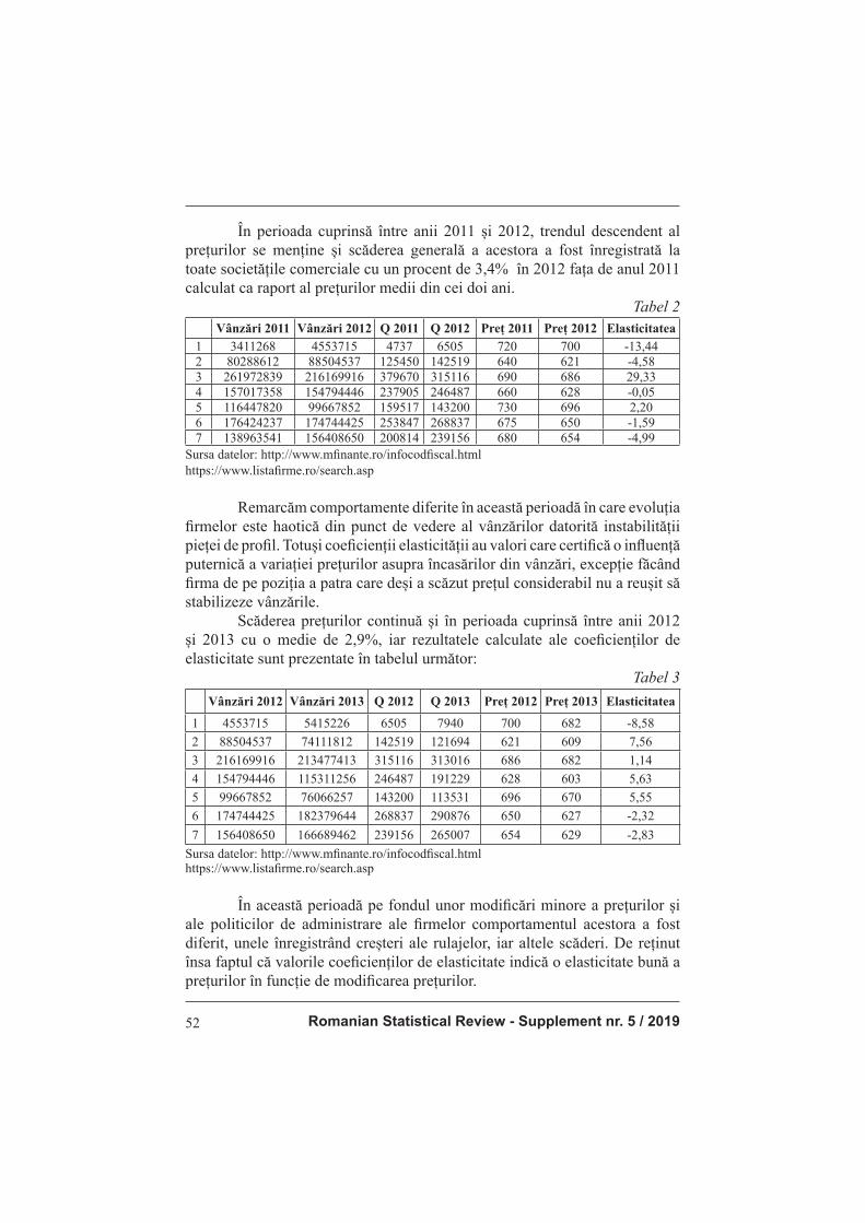
Romanian Statistical Review - Supplement nr. 5 / 201952
În perioada cuprinsă între anii 2011 și 2012, trendul descendent al prețurilor se menține și scăderea generală a acestora a fost înregistrată la toate societățile comerciale cu un procent de 3,4% în 2012 fața de anul 2011 calculat ca raport al prețurilor medii din cei doi ani.
Tabel 2
Vânzări 2011 Vânzări 2012 Q 2011 Q 2012 Preț 2011 Preț 2012 Elasticitatea1 3411268 4553715 4737 6505 720 700 -13,442 80288612 88504537 125450 142519 640 621 -4,583 261972839 216169916 379670 315116 690 686 29,334 157017358 154794446 237905 246487 660 628 -0,055 116447820 99667852 159517 143200 730 696 2,206 176424237 174744425 253847 268837 675 650 -1,597 138963541 156408650 200814 239156 680 654 -4,99
Sursa datelor: http://www.mfi nante.ro/infocodfi scal.htmlhttps://www.listafi rme.ro/search.asp
Remarcăm comportamente diferite în această perioadă în care evoluția fi rmelor este haotică din punct de vedere al vânzărilor datorită instabilității pieței de profi l. Totuși coefi cienții elasticității au valori care certifi că o infl uență puternică a variației prețurilor asupra încasărilor din vânzări, excepție făcând fi rma de pe poziția a patra care deși a scăzut prețul considerabil nu a reușit să stabilizeze vânzările. Scăderea prețurilor continuă și în perioada cuprinsă între anii 2012 și 2013 cu o medie de 2,9%, iar rezultatele calculate ale coefi cienților de elasticitate sunt prezentate în tabelul următor:
Tabel 3
Vânzări 2012 Vânzări 2013 Q 2012 Q 2013 Preț 2012 Preț 2013 Elasticitatea
1 4553715 5415226 6505 7940 700 682 -8,58
2 88504537 74111812 142519 121694 621 609 7,56
3 216169916 213477413 315116 313016 686 682 1,14
4 154794446 115311256 246487 191229 628 603 5,63
5 99667852 76066257 143200 113531 696 670 5,55
6 174744425 182379644 268837 290876 650 627 -2,32
7 156408650 166689462 239156 265007 654 629 -2,83
Sursa datelor: http://www.mfi nante.ro/infocodfi scal.htmlhttps://www.listafi rme.ro/search.asp
În această perioadă pe fondul unor modifi cări minore a prețurilor și ale politicilor de administrare ale fi rmelor comportamentul acestora a fost diferit, unele înregistrând creșteri ale rulajelor, iar altele scăderi. De reținut însa faptul că valorile coefi cienților de elasticitate indică o elasticitate bună a prețurilor în funcție de modifi carea prețurilor.
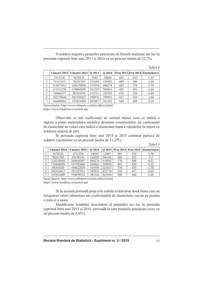
Revista Română de Statistică - Supliment nr. 5 / 2019 53
O scădere majoră a prețurilor practicate de fi rmele analizate are loc în perioada cuprinsă între anii 2013 și 2014 cu un procent mediu de 22,7%.
Tabel 4
Vânzări 2013 Vânzări 2014 Q 2013 Q 2014 Preț 2013 Preț 2014 Elasticitatea
1 5415226 5678326 7940 10050 682 565 -1,552 74111812 78251395 121694 156502 609 500 -1,603 213477413 228158884 313016 400278 682 570 -1,704 115311256 139866950 191229 284861 603 491 -2,645 76066257 98365630 113531 185595 670 530 -3,046 182379644 201936427 290876 395953 627 510 -1,947 166689462 193823809 265007 381542 629 508 -2,29
Sursa datelor: http://www.mfi nante.ro/infocodfi scal.htmlhttps://www.listafi rme.ro/search.asp
Observăm ca toți coefi cienții au semnul minus ceea ce indică o reglare a pieței materialelor metalice destinate construcțiilor, iar coefi cienții de elasticitate au valori care indică o elasticitate bună a vânzărilor în raport cu scăderea majoră de preț. În perioada cuprinsă între anii 2014 și 2015 continuă politica de scădere a prețurilor cu un procent mediu de 11,25%.
Tabel 5
Vânzări 2014 Vânzări 2015 Q 2014 Q 2015 Preț 2014 Preț 2015 Elasticitatea1 5678326 6711220 10050 12807 565 524 -3,782 78251395 93158145 156502 206102 500 452 -3,33 228158884 204649507 400278 410942 570 498 -0,214 139866950 155782886 284861 354858 491 439 -2,325 98365630 104822820 185595 223027 530 470 -1,786 201936427 193187951 395953 422730 510 457 -0,657 193823809 194839532 381542 423564 508 460 -1,66
Sursa datelor: http://www.mfi nante.ro/infocodfi scal.htmlhttps://www.listafi rme.ro/search.asp
Și în această perioadă piața este stabilă având doar două fi rme care au
înregistrat valori subunitare ale coefi cienților de elasticitate, cea de pe poziția
a treia și a șasea.
Modifi carea trendului descendent al prețurilor are loc în perioada
cuprinsă între anii 2015 și 2016, perioadă în care prețurile practicate cresc cu
un procent mediu de 4,45%.

Romanian Statistical Review - Supplement nr. 5 / 201954
Tabel 6
Vânzări 2015 Vânzări 2016 Q 2015 Q 2016 Preț 2015 Preț 2016 Elasticitatea
1 6711220 7087111 12807 12655 524 560 -0,17
2 93158145 87449415 206102 185667 452 471 -2,36
3 204649507 178183553 410942 350065 498 509 -6,71
4 155782886 152507879 354858 330103 439 462 -1,33
5 104822820 89883000 223027 183434 470 490 -4,17
6 193187951 179931955 422730 378804 457 475 -2,64
7 194839532 170375048 423564 354948 460 480 -3,73
Sursa datelor: http://www.mfi nante.ro/infocodfi scal.html
https://www.listafi rme.ro/search.asp
În aceasta perioada semnul și nivelul elasticității se păstrează cu o singură excepție și anume a fi rmei de pe poziția unu, fi rma care este cea mai mică din grupul celor analizate având un volum al vânzărilor cu un ordin de mărime mai mic decât celelalte. Consider că dimensiunea fi rmei a făcut difi cilă tranziția de la scăderea prețurilor la o nouă etapa în care acestea cresc. În perioada următoare aferente intervalului cuprins între anii 2016 și 2017 creșterea prețurilor este mai puternică cu o medie de 23,73%.
Tabel 7
Vânzări 2016 Vânzări 2017 Q 2016 Q 2017 Preț 2016 Preț 2017 Elasticitatea
1 7087111 6360841 12655 9637 560 660 -1,33
2 87449 415 109996210 185667 189648 471 580 0,09
3 178183 553 230745448 350065 378271 509 610 0,40
4 152507879 198824640 330103 334159 462 595 0,04
5 89883000 107192337 183434 175725 490 610 -0,17
6 179931955 198285930 378804 330476 475 600 -0,48
7 170375048 216298398 354948 354587 480 610 -0,01
Sursa datelor: http://www.mfi nante.ro/infocodfi scal.htmlhttps://www.listafi rme.ro/search.asp
În această perioadă întâmpinăm o creștere accelerată a prețurilor și modifi cări infi me ale cifrelor de afaceri care au distorsionat piața de profi l, iar valorile coefi cienților de elasticitate indică acest aspect atât prin natura semnului (plus și minus) cât și prin valorile subunitare înregistrate în ultima coloană a tabelului.
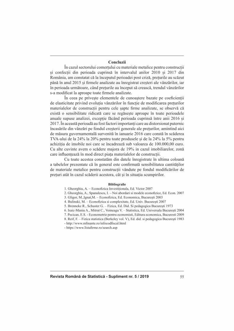
Revista Română de Statistică - Supliment nr. 5 / 2019 55
Concluzii În cazul sectorului comerțului cu materiale metalice pentru construcții și confecții din perioada cuprinsă în intervalul anilor 2010 și 2017 din România, am constatat că la începutul perioadei post criză, prețurile au scăzut până în anul 2015 și fi rmele analizate au înregistrat creșteri ale vânzărilor, iar în perioada următoare, când prețurile au început să crească, trendul vânzărilor s-a modifi cat la aproape toate fi rmele analizate. În ceea pe privește elementele de cunoaștere bazate pe coefi cienții de elasticitate privind evoluția vânzărilor în funcție de modifi carea prețurilor materialelor de construcții pentru cele șapte fi rme analizate, se observă că există o sensibilitate ridicată care se regăsește aproape în toate perioadele anuale supuse analizei, excepție făcând perioada cuprinsă între anii 2016 și 2017. În această perioadă au fost factori importanți care au distorsionat puternic încasările din vânzări pe fondul creșterii generale ale prețurilor, amintind aici de măsura guvernamentală survenită în ianuarie 2016 care constă în scăderea TVA-ului de la 24% la 20% pentru toate produsele și de la 24% la 5% pentru achiziția de imobile noi care se încadrează sub valoarea de 100.000,00 euro. Cu alte cuvinte avem o scădere majora de 19% in cazul imobiliarelor, zonă care infl uențează în mod direct piața materialelor de construcții. Cu toate acestea constatăm din datele înregistrate în ultima coloană a tabelelor prezentate că în general este confi rmată sensibilitatea cantităților de materiale metalice pentru construcții vândute pe fondul modifi cărilor de prețuri atât în cazul scăderii acestora, cât și în situația scumpirilor.
Bibliografi e
1. Gheorghiu, A. – Econofi zica Investiționala, Ed. Victor 2007 2. Gheorghiu, A., Spanulescu, I. – Noi abordari si modele econofi zice, Ed. Econ. 2007 3. Gligor, M.,Ignat,M. – Econofi zica, Ed. Economica, București 2003 4. Bulinski, M. – Econofi zica si complexitate, Ed. Univ. București 2007 5. Brenneke R., Schuster G. – Fizica, Ed. Did. Si pedagogica București 1973 6. Isaic-Maniu A., Mitrut C., Voineagu V. – Statistica, Ed. Universala București 2004 7. Pecican, E.S. - Econometrie pentru economisti, Editura economica, Bucuresti 2009 8. Reif, F. – Fizica statistica (Berkeley vol. V), Ed. did. si pedagogica București 1983 - http://www.mfi nante.ro/infocodfi scal.html - https://www.listafi rme.ro/search.asp
Romanian Statistical Review - Supplement nr. 5 / 201956
ANALYSIS MODEL OF THE POST-CRISIS BEHAVIOR OF THE COMPANIES
Ștefan Virgil Iacob PhD ([email protected])
Abstract
The period preceding the economic crisis of 2008 and 2009 was
marked by uncertainty regarding the price of promotion and sale of products
characteristic of the construction materials market in Romania. Since 2010,
the price of construction materials decreased steadily but also experienced
steep slopes that aff ected the activity of manufacturers, importers and
distributors in the fi eld.
The analysis is focused on the timeframe between 2010 and 2017. Thus,
during this time there have been periods of continuous price declines, such as
the years in which the blockade of buildings has led to the cessation of new
constructions and the freezing of some in diff erent phases of construction. The
declining values recorded in the fi rst years post-crisis were of a relatively small
intensity, ranging from 3 to 7%, followed by signifi cant decreases such as those
between 2013 and 2014, which recorded lower values by 22.7%. Minimum price
values were recorded in 2015 reaching an average of 471 euro / ton, followed by
price increases. Thus, between the years 2015 and 2016, there was an average
increase of 4.67%, and between 2016 and 2017 there was an average increase
of 23.73%. The upward trend in prices has been preserved so far.
Between 2014 and 2015, prices fl uctuated with oscillating low-
intensity behavior directly aff ecting economic activity, so the purchasing of
marketed materials became more and more diffi cult for local entrepreneurs.
In this research I have proposed to analyze aspects concerning the
sensitivity of demand for construction products in relation to price changes in
the period 2010-2017.
The fi eld of application of the study is represented by the companies in
the fi eld of trade in materials for light, medium and heavy metal constructions
and assets during the period mentioned. Seven commercial companies with
diff erent sales volumes were introduced into the analysis. These fall into two
categories: small fi rms with turnover below 100,000,000 lei / year and large
commercial companies with turnover of more than 100,000,000 lei / year.
The products that characterize this commercial area with direct
implications in the construction and real estate market in general are wire and
wire mesh for reinforcements, longitudinally welded or laminated, rectangular
or rounded pipes, cornier, tee, plate, strip and table profi les in various shapes
and sizes, black or thermally galvanized against corrosion.
Revista Română de Statistică - Supliment nr. 5 / 2019 57
Following the analysis, I highlighted the fact that there is a high
demand sensitivity in terms of price changes. The level of elasticity is
maintained over time, both in the period when prices decrease and the period
when metal products for construction increased. Also, the levels recorded by
the coeffi cients of elasticity in diff erent economic conditions characterizing the analyzed period are also quantifi ed. Keywords: price, sales, quantity of goods, coeffi cients, elasticity, sensitivity JEL Classifi cation: C01, L11, L61
Introduction
With a view to analyze the behavior of post-crisis metal building
materials distribution companies, I will address the issue of the variance in
sales revenue that these companies have in terms of the sales price of these
specifi c products for each year.
The method used is based on the elasticity of demand in relation to the
price.
I mentioned that the concept of elasticity comes from physics, where
this term is used to describe the property that the body possesses to resume its
original form after the action of an external force that altered it. (Brenneke, R.,
Schuster, G., 1973)
From the multitude of studies I mention the American economist A.
Marshall (1890), who took over the term elasticity in the language of physics and
diverted its core meaning. Thus, in economic studies, the elasticity coeffi cient
provides a way to measure the variation in demand depending on the price variation.
The meanings in physics and economy have nothing in common except, perhaps,
the initial reaction of the variable as an eff ect on the modifi cation of a factor.
In general, the concept of elasticity in the economy is used in the
analysis of demand for consumer goods. In Romanian literature one of the
initiators of the use of the concept of elasticity, as well as of other quantitative
methods, was Demetrescu M.C. (1971).
Pecican E.S. (2009) points out in his paper that the estimation of
regression parameters is recommended in the appreciation of the role of the
factors but considers that from the point of view of the elasticity it is important
to identify the sensitivity of the eff ect in relation to the factor / factors change.
So if in physics elasticity is a concept used to describe the property
that the body possesses to resume the initial form that the action of an external
force has altered, as soon as it stops its action, in the economy elasticity is
a measure of variation percentage of a variable in relation to the percentage
change of another variable considered as a factor.
Romanian Statistical Review - Supplement nr. 5 / 201958
Generally, estimates of elasticity are made for very small variations
of variables from where we bring the term of sensitivity into question. I also
mention that there may be an interest in the situation of the sensitivity of the
quantity required by a good to the change in the price of another good (cross-
elasticity).
Literature review Gheorghiu, A. (2007) classifi es diff erent economic models and uses
a series of physical models to analyze economic phenomena. Gheorghiu, A.,
Spanulescu, I. (2007) studied aspects related to the application of physics and
mathematics in economic theories. Gligor, M., Ignat, M. (2003) analyzed the
applications of theoretical physics in macroeconomic modeling. Bulinski,
M. (2007) addresses the fi eld of economics. Isaic-Maniu A., Mitrut C.,
Voineagu V. (2004) analyze the clues and calculates them as the average
ratio, the value of the value, the physical volume and the prices. The elasticity
study was approached by Pecican E.S. (2009) who analyzes the export and
import elasticity of Romania in the period between 1997 and 2002, taking
into account the exchange rate indicator that had signifi cant increases in the
analyzed period.
Methodology, data, results and discussions In order to study the behavior of post-crisis construction metal
distributors, we will consider two dependent indicators, namely the quantity
of products sold and the price for the promotion and sale of metallic materials.
We are going to calculate the elasticity coeffi cients for each fi rm and for each
annual period.
Thus, according to the economic theory, the price elasticity of the
demand is the sensitivity of the variance of the required quantity of a good in
relation to its price and is given by the relation:
5��=�
���������
����������=�
��
���
�����
���������������������������������������������������
�
�������� ��������
� � �
� � �
� � �
�� ���������� �������� �� �
� � �
[1]
where: = variation;
Pi și Qi = price and quantity of the good i;
If Δ is small I refer to the punctual elasticity of the demand, and if Δ is large, I talk about the sensitivity of the demand in response to the respective price change, which is known as the spring elasticity of the demand. According to the above, the analysis starts from the relationship:

Revista Română de Statistică - Supliment nr. 5 / 2019 59
5��=�
�� ���
��
�
�� ���������
���������������������������������������������������
�������� ��������
� � �
� � �
� � �
�� ���������� ��������
� � �
[2]
where: Q = the quantity of metal products sold
P = the promotion and sales price
The period between 2010 and 2011 is characterized by the overall
decrease of the prices recorded for all the analyzed companies by a percentage
average of 6.8% in 2011 compared to 2010. The reporting was made taking into account the average selling price registered in 2011 compared to the average sales price of the analyzed companies in 2010.
Table 1
Sales 2010 Sales 2011 Q 2010 Q 2011 Price 2010 Price 2011 Elasticity1 2327165 3411268 3022 4737 770 720 -8,742 58162590 80288612 84293 125450 690 640 -6,743 236385913 261972839 321613 379670 735 690 -2,954 133443666 157017358 187948 237905 710 660 -3,775 132978739 116447820 170485 159517 780 730 1,006 135206317 176424237 185214 253847 720 675 -5,927 100268661 138963541 136792 200814 725 680 -7,54
Data source: http://www.mfi nante.ro/infocodfi scal.htmlhttps://www.listafi rme.ro/search.asp
Analyzing the data from the period between 2010 and 2011 amid the fall in prices, the following can be noted: with only one exception (the fi fth company), all the companies registered increases in the quantity and, implicitly, in the volume of work. After computing the coeffi cient of elasticity, I fi nd absolute values
above the absolute, which shows that the sales are elastic in relation to the
price of all the companies under analysis.
The negative sign is the one expected given the reverse-to-sales
relationship between prices and sales.
At the limit, there is the company ranked fi fth, with turnover declines,
with the rest of the companies having a high sensitivity in terms of price
changes.
The average elasticity for the companies analyzed during this period
is -5.24, which confi rms a high general sensitivity of demand in line with price
changes.
Between 2011 and 2012, the downward trend in prices is maintained
and their overall decrease was recorded for all companies by 3.4% in 2012 compared to 2011 as a ratio of average prices in the two years.
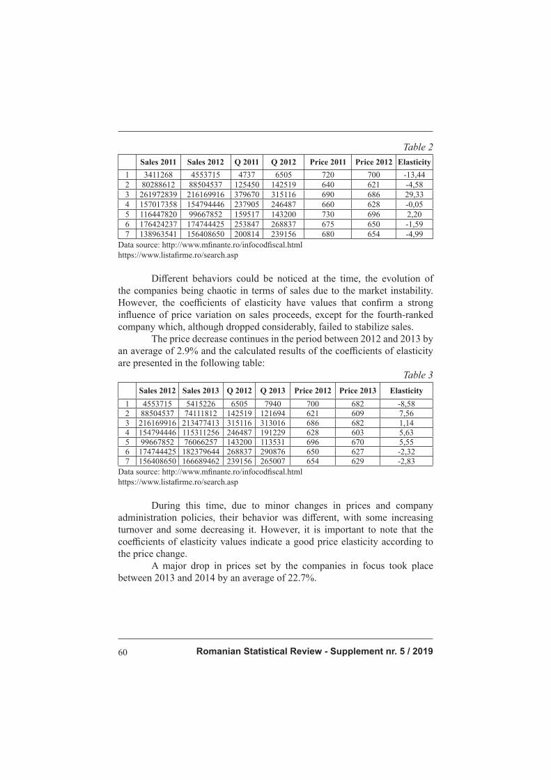
Romanian Statistical Review - Supplement nr. 5 / 201960
Table 2
Sales 2011 Sales 2012 Q 2011 Q 2012 Price 2011 Price 2012 Elasticity
1 3411268 4553715 4737 6505 720 700 -13,44
2 80288612 88504537 125450 142519 640 621 -4,58
3 261972839 216169916 379670 315116 690 686 29,33
4 157017358 154794446 237905 246487 660 628 -0,05
5 116447820 99667852 159517 143200 730 696 2,20
6 176424237 174744425 253847 268837 675 650 -1,59
7 138963541 156408650 200814 239156 680 654 -4,99
Data source: http://www.mfi nante.ro/infocodfi scal.html
https://www.listafi rme.ro/search.asp
Diff erent behaviors could be noticed at the time, the evolution of
the companies being chaotic in terms of sales due to the market instability.
However, the coeffi cients of elasticity have values that confi rm a strong
infl uence of price variation on sales proceeds, except for the fourth-ranked company which, although dropped considerably, failed to stabilize sales. The price decrease continues in the period between 2012 and 2013 by an average of 2.9% and the calculated results of the coeffi cients of elasticity
are presented in the following table:
Table 3
Sales 2012 Sales 2013 Q 2012 Q 2013 Price 2012 Price 2013 Elasticity
1 4553715 5415226 6505 7940 700 682 -8,58
2 88504537 74111812 142519 121694 621 609 7,56
3 216169916 213477413 315116 313016 686 682 1,14
4 154794446 115311256 246487 191229 628 603 5,63
5 99667852 76066257 143200 113531 696 670 5,55
6 174744425 182379644 268837 290876 650 627 -2,32
7 156408650 166689462 239156 265007 654 629 -2,83
Data source: http://www.mfi nante.ro/infocodfi scal.html
https://www.listafi rme.ro/search.asp
During this time, due to minor changes in prices and company
administration policies, their behavior was diff erent, with some increasing
turnover and some decreasing it. However, it is important to note that the
coeffi cients of elasticity values indicate a good price elasticity according to
the price change.
A major drop in prices set by the companies in focus took place
between 2013 and 2014 by an average of 22.7%.

Revista Română de Statistică - Supliment nr. 5 / 2019 61
Table 4
Sales 2013 Sales 2014 Q 2013 Q 2014 Price 2013 Price 2014 Elasticity1 5415226 5678326 7940 10050 682 565 -1,552 74111812 78251395 121694 156502 609 500 -1,603 213477413 228158884 313016 400278 682 570 -1,704 115311256 139866950 191229 284861 603 491 -2,645 76066257 98365630 113531 185595 670 530 -3,046 182379644 201936427 290876 395953 627 510 -1,947 166689462 193823809 265007 381542 629 508 -2,29
Data source: http://www.mfi nante.ro/infocodfi scal.html
https://www.listafi rme.ro/search.asp
As can be observed in table above, all coeffi cients have the minus
sign indicating a market regulation of building materials and the elasticity
coeffi cients have values that indicate a good sales elasticity in relation to the
major price drop.
Between 2014 and 2015, the pricing policy continues with an average
of 11.25%.Table 5
Sales 2014 Sales 2015 Q 2014 Q 2015 Price 2014 Price 2015 Elasticity1 5678326 6711220 10050 12807 565 524 -3,782 78251395 93158145 156502 206102 500 452 -3,33 228158884 204649507 400278 410942 570 498 -0,214 139866950 155782886 284861 354858 491 439 -2,325 98365630 104822820 185595 223027 530 470 -1,786 201936427 193187951 395953 422730 510 457 -0,657 193823809 194839532 381542 423564 508 460 -1,66
Data source: http://www.mfi nante.ro/infocodfi scal.html
https://www.listafi rme.ro/search.asp
At this time, the market is stable with just two companies registering
sub-unit values of the coeffi cients of elasticity, the third and sixth positions.
The change in the downward trend of prices takes place between 2015
and 2016, during which the prices are rising by an average of 4.45%.
Table 6
Sales 2015 Sales 2016 Q 2015 Q 2016 Price 2015 Price 2016 Elasticity
1 6711220 7087111 12807 12655 524 560 -0,172 93158145 87449415 206102 185667 452 471 -2,363 204649507 178183553 410942 350065 498 509 -6,714 155782886 152507879 354858 330103 439 462 -1,335 104822820 89883000 223027 183434 470 490 -4,176 193187951 179931955 422730 378804 457 475 -2,647 194839532 170375048 423564 354948 460 480 -3,73
Data source: http://www.mfi nante.ro/infocodfi scal.htmlhttps://www.listafi rme.ro/search.asp
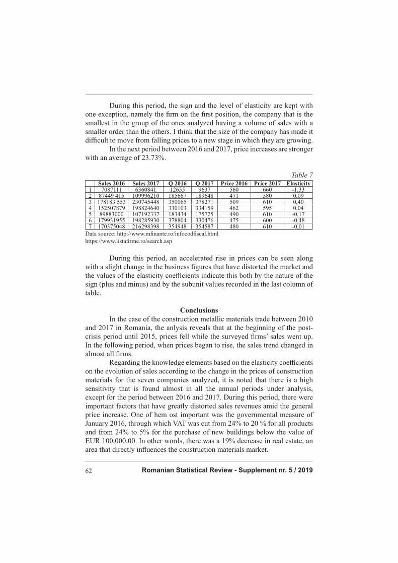
Romanian Statistical Review - Supplement nr. 5 / 201962
During this period, the sign and the level of elasticity are kept with
one exception, namely the fi rm on the fi rst position, the company that is the
smallest in the group of the ones analyzed having a volume of sales with a
smaller order than the others. I think that the size of the company has made it
diffi cult to move from falling prices to a new stage in which they are growing.
In the next period between 2016 and 2017, price increases are stronger
with an average of 23.73%.
Table 7 Sales 2016 Sales 2017 Q 2016 Q 2017 Price 2016 Price 2017 Elasticity1 7087111 6360841 12655 9637 560 660 -1,332 87449 415 109996210 185667 189648 471 580 0,093 178183 553 230745448 350065 378271 509 610 0,404 152507879 198824640 330103 334159 462 595 0,045 89883000 107192337 183434 175725 490 610 -0,176 179931955 198285930 378804 330476 475 600 -0,487 170375048 216298398 354948 354587 480 610 -0,01
Data source: http://www.mfi nante.ro/infocodfi scal.htmlhttps://www.listafi rme.ro/search.asp
During this period, an accelerated rise in prices can be seen along with a slight change in the business fi gures that have distorted the market and the values of the elasticity coeffi cients indicate this both by the nature of the
sign (plus and minus) and by the subunit values recorded in the last column of
table.
Conclusions In the case of the construction metallic materials trade between 2010
and 2017 in Romania, the anlysis reveals that at the beginning of the post-
crisis period until 2015, prices fell while the surveyed fi rms’ sales went up.
In the following period, when prices began to rise, the sales trend changed in
almost all fi rms.
Regarding the knowledge elements based on the elasticity coeffi cients
on the evolution of sales according to the change in the prices of construction
materials for the seven companies analyzed, it is noted that there is a high
sensitivity that is found almost in all the annual periods under analysis,
except for the period between 2016 and 2017. During this period, there were
important factors that have greatly distorted sales revenues amid the general
price increase. One of hem ost important was the governmental measure of
January 2016, through which VAT was cut from 24% to 20 % for all products and from 24% to 5% for the purchase of new buildings below the value of EUR 100,000.00. In other words, there was a 19% decrease in real estate, an area that directly infl uences the construction materials market.
Revista Română de Statistică - Supliment nr. 5 / 2019 63
However, according to the data recorded in the last column of the
tables, the sensitivity of the sold quantities of metallic building materials to
price changes is generally confi rmed both in the case of decrease and in the
case of increases.
Bibliography 1. Gheorghiu, A. – Econofi zica Investiționala, Ed. Victor 2007
2. Gheorghiu, A., Spanulescu, I. – Noi abordari si modele econofi zice, Ed. Econ. 2007
3. Gligor, M.,Ignat,M. – Econofi zica, Ed. Economica, București 2003
4. Bulinski, M. – Econofi zica si complexitate, Ed. Univ. București 2007
5. Brenneke R., Schuster G. – Fizica, Ed. Did. Si pedagogica București 1973
6. Isaic-Maniu A., Mitrut C., Voineagu V. – Statistica, Ed. Universala București 2004
7. Pecican, E.S. - Econometrie pentru economisti, Editura economica, Bucuresti 2009
8. Reif, F. – Fizica statistica (Berkeley vol. V), Ed. did. si pedagogica București 1983
- http://www.mfi nante.ro/infocodfi scal.html
- https://www.listafi rme.ro/search.asp
Romanian Statistical Review - Supplement nr. 5 / 201964
Static and Structural Analysis of Gross Domestic Product
Tudor SAMSON PhD Student ([email protected])
Bucharest University of Economic Studies
Alexandra PETRE (OLTEANU) PhD Student ([email protected])
Bucharest University of Economic Studies
Cristian OLTEANU PhD Student ([email protected])
Bucharest University of Economic Studies
Marin-Marius GĂNCIULESCU Master Student
Abstract In this article, the authors propose to realize an analysis of the concrete
results obtained by Romania in the fi rst quarter of 2019. The most complex
indicator associated with GDP per capita and purchasing power parity, is the
Gross Domestic Product, that express how the economic growth is achieved in
a country. In the case of Romania, as in other countries, according to Eurostat
methodology, analyzes are performed on a quarterly basis to identify trends in
the evolution of this macroeconomic indicators. As a Gross Domestic Product
the indicator calculated at one year level and the evolution of the gross domestic
situation the quarterly product is made in three phases, these data will be
successively corrected. In the article the authors present certain methodological
aspects related to signal estimates and preliminary estimates to provide a
correct image of Romania’s economic evolution.The authors also point out that
the signal produced in the Romanian national accounts are obtained by use of
the direct method, when applied to the existence of sub-annual data sources
and here we have as example statistical surveys and other data that permits
calculation of this indicator. This method is used to calculate this indicator,
based on the gross value added to the basic price used in the economy.
The authors continue to analyze how gross domestic product evolved
in the fi rst quarter of 2019, compared with the evolution of gross domestic
product on the same quarter for a longer period between 2015 and 2018. The
comparison is also based on gross series, as well as on the seasonally adjusted
series. To highlight evolution of this indicator, this evolution is graphically
presented between 2000 and 2018. It should be noted that, 2008-2012 was a
crisis period and the upward trend stared with 2013.
Keywords: GDP, fi nal consumption, net exports, investment,
evolution
JEL Classifi cation: E01, E21

Revista Română de Statistică - Supliment nr. 5 / 2019 65
Introduction The analysis of the Gross Domestic Product evolution on a quarterly
basis in 2019 in real terms, starts from the quarterly calculation of this indicator
in order to draw useful conclusions for macroeconomic management in order
to have the possibility to take additional measures if the evolution of the
indicator show declining tendencies. Firstly in this article, the methodological
aspects of signal estimations and provisional estimates are presented to give
the reader the opportunity to understand the content. On the basis of relative
fi gures, an analysis is made of how this indicator has developed quarterly over
a period of 4 years, 2015-2018, and for more prominent use the graphical
representation was used for a period of 19 years, from 2000 until 2018. Graphic
representation is suggestive, pointing to a downward trend after 2007-2008 of
quarterly gross domestic product, which in 2013 only resumed its growth rate,
which is currently maintaining a marked trend in 2015, being enlightening in
this it means that in the third quarter of 2017, growth over the corresponding
quarter of 2016 was 8.8% on the gross series and 8.6% on the seasonally
adjusted series. The article refers to some quarters in which growth has had
a greater signifi cance, giving some suggestions, which should be taken into
considered by macroeconomic management.
Literature review Anghel, Anghelache, Dumitrescu and Dumitrescu (2016) used the
econometric tools to study the correlation between Gross Domestic Product and
Foreign Direct Investment and net exports to Romania. Anghelache, Anghel,
Marinescu and Dumbravă (2018) have developed a study on the evolution
of GDP in Romania. Anghelache and Anghel (2017) used econometric tools
to study the factors of infl uence over GDP growth. Anghelache et al. (2016)
carried out a comparative analysis of the evolution of the Gross Domestic
Product indicator. Dumitrescu, Anghel, and Anghelache (2015) studied
the dependence of GDP on structural variables. Koulakiotis, Lyroudi and
Papasyriopoulos (2012) have studied the cause-eff ect relationship between
infl ation and GDP in fourteen European countries, they have emphasized a
two-ways interdependence between these macroeconomic variables, with a
level of signifi cance of 10%. Nalewaik (2012) researched the estimates of
GDP recession probabilities. Garin, Lester and Sims (2016) studied a number
of issues related to nominal GDP.
Research methodology, data, results and discussions In order to understand how the national economy evolved the GDP
Analysis is an important tool, which can ensure the control and tracking of the
Romanian Statistical Review - Supplement nr. 5 / 201966
economy evolution. By using these short-term indicators, we can identify the
eff ect of the measures taken, as well as some shortcomings that may occur.
The “signal” estimates of the quarterly GDP are made in order to off er
the fastest image on the evolution of the economy and have the following
characteristics: they are produced and published no later than 45 days after the
end of the quarter; are in accordance with the National Accounts methodology;
are based on an incomplete set of information in comparison with the estimates
of the national account, including the GDP, thus being revised on a quarterly
basis. The diff erences between the two are that the “signal” estimates are
available faster than the GPD however they are not as accurate as the GDP.
The “signal” is available after 45 days and the GDP is available after 75 days.
Generally the „signal” estimates are not as accurate as the provisional
ones, however the loss in precision is intended to be minimized to the lowest
possible level. Estimation method: Depending on the available data sources,
the direct method (using existing data and estimations for non-available data)
or the indirect method (using regression techniques) can be used. Available
information: Signal estimates are based on a limited set of data. Often, some
information provided by statistical surveys or administrative sources is not
available. Scope of coverage: The number of variables covered by the „signal”
estimates is limited.
“Signal” estimates of the quarterly GDP in the Romanian national
accounts are carried out by applying the direct method given the existence
of infra-annual data sources, in particular investigations which provide
information that allows estimation of Gross Domestic Product quarterly
(PIBT) at market price by the production method, according to the following
relationship:
PIBT = VAB + IP – SP
where:
VAB = Gross Value Added at Base Price;
IP = taxes on product;
SP = subsidies on product.
The comparison of Gross Domestic Product (GDP) quarterly compared
to the same period of the previous year, seasonally adjusted estimates are
also calculated using the regressive method, a method recommended by the
European regulations, which compares PIBT in two consecutive quarters.
To highlight the real world economic developments seasonal
adjustments can be used to mitigate the eff ects in the data series.
Romania’s quarterly national accounts tend to show a strong seasonality
and are also adjusted to the number of working days and the calendar, if this
eff ect is negligible. The seasonally adjusted series was obtained by removing
Revista Română de Statistică - Supliment nr. 5 / 2019 67
the seasonal eff ect by using the correction coeffi cients, based on the regression
model used (additive or multiplicative). The additive or multiplicative model
used for the regression is automatically identifi ed by the Demetra program
according to the type of series used. The seasonally adjusted time series of the
last 5 years and the available quarters of the reference year are recalculated
quarterly, the quarterly and annual series of revisions of the unadjusted series
following available for further statistical and administrative data sources with
a higher coverage accuracy of the last available observation in the dataset,
change of inherited models and regression parameters.
The DEMETRA program package (TRAMO / SEATS method) is
used to adapt the main aggregate series on the basis of which GDP is estimated
by using production method and expenditure method. It estimates the seasonal
eff ect (events occurring at the same time, with the same strength and direction
each year as the seasons, holidays, etc., the number of working days that diff er
from one month to the next and the eff ect of the calendar). such as Orthodox
Easter, bisect year and other national holidays), as well as the detection and
correction of extreme values (occasional, temporary or permanent changes)
and the interpolation of missing values.
By looking at the information provided, it can be seen that the GDP in
the last quarter had a positive evolution of 4.1% in gross series, compared to
the same period of last year.
Also the evolution of the GDP seasonally adjusted series has shown
that there is indeed a positive evolution of the GDP of approximately 4%.
The evolution of the Gross Domestic Product quarterly between 2016
and 2018, calculated as gross series and seasonally adjusted series, presented
in table no. 1 points out that in 2018, Gross Domestic Product recorded
successive increases, both on gross series and seasonally adjusted series.
Thus, in both situations, the increases were similar, namely 4.0% in the fi rst
quarter, 4.1% in the second quarter, 4.2.% in the third quarter and 4.1 in the
last quarter, respectively, in the gross series and 4.5% in the fi rst quarter , 4.3%
in the second quarter, 3.8% in the third quarter and 4.0% in the last quarter,
based on the seasonally adjusted series.
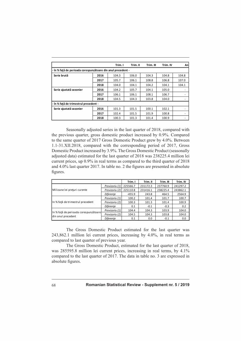
Romanian Statistical Review - Supplement nr. 5 / 201968
Trim. I Trim. II Trim. III Trim. IV An
Serie brută 2016 104.3 106.0 104.3 104.8 104.8
2017 105.7 106.1 108.8 106.8 107.0
2018 104.0 104.1 104.2 104.1 104.1
Serie ajustată sezonier 2016 104.2 105.7 104.1 105.0 -
2017 106.1 106.1 108.1 106.7 -
2018 104.5 104.3 103.8 104.0 -
Serie ajustată sezonier 2016 101.3 101.5 100.1 102.1 -
2017 102.4 101.5 101.9 100.8 -
2018 100.3 101.3 101.4 100.9 -
- în % faţă de perioada corespunzătoare din anul precedent -
- în % faţă de trimestrul precedent -
Seasonally adjusted series in the last quarter of 2018, compared with
the previous quarter, gross domestic product increased by 0.9%. Compared
to the same quarter of 2017 Gross Domestic Product grew by 4.0%. Between
1.1-31.XII.2018, compared with the corresponding period of 2017, Gross
Domestic Product increased by 3.9%. The Gross Domestic Product (seasonally
adjusted data) estimated for the last quarter of 2018 was 238225.4 million lei
current prices, up 0.9% in real terms as compared to the third quarter of 2018
and 4.0% last quarter 2017. In table no. 2 the fi gures are presented in absolute
fi gures.
Trim. I Trim. II Trim. III Trim. IV
Provizoriu (1) 225566.7 231172.3 237760.9 241297.2
Provizoriu (2) 225110.8 231416.1 238225.4 243862.1
Diferenţe -455.9 243.8 464.5 2564.9
Provizoriu (1) 100.2 101.4 101.7 100.7
Provizoriu (2) 100.3 101.3 101.4 100.9
Diferenţe 0.1 -0.1 -0.3 0.2
Provizoriu (1) 104.4 104.3 103.9 104.0
Provizoriu (2) 104.5 104.3 103.8 104.0
Diferenţe 0.1 0.0 -0.1 0.0
In % faţă de perioada corespunzătoare
din anul precedent
Milioane lei preţuri curente
In % faţă de trimestrul precedent
The Gross Domestic Product estimated for the last quarter was
243,862.1 million lei current prices, increasing by 4.0%, in real terms as
compared to last quarter of previous year.
The Gross Domestic Product, estimated for the last quarter of 2018,
was 285595.8 million lei current prices, increasing in real terms, by 4.1%
compared to the last quarter of 2017. The data in table no. 3 are expressed in
absolute fi gures.
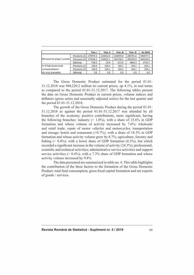
Revista Română de Statistică - Supliment nr. 5 / 2019 69
Trim. I Trim. II Trim. III Trim. IV An 2018
Provizoriu (1) 179974.3 216652.0 263059.6 280791.6 940477.5
Provizoriu (2) 179246.1 216632.1 262746.2 285595.8 944220.2
Diferenţe -728.2 -19.9 -313.4 4804.2 3742.7
Provizoriu (1) 104.0 104.1 104.2 104.1 104.1
Provizoriu (2) 104.0 104.1 104.2 104.1 104.1
Diferenţe 0.0 0.0 0.0 0.0 0.0
In % faţă de perioada
corespunzătoare
din anul precedent
Milioane lei preţuri curente
The Gross Domestic Product estimated for the period 01.01-
31.12.2018 was 944,220.2 million lei current prices, up 4.1%, in real terms
as compared to the period 01.01-31.12.2017. The following tables present
the data on Gross Domestic Product in current prices, volume indices and
defl ators (gross series and seasonally adjusted series) for the last quarter and
the period 01.01-31.12.2018.
The growth of the Gross Domestic Product during the period 01.01-
31.12.2018 as against the period 01.01-31.12.2017 was attended by all
branches of the economy, positive contributions, more signifi cant, having
the following branches: industry (+ 1.0%), with a share of 23.6% in GDP
formation and whose volume of activity increased by 7.6%; wholesale
and retail trade; repair of motor vehicles and motorcycles; transportation
and storage; hotels and restaurants (+0.7%), with a share of 18.3% in GDP
formation and whose activity volume grew by 8.7%; agriculture, forestry and
fi shing (+ 0.4%), with a lower share of GDP formation (4.3%), but which
recorded a signifi cant increase in the volume of activity (24.3%); professional,
scientifi c and technical activities; administrative service activities and support
service activities (+ 0.4%), with a 7.3% share of GDP formation and whose
activity volume increased by 9.8%.
The data presented are summarized in table no. 4. This table highlights
the contribution of the three factors to the formation of the Gross Domestic
Product: total fi nal consumption, gross fi xed capital formation and net exports
of goods / services.

Romanian Statistical Review - Supplement nr. 5 / 201970
Provizoriu (1) Provizoriu (2) Provizoriu (1) Provizoriu (2)
Agricultură, si lvicultură şi pescuit 4.4 4.3 0.4 0.4
Industrie 23.7 23.6 1.0 1.0
Construcţii 5.4 5.4 -0.3 -0.3
Comerţ cu ridicata și cu amănuntul;
repararea autovehiculelor şi
motocicletelor; transport şi depozitare;
hoteluri şi restaurante 18.3 18.3 0.7 0.7
Informații și comunicații 5.2 5.2 0.4 0.4
Intermedieri financiare şi asigurări 2.7 2.7 0.0 0.0
Tranzacţii imobiliare 7.5 7.5 0.2 0.2
Activități profesionale, ști ințifice și
tehnice; activități de servicii
administrative și activități de servicii
suport 7.3 7.3 0.4 0.4
Administrație publică și apărare; asigurări
sociale din sistemul public; învățământ;
sănătate și asistență socială 12.9 13.1 0.2 0.2
Activități de spectacole, culturale și
recreative; reparații de produse de uz
casnic și alte servicii 3.1 3.0 0.1 0.1
Valoarea adăugată brută – total 90.5 90.4 3.1 3.1
Impozite nete pe produs 9.5 9.6 1.0 1.0
Produsul intern brut 100.0 100.0 4.1 4.1
Contribuţia la formarea PIB - % Contribuţia la creşterea PIB - %
From the GDP growth point of view, the increase was mainly due to
the fi nal consumption expenditure of households, whose volume increased by
9.7%, contributing + 3.3% to GDP growth.
A negative contribution to GDP growth was recorded by net exports
(-1.7%), as a result of the 9.6% increase in exports of goods and services
correlated with a higher increase in the volume of imports of goods and
services (10, 8%).

Revista Română de Statistică - Supliment nr. 5 / 2019 71
Provizoriu (1) Provizoriu (2) Provizoriu (1) Provizoriu (2)
Consumul final efectiv total 79.3 79.1 3.9 3.6
Consum final individual efectiv al
gospodării lor populaţiei 70.1 69.1 3.4 2.6
Cheltuiala pentru consumul final al
gospodării lor populaţiei 61.9 61.7 3.3 3.3
Cheltuiala pentru consumul final al
instituţii lor fără scop lucrativ în
serviciul gospodării lor populaţiei 0.8 0.8 0.0 0.0
Cheltuiala pentru consumul final
individual al administraţii lor publice 7.4 6.6 0.1 -0.7
Consumul final colectiv efectiv al
administraţii lor publice 9.2 10.0 0.5 1.0
Formarea brută de capital fix 21.3 21.2 -0.7 -0.7
Variaţia stocurilor 2.7 2.9 2.7 2.9
Exportul net de bunuri şi servicii -3.3 -3.2 -1.8 -1.7
Exportul de bunuri şi servicii 41.5 41.7 1.9 2.3
Importul de bunuri şi servicii 44.8 44.9 3.7 4.0
Produsul intern brut 100.0 100.0 4.1 4.1
Contributia la formarea PIB - % Contribuţia la creşterea PIB - %
The highest contribution for the 2018 GDP is based on the total fi nal
consumption, while the Net Export has a negative impact on the overall GDP
performance indicator. Moreover the GDP of 2018 reached 4.1% while the
GDP of 2017 reached 7.0% thus leading us to think that now the economy is
on a slow declining path.
Conclusion The author’s study concludes that in 2017, the upward trend in
quarterly growth of Gross Domestic Product continued. In spite of some
controversy over the way of economic growth, it is obvious that, even on
account of consumption, in the third quarter of 2017 Romania achieved the
highest quarterly growth rate across the European Union, as is the rest of
Europe. The second conclusion is that an increase in consumption is not
sustainable long-term growth and therefore measures must be taken to ensure
gross domestic product growth in the coming period and to capital investment,
creating new jobs , which also ensures the absorption of the unemployed
and the unoccupied population. In the immediate future, it is necessary to
use a mixed growth method, ie both consumption and investment. Increased
investment must be done by supporting domestic capital, attracting foreign
Romanian Statistical Review - Supplement nr. 5 / 201972
direct investment and accessing community funds. Another conclusion is that
in Romania there are a number of sectors of the national economy that have
to increase their contribution to the realization of the gross domestic product,
which is in a more delicate situation due to the lack of investments. Another
suggestion, and last, is that macroeconomic management needs to fi nd a
short, medium and long-term strategy with concrete measures implemented to
ensure growth in the next period. Some suggestions that a new economic and
fi nancial crisis might occur in Romania, or in Europe or around the world.
We need to learn from the last crisis 2008-2012 that a long-term adjustment
program for economic growth may be benefi cial for a country like Romania
that has much to do in a number of sectors, if not in all sectors of the national
economy.
References 1. Anghel, M.G., Anghelache, C., Dumitrescu, D.V., Dumitrescu, D. (2016). Analysis
of the correlation between the Gross Domestic Product and some factorial variable.
Romanian Statistical Review, Supplement, 10, 138-145
2. Anghelache, C., Anghel, M.G., Marinescu, A.I., Dumbravă, Ş.G. (2018). Complex
Analysis of Gross Domestic Product at the End of 2017. Romanian Statistical
Review, Supplement, 2, 132-139
3. Anghelache, C., Anghel, M.G. (2017). Econometric methods and models used
in the analysis of the factorial influence of the gross domestic product growth.
Network Intelligence Studies, V (9), 67-78
4. Anghelache, C. et al. (2016). Comparative study of the evolution of the Gross
Domestic Product indicator. Romanian Statistical Review Supplement, 12, 163-170
5. Dumitrescu, D., Anghel, M.G., Anghelache, C. (2015). Analysis Model of GDP
Dependence on the Structural Variables. Theoretical and Applied Economics, 22
(4), (605), Winter, 151-158
6. Koulakiotis, A., Lyroudi, K., Papasyriopoulos, N. (2012). Inflation, GDP and
Causality for European Countries. International Advances in Economic Research,
18 (1), 53-62
7. Nalewaik, J. (2012). Estimating Probabilities of Recession in Real Time with GDP
and GDI. Journal of Money, Credit and Banking, 44, 235-253
8. Garin, J., Lester, R., Sims, E. (2016). On the Desirability of Nominal GDP
Targeting. Journal of Economic Dynamics and Control, 69, 21–4
9. Institutul Național de Statistică, Comunicatul de presă nr. 54 / 7.03.2018
10. Institutul Național de Statistică, Comunicatul nr. 304/05.12.2017
11. Institutul Național de Statistică, Comunicatul nr. 294/14.11.2017

Revista Română de Statistică - Supliment nr. 5 / 2019 73
Migraţia economică – analiza factorilor determinanţi ai acesteia
Drd. Olivia –Georgiana NIȚĂ ([email protected])
Academia de Studii Economice din București
Drd. Alexandru BADIU ([email protected])
Academia de Studii Economice din București
Abstract Migrația poate fi descrisă ca un fenomen spațial, deoarece implică
schimbarea locului de rezidență al unei persoane, pe o perioadă variată
sau determinată de timp. Migrația presupune mișcarea populației, fi e că se
petrece în interiorul unei țări, fi e că are loc în afara granițelor unei țări.
Motivația unei persoane de a pleca din țara natală are la bază o combinație
de factori de natură economică, politică sau etnică. Se pot observa o serie
de factori atractivi care pot infl uența decizia migrantului de a pleca din țara
de origine, printre astfel de factori se numără: îmbunătățirea calității vieții,
dezvoltarea personală și profesională, precum și factori de natură politică,
cum ar fi : respectarea drepturilor, a legii și libertății, siguranță și securitate.
Cel mai mare impact însă, in luarea deciziei de a pleca din țara de origine
o au factorii de natură economică. Migrația este determinată de diferențele
salariale dintre două regiuni geografi ce, țara de origine a migrantului și țara
de destinație a acestuia. Acesta va analiza îndeaproape toate opțiunile sale
și o va alege pe cea care ii va maximiza utilitatea și îi va satisface nevoile
din momentul respectiv. Motivul principal pentru care migranții aleg să plece
temporar sau permanent din țara natală este cel de creștere a veniturilor.
Corelația directă și pozitivă dintre creșterea veniturilor migrantului și
îmbunătățirea calității vieții acestuia și implicit a familiei lui, accesul la
sisteme de sănătate mai bune, sisteme educaționale pentru copii, dezvoltarea
personală și profesională, precum și alte nevoi, infl uențează migrantul în
alegera unei noi destinații.
Cuvinte cheie: migrația, factori de infl uență, calitatea vieții,
motivație, diferențe salariale
Clasifi carea JEL: F22, O15
Introducere
Migrantul internațional este persoana ce locuiește într-o țară diferită de cea în care s-a născut. Motivul pentru care alege să plece din țara natală este legat de o serie de factori de infl uență, fi e din țara natală, fi e din țara

Romanian Statistical Review - Supplement nr. 5 / 201974
de destinație, factori de natură: economică, politică sau socială. Migrantul
economic sau lucrătorul migrant, așa cum mai este defi nit de Organizația Natiunilor Unite (ONU), este o persoană care își părăsește țara căutând o îmbunătățire a nivelului de trai sau oportunități de angajare, deoarece condițiile economice din țara sa nu sunt satisfăcătoare.
Literature review Anghel, Niță și Badiu (2017) au analizat efectul remitențelor asupra creșterii economice. O temă similară este studiată de Giuliano și Ruiz-Arranz (2009). Anghelache, Niță și Badiu (2017) au utilizat modele econometrice pentru a studia impactul remitențelor în economie. Anghelache (2009) a utilizat instrumentarul statistic pentru analiza migrației. Artjoms și King (2012), precum și Foley și Angjellari-Dajci au cercetat motivele migrației. Beets și Willekens, (2009) au studiat corelația dintre criza economică globală și migrația internatională. Crowder, Hall and Tolnay (2011) au analizat tipurile de migrație. Kaplan și Schulhofer-Wohl (2012) au studiat migrația transfrontalieră. Kennan și Walker (2011) au analizat infl uența venitului așteptat asupra deciziei de migrație. Moreno-Galbisa și Tritah (2016) au studiat efectele imigrației pe piețele forței de muncă. Zaiceva și Zimmermann (2013) au abordat aspect ale revenirii migranților în țara de origine.
Metodologia cercetării, date, rezultate și discuții
Banca Mondială grupează factorii care contribuie în luarea deciziei de a migra într-o altă țară în trei mari categorii și anume: 1. Factori economici și demografi ci. Aspectele analizate din punct de
vedere economic și demografi c care contribuie în mod semnifi cativ la adoptarea deciziei de a migra din țara de origine se referă la sărăcie; șomaj ridicat; salarii mici; taxe mari; rate de fertilitate crescute; sisteme de sănptate precare. Aspectele atractive ale migrării într-o altă țară vizează cerere de muncă; perspectiva unui salariu mai mare; potențial de îmbunătățire a standardului de viață; sisteme de educație și sănătate favorabile; creștere economică puternică; tehnologie.
2. Factori politici. În categoria factorilor presanți din punct de vedere politic se includ: confl ictul, nesiguranța, violența; guvernarea slabă; corupția; abuzurile drepturilor umane, iar în categoria celor atractivi “pull”: siguranța și securitatea; libertatea politică; drepturile și libertățile.
3. Sociali și culturali. Factorii presanți “push” din punct de vedere social și cultural cuprind discriminarea bazată pe etnie, gen, religie,
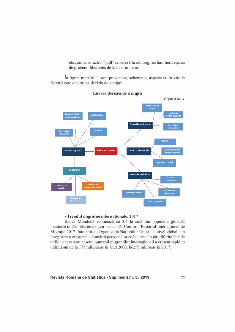
Revista Română de Statistică - Supliment nr. 5 / 2019 75
etc., iar cei atractivi “pull” se referă la reîntregirea familiei; rețeaua de prieteni; libertatea de la discriminare.
În fi gura numărul 1 sunt prezentate, schematic, aspecte cu privire la factorii care determină decizia de a migra.
Luarea deciziei de a migraFigura nr. 1
• Trendul migrației internaționale, 2017
Banca Mondială estimează că 3.4 la sută din populația globală, locuiește în țări diferite de țara lor natală. Conform Raportul Internațional de Migrație 2017 întocmit de Organizația Națiunilor Unite, la nivel global, s-a înregistrat o creșterea a numărul persoanelor ce locuiesc în țări diferite față de
țările în care s-au născut, numărul migranților internaționali a crescut rapid în
ultimii ani de la 173 milionane în anul 2000, la 258 milioane în 2017.

Romanian Statistical Review - Supplement nr. 5 / 201976
Evoluția numărului de migranți (milioane)Figura nr. 2
�
���� �������+������ 3���� 40� � �����4�����3��74�������8�
-69-;-
++5
+<=
+.=
)
D)
*))
*D)
())
(D)
;))
())) ())D ()*) ()*D ()()
Sursa de date: Organizația Națiunilor Unite
Același raport prezintă faptul că pe primele locuri în ceea ce privește continentele gazdă ale migrației internaționale se afl ă Asia cu 80 milioane și Europa cu 78 milioane, urmate de America de Nord cu 58 milioane și Africa cu 25 milioane.
Numărul migranților internaționali, după destinație (milioane)Figura nr. 3�
���� �������9��� 40� ��4�����3�������%����3������,�� :0���$%���3���
��
��
��
��
�� �
%��� F� ��
%����������� �� %�����
%�������G���������C�����3����#� �������
Sursa de date: Organizația Națiunilor Unite
În ceea ce privește orginea celor 258 milioane de migranți, 106 milioane dintre aceștia s-au născut în Asia, 61 milioane în Europa, 38 milioane în America Latină și Caraibe, 36 milioane în Africa.
Revista Română de Statistică - Supliment nr. 5 / 2019 77
Cifrele înregistrate în 2017 arată că în topul țărilor de origine a migranților internaționali se regăsesc India (17 milioane), Mexic (13 milioane), Federația Rusă (11 milioane), China (10 milioane), Bangladesh (7 milioane), Republica Arabă Siriană (7 milioane), Pakistan și Ucraina (6
milioane), România (3.6 milioane).
În anul 2017, 67% din migrația internațională era concentrată în 20 țări, Statele Unite ale Americii cu 50 milioane de migranți internaționali se afl ă în topul țărilor de destinație, pe locurile următoare fi ind Arabia Saudită, Germania și Federația Rusă, fi ecare găzduind în jur de 12 milioane migranți, Anglia și Irlanda de Nord, cu aproximativ 9 milioane fi ecare. În ceea ce privește numărul total al refugiaților și solicitanților de azil, numărul ofi cial înregistrat al acestora a fost în anul 2016 de 25,9 milioane. Turcia (3.1 milioane) găzduind cea mai mare parte a acestora, pe locul doi și trei regăsindu-se Iordania (2.9 milioane) și pe locul 3 Palestina (2.2 milioane). Obiectivul acestei lucrări însă este de a analiza impactul lucrătorilor migranți în țările de origine, cât și destinație. Așadar refugiații și solicitanții de azil nu fac parte din obiectul acestui studiu și nu vor fi incluși determinarea impactului migrației asupra dezvoltării economice a unei țări. Presupunem că motivul principal pentru migrației il reprezintă îmbunătățirea calității vieții a migrantului, cât și a familiei acestuia, migrantul internațional părăstește țara de origine din dorința de a-și acoperi nevoi ca: un loc de muncă mai bun, educație, sănătate. În ceea ce privește refugiații și solicitanții de azil, aceștia își părăsesc țările de origine mai ales din motive politice. Numărul mare al refugiaților din ultimii doi ani, consider că nu trebuie inclus în acest studiu, deoarece reprezintă un caz special al migrației, integrarea acestora în țările de destinație necesită timp, iar contribuția acestor personae în economia țării poate fi cuntifi cată ulterior, după intergrarea acestor persoane social, economic și fi nanciar. Tendința migranților internaționali este de a se îndrepta către țări dezvoltate, cu venituri mari, astfel la nivel global s-au înregistrat 165 milioane migranți internaționali ce locuiesc în țări cu venituri mari. Grafi cul de mai jos arată distribuția migranților internaționali la nivelul țărilor cu venituri mari, medii si mici. Se observă că 64% dintre migranții internaționali aleg țări cu venituri mari, 32% țări ci venituri medii și doar 4% se îndreaptă către țări cu venituri mici.
Romanian Statistical Review - Supplement nr. 5 / 201978
Procentul migranților internaționali, pe grupe de venituri, în perioada 2000-2017
Figura nr. 4
��� �������<��>��&��% ��4�����3�������%����3������,�:���� :���������% ��,�
A<B
9+B
<B
)I
*)I
()I
;)I
A)I
D)I
9)I
+)I
�����& �����% ���4��� �����& �����% ���4���� �����& �����% ���4�&�
Sursa de date: Organizația Națiunilor Unite
La nivel global și migrația femeilor a înregistrat unele modifi cări, în mare parte datorate unui infl ux de migrație a bărbaților în țările cu venituri mari. Procentul femeilor în migrația internațională diferă însă în funcție de regiune, doar în Asia s-a înregistrat o scădere a procentului femeilor în migrația internațională, de la 46.2% în 2000, la 42.2% în 2017. În Europa procentul a crescut de la 51.6%, la 52%. La nivel global, vârsta mediană în rândul migranților a crescut, America de Nord înregistrând cea mai mare creștere, vârsta înregistrată în 2017 fi ind de 44.7 ani, în Europa vârsta migranților a crescut de la 41.1 ani în 2000 la 42.6 ani în 2017, pe când migranții din Africa au o vârstă mediană de 30.9 ani.
• Trendul migrației internaționale în Europa Pentru a obține informații suplimentare, studiul este extins la nivel geografi c. Analiza migrației internaționale în Europa este primul pas, pentru a aprofunda apoi migrația la nivel de țară, în cazul acestei lucrări România. Europa reprezintă atât o sursă de migrație, 67%1 dintre migranții internaționali, la nivel global proveneau din cadrul continentului, cât și gazdă pentru migrație, cu 78 milioane migranți înregistrați în anul 2017. S-a constatat faptul că migranții se îndreaptă spre țări apropiate regiunii în care s-au născut, acest lucru este valabil și pentru Europa, 67% dintre migranții internaționali născuți în Europa aleg destinații apropiate țării de origine și în cadrul continentului.
1. Raportul Internațional de Migrație 2017 , Organizația Națiunilor Unite
Revista Română de Statistică - Supliment nr. 5 / 2019 79
La nivelul Uniunii Europene (UE), conform Eurostat, până la data de 1 Ianuarie 2016, în cele 28 de state membre s-a fost înregistrat un număr total al migranților internaționali de 54.4 milioane persoane. Dintre aceștia 35.1 milioane persoane proveneau din țări din afara UE, iar 19,3 milioane de persoane erau născute într-un alt stat membru UE. Figura nr. 5 prezintă cele 28 țări din UE cu numărul de migranți înregistrat până în anul 2017. Se poate observa că numărul acestora diferă de la țară la alta, se păstrează tendința întâlnită și la nivel global, aceea că migranții internaționali aleg să se stabilească în țări dezvoltate, cu venituri mari. Astfel 12,5 milioane migranți se afl au în Germania. Germania ocupă astfel primul loc în UE și este urmată de Marea Britanie (9.2 milioane), Franța (7.9 milioane), Spania (6.2 milioane) și cu Italia (5.9 milioane).
Țări destinație pentru migranți
Figura nr. 5
Sursa: Banca Mondială, Matricea bilaterală a migrației, date din 2017
Pe de altă parte, există țări din UE ca: România, Bulgaria sau Polonia, unde numărul persoanelor ce migrează în alte țări depășește numărul
Romanian Statistical Review - Supplement nr. 5 / 201980
persoanelor ce intră în aceste țări, adică migrația netă este pozitivă. Tabelul 1 prezintă țările unde migrația netă este pozitivă, iar fi gura nr. 6 prezinta țările sursă ale migranților internaționali și numărul migranților plecați din respectivele țări.
Migrația NetaTabelul nr.1
Tari Migrația NetaRomania 3,271,707Polonia 3,626,561Bulgaria 1,321,250Portugalia 1,395,697Slovacia 429,323
Sursa: Banca Mondială, date din 2017
Ţări sursă ale migranților
Figura nr. 6.
Sursa: Banca Mondială, Matricea bilaterală a migrației, date din 2017
Revista Română de Statistică - Supliment nr. 5 / 2019 81
În analiza migrației sunt utilizate o serie de modelele statistico-econometrice. Asftel, modelul neoclasic – abordare macroeconomică a fost dezvoltat inițial pentru descrierea impactului migrației internaționale în dezvoltarea economică. Ipotezele modelului au în vedere faptul că: migrația internațională este determinată de diferențele salariale dintre țara de origine și cea de destinație; se presupune că eliminarea acestor diferențe ar duce la încetarea migrației internaționale; diferențele dintre infl uxul de capital uman califi cat și cel necalifi cat ar putea avea ca rezultat un model diferit de migrație; mecanismul principal prin care fl uxurile internaționale de muncă sunt generate este reprezentat de piața forței de muncă, alte piețe nu au efecte la fel de importante ca și piața forței de muncă; modul în care guvernele controlează și infl uențează prin reglementări piața internațională a forței de muncă, atât în țările sursă, cât și cele de destinație a migranților. Modelul neoclasic – abordare microeconomică reprezintă o aprofundare a modelului neoclasic macroeconomic. Ipoteza principală a modelului este dată de faptul că, migrantul înaite de a lua decizia de a pleca din țara natală, analizează foarte bine costurile si venitul așteptat, relația cost-benefi ciu, cât și condițiile sociale și tehnologice, și doar atunci când veniturile nete așteptate sunt mai mari decât cele din țara natală alege să migreze.
Concluzii Cea mai importantă consencință a mișcării populației, din punct de vedere al activității economice a unei țări, o reprezintă remitențele. În situația în care principalul motiv pentru care migrantul a ales să plece din țara natală este de a-și susține familia și de a-i acoperi nevoile primare (hrană, casă, îmbrăcăminte, etc.), acesta decide să trimită familiei periodic o sumă de bani, astfel încât aceste nevoi să fi e satisfăcute și calitatea vieții membrilor familiei să se îmbunătățească. În multe cazuri, migrantul alege să transmită bani familiei pentru sănătatea și susținerea educației copiilor. În cazul familiilor cu un venit volatil se ia decizia ca un membru al familiei să fi e trimis într-o altă țară pentru a sustine fi nanciar gospodăria. Astfel costul de a migra într-o altă țară este suportat initial de întreaga familie, în schimbul obținerii unui venit din remitențe pe o perioada temporară. Migranții pot alege să plece din țara de origine doar pentru a economisi veniturile obținute în străinătate, ca mai apoi să le investească fi e în țara de destinație, fi e în țara de origine. Astfel, remitențele trimise de migranți nu se folosesc în consum, ci fac parte dintr-un comportament strategic al migrantului pe termen lung și anume acela de a face o investiție. Decizia de a investi în țara de origine sau cea de destinație este infl uențată de factori ca: nivelul infl ației, stabilitatea macroeconomică, mediul propice sau nu de a investi, nevoia unei investiții în piața respectivă.
Romanian Statistical Review - Supplement nr. 5 / 201982
Bibliografi e 1. Anghel, M. G., Niță, G., Badiu, A. (2017). Impact of Remittances on Financial
Development and Economic Growth. Romanian Statistical Review Supplement, 1, 106-112
2. Anghelache, C., Niță, G., Badiu, A. (2017). Migration and remittances – statistical and econometric models used to analyze the impact of remittances in economic development. Romanian Statistical Review, Supplement, 6, 134-143
3. Anghelache, C. (2009). Statistical possibilities for the analysis of migration, Metalurgia Internaţional, XIV (14), Special Issue, 155-156
4. Artjoms I., King, R. (2012). Family Migration Capital and Migration Intentions. Journal of Family and Economic Issues, 33 (1), 118-129
5. Beets, G., Willekens, F. (2009). The global economic crisis and international migration: An uncertain outlook. Vienna Yearbook of Population Research, 19-37
6. Crowder, K., Hall, M., Tolnay, S. (2011). Neighborhood Immigration and Native Outmigration, American Sociological Review, 76 (1), 25-48
7. Giuliano, P., Ruiz-Arranz, M., (2009). Remittances, fi nancial development, and growth, Journal of Development Economics, 90, 144-152
8. Foley, M., Angjellari-Dajci, F. (2015). Net Migration Determinants. Journal of
Regional Analysis and Policy, 45 (1), 30-35 9. Kaplan, G., Schulhofer-Wohl, S. (2012). Interstate Migration Has Fallen Less
Than You Think: Consequences of Hot Deck Imputation in the Current Population Survey. Demography, Springer, 49 (3), August, 1061-1074
10. Kennan, J., Walker, J. R. (2011). The eff ect of expected income on individual
migration decisions. Econometrica, 79 (1), 211–251
11. Moreno-Galbisa, E., Tritah, A. (2016). The eff ects of immigration in frictional
labor markets: Theory and empirical evidence from EU countries. European
Economic Review, 84, 76–98
12. Zaiceva, A., Zimmermann, K.F. (2013). Returning Home at Times of Trouble?
Return Migration of EU Enlargement Migrants during the Crisis. Center for
Economic Research, Working Paper, 89, February

Revista Română de Statistică - Supliment nr. 5 / 2019 83
THE ECONOMIC MIGRATION - ANALYSIS OF ITS DETERMINANTS
Olivia –Georgiana NIȚĂ PhD Student ([email protected])
Bucharest University of Economic Studies
Alexandru BADIU PhD Student ([email protected])
Bucharest University of Economic Studies
Abstract The migration can be described as a spatial phenomenon because
it involves changing a person’s place of residence for a varied or time-
bound period. Migration involves the movement of the population, whether
it is happening inside a country, or that it takes place outside the borders
of a country. A person’s motivation to leave his home country is based on a
combination of factors of an economic, political or ethnic nature. There are
a number of attractive factors that can infl uence the migrant’s decision to
leave the country of origin, such factors include: improving quality of life,
personal and professional development, and political factors such as respect
for rights , law and freedom, security and security. However, the greatest
impact is the economic nature of the decision to leave the country of origin.
Migration is determined by the wage diff erences between two geographical
regions, the country of origin of the migrant and the country of destination.
It will closely analyze all of its options and choose the one that will maximize
its utility and meet its needs at the time. The main reason migrants choose
to temporarily or permanently leave their home country is to increase their
income. The direct and positive correlation between increasing the migrant’s
income and improving his / her quality of life and, implicitly, his / her family,
access to better health systems, educational systems for children, personal and
professional development, and other needs infl uences the migrant in choosing
a new destination.
Keywords: migration, factors of infl uence, quality of life, motivation,
salary diff erences.
JEL Classifi cation: F22, O15
Introduction The international migrant is the person who lives in a country other
than the one in which he was born. The reason why he chooses to leave his
native country is related to a number of factors of infl uence, either from his
native country or from the country of destination, of economic, political
or social nature. An economic migrant or migrant worker, as defi ned by
Romanian Statistical Review - Supplement nr. 5 / 201984
the United Nations (UN), is a person who leaves his country seeking an
improvement in living standards or employment opportunities because the
economic conditions in his country are not satisfactory.
Literature review Anghel, Niţă and Badiu (2017) analyzed the eff ect of remittances on
economic growth. A similar theme is studied by Giuliano and Ruiz-Arranz
(2009). Anghelache, Niţă and Badiu (2017) used econometric models to
study the impact of remittances in the economy. Anghelache (2009) used
the statistical tool for migration analysis. Artjoms and King (2012), as well
as Foley and Angjellari-Dajci investigated the motives of migration. Beets
and Willekens, (2009) studied the correlation between the global economic
crisis and international migration. Crowder, Hall and Tolnay (2011) analyzed
the types of migration. Kaplan and Schulhofer-Wohl (2012) studied cross-
border migration. Kennan and Walker (2011) analyzed the impact of expected
revenue on the migration decision. Moreno-Galbisa and Tritah (2016) studied
the eff ects of immigration on labor markets. Zaiceva and Zimmermann (2013)
addressed the issue of returning migrants to their country of origin.
Research methodology, data, results and discussions The World Bank groups the factors contributing to the decision to
migrate to another country in three major categories, namely:
1. Economic and demographic factors. Economically and
demographically analyzed issues that contribute signifi cantly to the
decision to migrate from the country of origin relate to poverty; high
unemployment; low wages; high taxes; increased fertility rates;
precarious systems. The attractive aspects of migration to another
country are related to job demand; the prospect of a higher salary;
potential for improving the standard of living; favorable education
and health systems; strong economic growth; technology.
2. Policy factors. Among the politically pressing factors include:
confl ict, insecurity, violence; poor governance; corruption; abuses
of human rights, and in the category of attractive „pull”: safety and
security; political freedom; rights and freedoms.
3. Social and cultural. Social and cultural „push” push factors include
discrimination based on ethnicity, gender, religion, etc., and the
attractive „pull” refers to family reunifi cation; the network of
friends; freedom from discrimination.
Figure 1 presents schematically aspects of the factors that determine
the decision to migrate.

Revista Română de Statistică - Supliment nr. 5 / 2019 85
Making the decision to migrateFigure no. 1
• The trend of international migration, 2017 The World Bank estimates that 3.4 percent of the global population
lives in countries diff erent from their native country. According to the United
Nations International Migration Report 2017, globally, there has been an
increase in the number of people living in diff erent countries than the countries
in which they were born, the number of international migrants has risen rapidly
in recent years from 173 million in 2000, to 258 million in 2017.
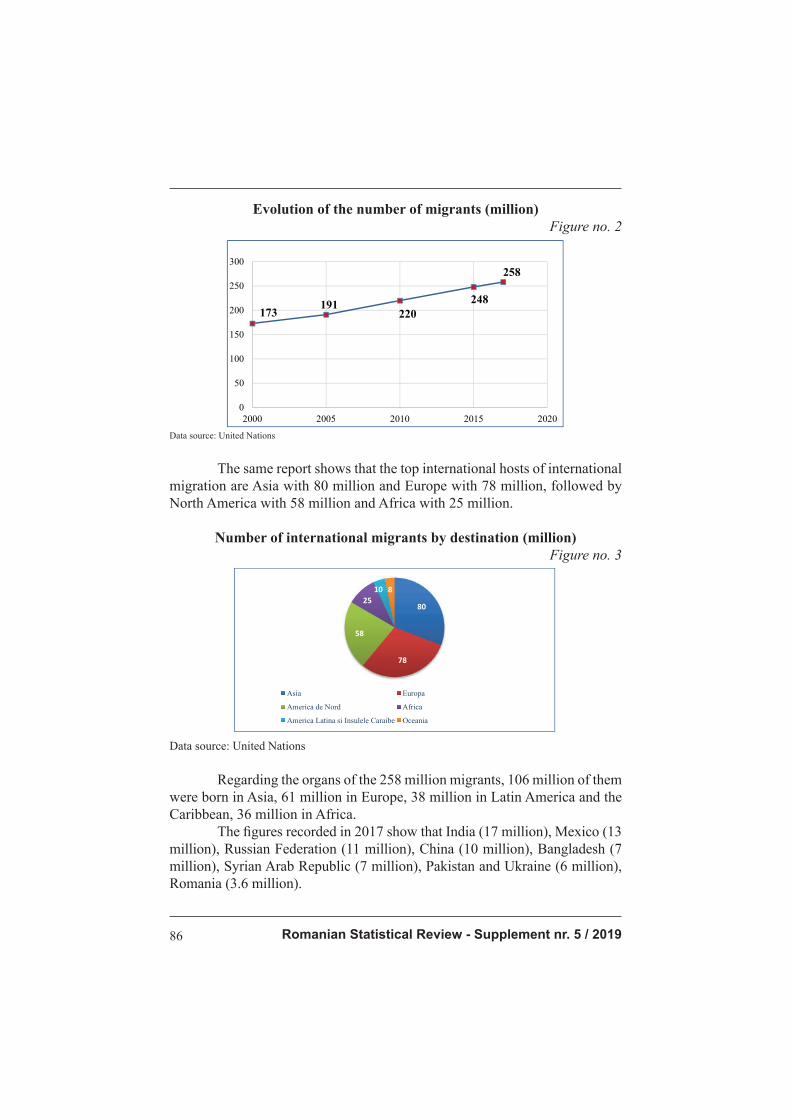
Romanian Statistical Review - Supplement nr. 5 / 201986
Evolution of the number of migrants (million)Figure no. 2
�
���� �������+������ 3���� 40� � �����4�����3��74�������8�
-69-;-
++5
+<=
+.=
)
D)
*))
*D)
())
(D)
;))
())) ())D ()*) ()*D ()()
Data source: United Nations
The same report shows that the top international hosts of international
migration are Asia with 80 million and Europe with 78 million, followed by
North America with 58 million and Africa with 25 million.
Number of international migrants by destination (million)Figure no. 3
�
���� �������9��� 40� ��4�����3�������%����3������,�� :0���$%���3���
��
��
��
��
�� �
%��� F� ��
%����������� �� %�����
%�������G���������C�����3����#� �������
Data source: United Nations
Regarding the organs of the 258 million migrants, 106 million of them
were born in Asia, 61 million in Europe, 38 million in Latin America and the
Caribbean, 36 million in Africa.
The fi gures recorded in 2017 show that India (17 million), Mexico (13
million), Russian Federation (11 million), China (10 million), Bangladesh (7
million), Syrian Arab Republic (7 million), Pakistan and Ukraine (6 million),
Romania (3.6 million).

Revista Română de Statistică - Supliment nr. 5 / 2019 87
In 2017, 67% of international migration was concentrated in 20
countries, the United States with 50 million international migrants ranks
among the countries of destination, the next being Saudi Arabia, Germany
and the Russian Federation, each hosting around 12 million migrants, England
and Northern Ireland, with about 9 million each.
Regarding the total number of refugees and asylum seekers, their
registered number was 25.9 million in 2016. Turkey (3.1 million), most of
which rank second and third in Jordan (2.9 million) and Palestine third (2.2
million).
The aim of this paper, however, is to analyze the impact of migrant
workers in countries of origin and destination. Refugees and asylum seekers
are therefore not part of this study and will not include determining the impact
of migration on the economic development of a country. We assume that the
main reason for migration is to improve the quality of life of the migrant as
well as of his family, the international migrant deserves the country of origin
from the desire to cover his needs such as: a better job, education, health. As
far as refugees and asylum seekers are concerned, they leave their countries
of origin mainly for political reasons. The large number of refugees in the
last two years, I do not think it should be included in this study because it is
a special case of migration, their integration into the countries of destination
requires time, and the contribution of these persons to the country’s economy
can be subsequently identifi ed after the integration of these social, economic
and fi nancial persons.
The tendency of international migrants is to move to developed
countries with high incomes, so there are 165 million international migrants
living in high-income countries globally.
The chart below shows the distribution of international migrants in high,
middle and low income countries. It is noticed that 64% of international
migrants choose high income countries, 32% of countries with average income
and only 4% are heading for low-income countries.
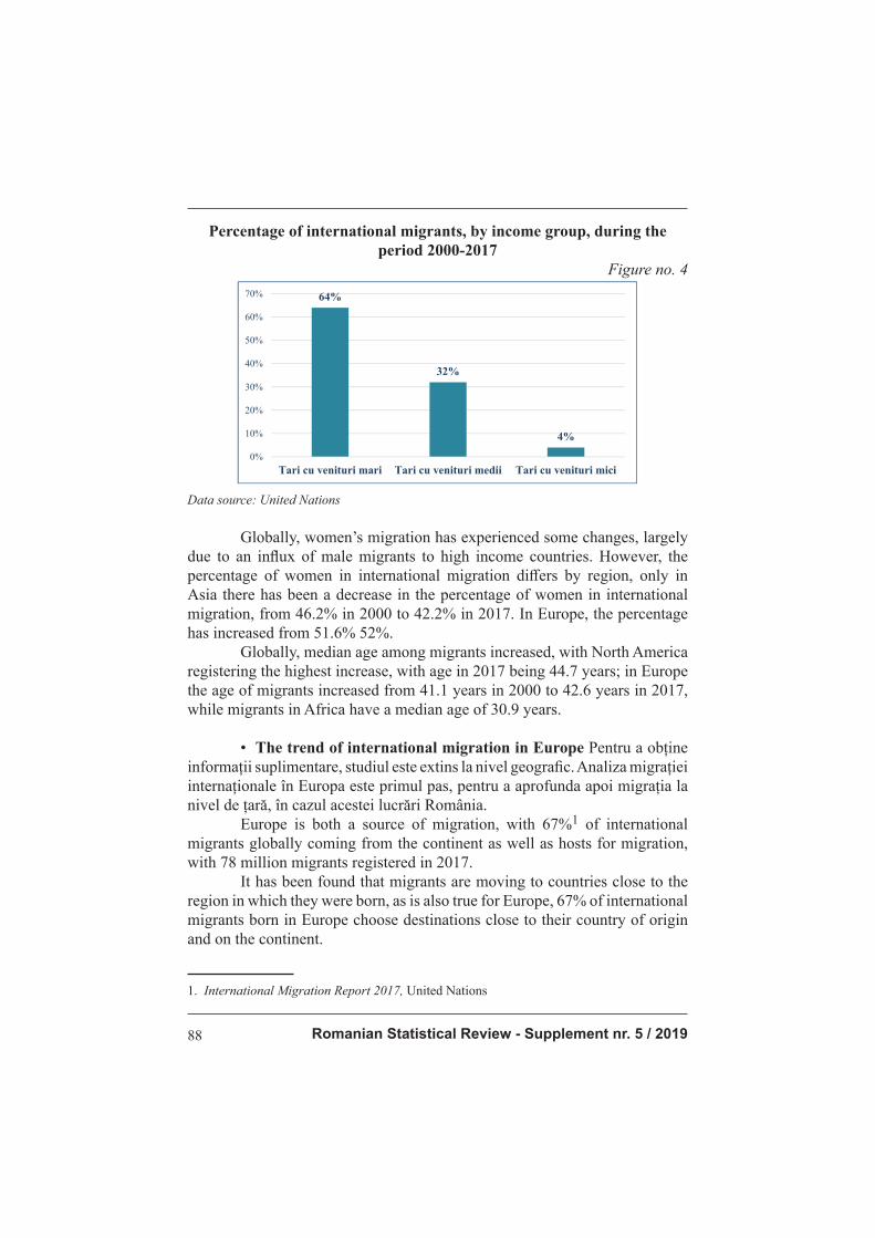
Romanian Statistical Review - Supplement nr. 5 / 201988
Percentage of international migrants, by income group, during the period 2000-2017
Figure no. 4
��� �������<��>��&��% ��4�����3�������%����3������,�:���� :���������% ��,�
A<B
9+B
<B
)I
*)I
()I
;)I
A)I
D)I
9)I
+)I
�����& �����% ���4��� �����& �����% ���4���� �����& �����% ���4�&�
Data source: United Nations
Globally, women’s migration has experienced some changes, largely
due to an infl ux of male migrants to high income countries. However, the
percentage of women in international migration diff ers by region, only in
Asia there has been a decrease in the percentage of women in international
migration, from 46.2% in 2000 to 42.2% in 2017. In Europe, the percentage
has increased from 51.6% 52%.
Globally, median age among migrants increased, with North America
registering the highest increase, with age in 2017 being 44.7 years; in Europe
the age of migrants increased from 41.1 years in 2000 to 42.6 years in 2017,
while migrants in Africa have a median age of 30.9 years.
• The trend of international migration in Europe Pentru a obține
informații suplimentare, studiul este extins la nivel geografi c. Analiza migrației
internaționale în Europa este primul pas, pentru a aprofunda apoi migrația la
nivel de țară, în cazul acestei lucrări România.
Europe is both a source of migration, with 67%1 of international
migrants globally coming from the continent as well as hosts for migration,
with 78 million migrants registered in 2017.
It has been found that migrants are moving to countries close to the
region in which they were born, as is also true for Europe, 67% of international
migrants born in Europe choose destinations close to their country of origin
and on the continent.
1. International Migration Report 2017, United Nations

Revista Română de Statistică - Supliment nr. 5 / 2019 89
At European Union (EU) level, according to Eurostat, by January 1,
2016, a total number of international migrants of 54.4 million people was
registered in the 28 member states. Of these, 35.1 million people came from
non-EU countries, and 19.3 million people were born in another EU country.
Figure no. 5 shows the 28 countries in the EU with the number of
migrants registered up to 2017. It can be seen that their number diff ers from
one country to another, it is preserved the global trend, that international
migrants choose to settle in developed countries , with high incomes. Thus,
12.5 million migrants were in Germany. Germany ranks fi rst in the EU,
followed by the UK (9.2 million), France (7.9 million), Spain (6.2 million)
and Italy (5.9 million).
Countries of destination for migrantsFigure no. 5
Source: World Bank, Bilateral Migration Matrix, data from 2017
On the other hand, there are EU countries such as: Romania, Bulgaria
or Poland, where the number of people moving to other countries exceeds the
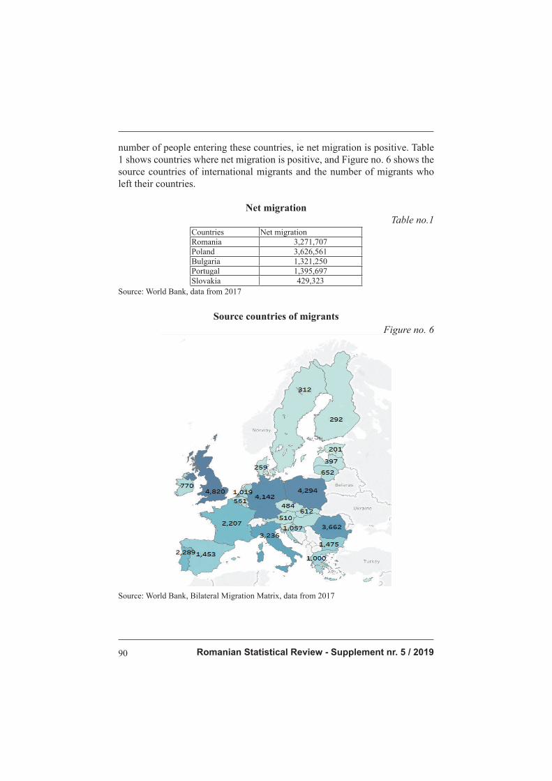
Romanian Statistical Review - Supplement nr. 5 / 201990
number of people entering these countries, ie net migration is positive. Table
1 shows countries where net migration is positive, and Figure no. 6 shows the
source countries of international migrants and the number of migrants who
left their countries.
Net migrationTable no.1
Countries Net migration
Romania 3,271,707
Poland 3,626,561
Bulgaria 1,321,250
Portugal 1,395,697
Slovakia 429,323
Source: World Bank, data from 2017
Source countries of migrantsFigure no. 6
Source: World Bank, Bilateral Migration Matrix, data from 2017
Revista Română de Statistică - Supliment nr. 5 / 2019 91
A series of statistical and econometric models are used in the
migration analysis. Asftel, the neoclassical model - macroeconomic approach
was originally developed to describe the impact of international migration
on economic development. The model hypotheses take into account the fact
that: international migration is determined by the wage diff erences between
the country of origin and the country of destination; it is assumed that the
elimination of these diff erences would lead to the cessation of international
migration; the diff erences between the infl ow of qualifi ed and unqualifi ed
human capital could result in a diff erent pattern of migration; the main
mechanism by which international labor fl ows are generated is the labor
market, other markets do not have the same impact as the labor market; how
governments control and infl uence the international labor market through
regulations both in the source and destination countries of migrants. The
neoclassical model - microeconomic approach represents a deepening of the
neoclassical macroeconomic model. The main assumption of the model is
that the migrant, ahead of his decision to leave his native country, looks very
well at the expected costs and income, cost-benefi t, social and technological conditions, and only when net expected earnings are higher than those in the native country choose to migrate.
Conclusion The most important consensus of the population movement, from the point of view of the economic activity of a country, is remittances. If the main reason the migrant chooses to leave his / her home country is to support his / her family and to cover his / her primary needs (food, house, clothing, etc.), he / she decides to send the family periodically a sum of money , so that these needs are met and family members’ quality of life improved. In many cases, the migrant chooses to transfer money to the family for health and support of children’s education. In the case of families with a volatile income, the decision is made that a family member is sent to another country to fi nancially support the household. Thus, the cost of migrating to another country is initially borne by the whole family in exchange for receiving a remittance income for a temporary period. Migrants can choose to leave their country of origin only to save income earned abroad, then to invest them either in the country of destination or in the country of origin. Thus, remittances sent by migrants are not used for consumption but are part of a long-term strategic behavior of the migrant, namely to make an investment. The decision to invest in the country of origin or the country of destination is infl uenced by factors
such as infl ation, macroeconomic stability, the environment or not to invest,
the need for investment in that market.

Romanian Statistical Review - Supplement nr. 5 / 201992
References 1. Anghel, M. G., Niță, G., Badiu, A. (2017). Impact of Remittances on Financial
Development and Economic Growth. Romanian Statistical Review Supplement, 1, 106-112
2. Anghelache, C., Niță, G., Badiu, A. (2017). Migration and remittances – statistical and econometric models used to analyze the impact of remittances in economic development. Romanian Statistical Review, Supplement, 6, 134-143
3. Anghelache, C. (2009). Statistical possibilities for the analysis of migration, Metalurgia Internaţional, XIV (14), Special Issue, 155-156
4. Artjoms I., King, R. (2012). Family Migration Capital and Migration Intentions. Journal of Family and Economic Issues, 33 (1), 118-129
5. Beets, G., Willekens, F. (2009). The global economic crisis and international migration: An uncertain outlook. Vienna Yearbook of Population Research, 19-37
6. Crowder, K., Hall, M., Tolnay, S. (2011). Neighborhood Immigration and Native Outmigration, American Sociological Review, 76 (1), 25-48
7. Giuliano, P., Ruiz-Arranz, M., (2009). Remittances, fi nancial development, and growth, Journal of Development Economics, 90, 144-152
8. Foley, M., Angjellari-Dajci, F. (2015). Net Migration Determinants. Journal of
Regional Analysis and Policy, 45 (1), 30-35 9. Kaplan, G., Schulhofer-Wohl, S. (2012). Interstate Migration Has Fallen Less
Than You Think: Consequences of Hot Deck Imputation in the Current Population Survey. Demography, Springer, 49 (3), August, 1061-1074
10. Kennan, J., Walker, J. R. (2011). The eff ect of expected income on individual
migration decisions. Econometrica, 79 (1), 211–251
11. Moreno-Galbisa, E., Tritah, A. (2016). The eff ects of immigration in frictional
labor markets: Theory and empirical evidence from EU countries. European
Economic Review, 84, 76–98
12. Zaiceva, A., Zimmermann, K.F. (2013). Returning Home at Times of Trouble?
Return Migration of EU Enlargement Migrants during the Crisis. Center for
Economic Research, Working Paper, 89, February
Revista Română de Statistică - Supliment nr. 5 / 2019 93
The Basel Agreements - The Analysis of the Banking Risks
Gabriela Victoria ANGHELACHE PhD ([email protected])
Bucharest University of Economic Studies, Romania
György BODÓ PhD Student ([email protected])
Bucharest University of Economic Studies
Radu STOICA PhD Student ([email protected])
Bucharest University of Economic Studies
Abstract The Basel Accords are the Basel Committee for Banking Supervision
(BCSB) regulations. It was established in 1974 with the Bank of International
Settlements (BIS). The name of the normative acts, the Basel Agreements,
drawn up by them, comes from the fact that these institutions are based in Basel
in Switzerland. BCSB aims to use the experience gained in banking activity
to understand the main factors governing this activity, to synthesize and to
harmonize good practice rules to reduce the risks associated with fi nancial-
banking activities and to improve the effi ciency of supervision banking.
The Committee proposes that its work should serve the purpose of
preventing, avoiding or at least limiting the eff ects of signifi cant crises. It
expresses its views through publications, exchange of information and
approaches on the promotion of banking supervision standards, but also
provides a common and coherent framework for the analysis of banking
supervision elements and their unitary treatment. The last big fi nancial
crisis in 2008 proved the usefulness of adopting the provisions of the Basel
Committee Agreement by most fi nancial and banking institutions. Even if in
many cases the recommendations were imposed by the banking supervisors in
the respective countries and were not adopted voluntarily, they have made their
eff ect, otherwise the eff ects of the crisis would have been more devastating.
Keywords: Basel, banking supervision, banking risk, fi nancial crisis
JEL Classifi cation: G21, G28
Introduction
Several versions of the recommendations with eff ects in the fi nancial
market have been developed over the past 30 years. The evolution and
complexity of the fi nancial and banking market as well as the global crisis
have led to the inclusion of new factors that have become signifi cant and have
led to continuous improvement of the recommendations. After the crisis, at
Romanian Statistical Review - Supplement nr. 5 / 201994
this time, a new version (now at the consultative level) known as BASEL IV
is being developed.
The Committee provides a common and coherent framework for
analyzing and dealing with the elements of banking supervision, and by
exchanging information, approaches and publications expresses its view on
the promotion of banking supervision standards, which are ultimately part of
a common vision aimed at preventing / avoiding signifi cant crises - or at least
limiting (restricting) their eff ects. As a comment on these issues, we can say
that the size of the last economic crisis would have been far more devastating
if most fi nancial and banking institutions did not implement the provisions
of the Basel Committee agreements - in many cases they were imposed by
banking supervisors from the respective countries.
Literature review Aebi, Sabato and Schmid (2012) analyzed a range of issues related to
risk management and bank performance in the context of the fi nancial crisis.
Anghelache, Sfetcu and Bodo (2017), as well as Anghelache, Anghel, Soare
and Badiu (2016), and Blum (2008) studied banking risks in the light of the
Basel agreements. Anghelache, Anghelache, Anghel, and Niţă (2016) presented
fundamental aspects of bank risks. Blundell-Wignall and Atkinson (2010)
highlighted the Basel III basics. Elsinger, Lehar and Summer (2006) treated
risk assessment for banking systems. Gasha et al. (2009) presented concepts of
credit risk modeling. Gordy and Howells (2006) examined aspects of the Basel
II agreement. Ippolito, Peydrób, Poloc and Sette (2016) presented elements of
liquidity risk management and Peters et al. (2009) of operational risk.
Methodology, data, results and discussions Over time, several versions of the recommendations have been
developed that have marked the fi nancial market for the last 30 years. The
banking fi nancial market has evolved a lot and has become increasingly
complex and diversifi ed, which has led to the inclusion of new factors
that have become signifi cant and the global crisis has led to the permanent
extension and improvement of the provisions. At this point, after the crisis, a
new version (still at the consultative level), which is known as BASEL IV, is
being developed.
• BASEL I Agreement It was the fi rst agreement and was developed in 1988 as the fi rst
BASEL agreement, which regulates the minimum capital requirements that
banks must have to deal with unforeseen situations that are considered as risk

Revista Română de Statistică - Supliment nr. 5 / 2019 95
events. This fi rst agreement envisaged three objectives: To ensure that banks
have suffi cient capital to cover their assumed risks; Facilitate comparison of
banks’ capital positions, which were greatly hampered by the use of diff erent
standards and calculation methods; To balance the conditions of competition
between international banks operating internationally. The need for the
agreement was determined by the fact that the conditions before the agreement
were very diff erent depending on the jurisdiction.
Basel I provided a fi rst coherent defi nition of eligible capital and
introduced risk factors that are weighted by the institutional nature of the
bank’s partners (mainly taking into account the exposure to credit risk but not
taking into account the intrinsic risks). The norm was revised in 1996, with the
inclusion of a new market risk component. On this occasion, and for the fi rst
time in Basel, banks were allowed to use internal risk assessment models.
• BASEL II Agreement This agreement was adopted in 2004 and introduced a series of
changes to the existing framework, which largely relied on the availability
of statistical data and models that allowed for more and more sophisticated
calculations but also the inclusion of new categories risk (operational risk,
market risk). The agreement introduces a structure of risk factors, which are
grouped on three pillars thus:
− Pillar 1: Minimum Capital Requirement - for the calculation of
the capital ratio, the credit risk was also included in the operational risk and
market risk.
− Pillar 2: Surveillance process - through which supervisors based
on their own assessments have the right to impose higher capital requirements
than Pillar 1 requirements, based on supervisory review.
− Pillar 3: market discipline - introduced the principles of
transparency and access to information on capital markets, requiring the
regular communication of risk-weighted capital.
In addition to these changes, the agreement also introduced a risk
treatment option (for Pillar 1) either in the Standard Approach (SD) based
on a set of predefi ned indices or on internal models based on Internal Ratings
Based (IRB) self-regulation validated by the supervisory authority. Also in the
agreement we meet for the fi rst time the obligation of banks to make stress-
test sensitivity simulations.
Under the BASEL II regulations we come across for the fi rst time
notions that have become commonplace both in the fi nancial and banking
market and in those related to risk rating systems.

Romanian Statistical Review - Supplement nr. 5 / 201996
PD = Probability of default of the creditor’s default;
LGD = Lost Given Default - loss due to non-payment;
EAD = Exposure at Default - risk exposure in case of non-payment;
EL = Expected Loss;
The relationship between the above is generically described by the
equation:
�� � �� � ��� � ���� � � � � �
The above indicators and their relationship are based on average
values (the principle of large numbers) under normal market conditions -
relative stability when variations caused by some participants are absorbed
by the system, but no longer meet the requirements in extraordinary situations
which may lead to a discontinuity of markets - crisis situations (eg excessive
growth, major / unilateral exposure, systemic risk, etc.).
The crisis that began in 2007 caught a signifi cant portion of banks
unprepared, although much of them had implemented BASEL II requirements.
This has led to the need to revise standards and to adopt much stricter
regulations in an attempt to anticipate or even prevent similar situations in the
future.
• BASEL III Agreement The drafting of the BASEL III agreement was generated by the
economic crisis that triggered a new wave of reforms that led to the adoption of
new rules in 2010. They set more stringent performance and prudential criteria
that would be able to absorb higher shocks absorption of losses), such as:
- Increase the minimum required capital level;
- Introduction of capital quality notion, defi ning diff erent capital
ranges, each having a specifi c coeffi cient;
- A non-risk lever (leverage factor) has been considered;
- The Liquidity Coverage Ratio (LCR) was introduced;
- Net Stable Funding Ratio (NSFR) was introduced.
In addition to the above, the regulations envisaged the adoption of
additional anti-cyclical capital buff ers that would function as an additional
absorption mechanism (shock absorber) of shocks of loss. The notion of
systemic risk has been introduced, which is related to capital add-on for
institutions that have a signifi cant role on the market, ie those that can induce
systemic risk - cascading problems from one bank to another that can generate
losses chain.
Another new approach is the diff erential treatment of banking (in
the classical sense) towards fi nancial (speculative) investment activities.
Thus, banks are required to manage diff erently the Banking Book and Asset
Portfolio respectively (Trading Book). The major diff erence between the two
Revista Română de Statistică - Supliment nr. 5 / 2019 97
approaches is refl ected (1) primarily in the nature of transactions - the former
refers to historical value when the transaction was recorded in the records and
the second to the expected market value at maturity, (2) and on the other hand
the risks associated with each of them - the fi rst is associated primarily with
credit risk, liquidity risk, interest rate, and the second on the risk of variation
of the share value, which depends on a lot of external and internal factors.
From the possibility of using the internal rating rates (IRBs) introduced
by BASEL II, some banks have implemented dedicated organizational
structures and developed a wealth of evaluation and simulation models to
enable them to optimize the Risk-Weighted Assets (RWA) risk index Assets)
- minimum capital for maximum exposure to risk. These calculations and
modeling are diffi cult to track and diffi cult to validate by external factors (such
as national or European supervisory structures), which has led to an inability
to compare institutions belonging to diff erent geographic regions or subject
to diff erent regulations. It has come to situations where, at an apparently
identical aggregate RWA level, institutions with profi les and very diff erent
risk exposures can actually be found.
The additional provisions introduced by BASEL III make it
increasingly diffi cult to apply the BASEL provisions and require an already
considerable increase in fi nancial institutions to meet these requirements.
Thus BASEL I, which was simple and transparent, reached BASEL III, which
is complicated and does not provide the expected transparency.
However, implementation of the provisions should have been
completed by the end of 2018, but at this point it is still too late to be able to
conclude if indeed all banks have aligned themselves with these provisions. In
parallel, ongoing analyzes are carried out, and hypotheses and proposals are
made to improve the situation - and predictability, in order to strengthen the
fi nancial-banking system so that the impact of a future crisis has a controllable
(as predictable) impact.
• Diffi culties encountered at the level of BASEL Agreements In turn, BASEL III is not so effi cient, though so elaborate, that with all
the diversifi cations and complications that may be involved, it can maintain
the stability of the world fi nancial banking system. Additional measures and
adjustments should be added to current ones to correct these shortcomings.
Opinions and ideas have already been published, with an advisory role, to
contribute to greater market stability. These initiatives take shape and are
marketed under the generic name of BASEL IV.
National / regional supervisory authorities have already taken steps to
tighten up capital requirements, increase prudential risk and reduce exposure
Romanian Statistical Review - Supplement nr. 5 / 201998
to high risk assets. Banks in turn have changed the balance sheet structure,
with a strong focus on increasing short-term liquidity. At the same time,
there is a tendency of banks to clear the loan portfolio (nonperforming), to
a considerable decrease in the appetite for lending, to the strengthening of
the capital position, to the attraction of deposits, all these tendencies led to a
signifi cant degradation of the their profi tability.
Decreasing profi tability is really a challenge for European banks given
the current context of low economic growth, negative interest rates, relative
stability in fi nancial markets. In addition, through the new restrictive measures,
the increase in regulatory pressure could further increase the competition gap
with US banks, which is why new measures are not a priority at this time
The new initiatives at work - still under debate - take into account the
following aspects:
- A new fundamental standard for the capital market (Trading
book), (given that the largest bankrupt banks were in the fi eld of investments -
capital markets). A fi rst variation has already been published and envisages an
increase in required capital (RWA) of at least 40%, and furthermore requires
complex and sophisticated tracking and obvious rules that will increase the
operational costs of business management and risk tracking ;
- The revised Banking Book Approach considers a more uniform
approach to specifi c risk assessment models based on indicators to be calculated
on the basis of information that no longer has a local or regional component ;
- The revision of credit methodologies - still in an early stage of
discussion - are considering a change in customer rating and assessment
(for example, a 3-fold increase is proposed for companies whose fi nancial
statements are not verifi ed);
- The review the impact on operational risk, which is estimated to
increase the impact on capital requirements by 40%. This is explained by an
increase in technological and processing processes and the vulnerability of the
human factor;
- The limiting the use of the Internal Evaluation Model (IRB)
approach, and increasing the overall index based approach to external factors -
the Standard Approach (SA). This is about reducing the use of internal methods
that did not provide an adequate degree of transparency and controllability
and the imposition of sector-specifi c minimum limits for each indicator. This
may lead to the need for a signifi cant increase in minimum capital for some
banking areas;
- The increase transparency on risk reporting, and use of similar indicators
and models - whether a bank is operating internationally or locally. This involves
a much higher data collection rate and adequate processing resources;

Revista Română de Statistică - Supliment nr. 5 / 2019 99
- The changing the approach to external rating agencies - these scores
will not be used directly to calculate the required capital, but will be taken into
account in market and customer valuation and pricing policies.
These proposals are in various stages of elaboration, debates,
discussions between specialists of specialized institutions, but no deadline has
yet been set for them to be adopted
Conclusion The new directives, although not yet fi nalized, have raised many
comments from stakeholders, who agree with the improvement of the
legal framework and on the other hand they want the proposals to focus on
minimizing the impact and not increasing signifi cant eff orts to implement the
proposed measures. The credit market is still at a considerably reduced level,
and new measures could lead to even greater reductions, perhaps even in the
few cases of blocking activity. An even greater reduction in lending could
have signifi cant negative eff ects on other branches of the economy, which
could lead to a new global crisis, this time an economic one.
References 1. Aebi, V., Sabato, G., Schmid, M. (2012). Risk management, corporate governance,
and bank performance in the fi nancial crisis. Journal of Banking and Finance, 36,
3213-3226
2. Anghelache, C., Sfetcu, M., Bodo, G. (2017). Analysis of Banking Risks in the Context
of The Basel Agreements. Romanian Statistical Review, Supplement, 12, 83-89
3. Anghelache, C., Anghel, M.G., Soare, D.V., Badiu, A. (2016). Banking Risk
evaluation Model based on BASEL Committee, International Symposium „Romania
in the European Union – Methods and Models of Macroeconomic Analysis and
Prognosis”, Bucharest, 19-20 may 2016, Editura Artifex, Bucureşti, 204-212 4. Anghelache, C., Anghelache, G.V., Anghel, M.G., Niţă, G. (2016). General Notions
on banking Risks. Romanian Statistical Review Supplement, 5, 13-18
5. Blum, J. (2008). Why ‘Basel II’ may need a leverage ratio restriction. Journal of
Banking & Finance, 32 (8), 1699-1707
6. Blundell-Wignall, A., Atkinson, P. (2010). Thinking beyond Basel III. Necessary
Solutions for Capital and Liquidity. OECD Journal Financial Market Trends, 2 (1), 9–33
7. Elsinger, H., Lehar, A., Summer, M. (2006). Risk Assessment for Banking Systems.
Management Science, 52 (9), 1301 - 1314
8. Gasha, J.G. et al. (2009). Recent Advances in Credit Risk Modeling, International
Monetary Fund in IMF Working Papers
9. Gordy, M., Howells, B. (2006). Procyclicality in Basel II: Can we treat the disease
without killing the patient?. Journal of Financial Intermediation, 15 (3), 395-417
10. Ippolito, F., Peydrób, J.L., Poloc, A. and Sette, E. (2016). Double bank runs and
liquidity risk management. Journal of Financial Economics, 122 (1), 135-154
11. Peters, G.W. et al. (2009). Dynamic Operational Risk: Modeling Dependence and
Combining Diff erent Sources of Information. The Journal of Operational Risk, 4
(2), 69-104
Romanian Statistical Review - Supplement nr. 5 / 2019100
Aspecte teoretice privind elaborarea previziunilor macroeconomice
Drd. Emilia STANCIU ([email protected])
Academia de Studii Economice din București
Drd. Marius POPOVICI ([email protected])
Academia de Studii Economice din București
Drd. Alexandra PETRE (OLTEANU) ([email protected])
Academia de Studii Economice din București
Drd. Andreea-Ioana MARINESCUAcademia de Studii Economice din București
Masterand Gabriela Iuliana CARAIANI ([email protected])
Universitatea „Artifex” din București
Daniel GHERASIM Master Student
Abstract Elaborarea cadrului metodologic al previzionării macroeconomice
presupune rezolvarea următoarelor trei mari probleme: structurarea
previziunilor; fundamentarea previziunilor: asigurarea unui fl ux logic al
lucrărilor de elaborare. Structurarea previziunilor înseamnă gruparea acestora,
a problemelor şi acţiunilor, după diverse criterii care să permită efectuarea
lucrărilor într-o asemenea ordine în raport cu competenţele celor care
elaborează astfel de lucrări şi care să asigure gradul dorit de operaţionalizare.
Prevederile previziunilor se structurează, însă, în mod diferenţiat pe: secţiuni
- grupe mari de probleme; profi luri - gruparea prevederilor după criteriul de
ramură, teritorial sau social; categorii de prevederi, respectiv orientative sau
imperative, priveşte în mod deosebit planurile şi programele. Fundamentarea
previziunilor macroeconomice înseamnă stabilirea fi ecăruia dintre elementele
acestora pe bază de informaţii sufi ciente, cu luarea în considerare a reţelei
de interdependenţe şi a evoluţiilor previzibile, asigurându-se, totodată, şi
măsuri de siguranţă asupra riscului şi incertitudini. Prin fundamentarea
previziunilor se urmăreşte desfăşurarea unor activităţi efi ciente din punct
de vedere tehnico - economic, social şi ecologic. Elaborarea lucrărilor de
previzionare macroeconomică presupune parcurgerea a trei etape esenţiale,
şi anume: diagnoza, prognozarea şi planifi carea sau programarea. Toate
acestea se afl ă în raporturi informaţionale şi de condiţionare metodologică.
Cuvinte cheie: diagnoză, prognozare, planifi care, metodă, previziune
macroeconomică
Clasifi carea JEL: C40, G17
Revista Română de Statistică - Supliment nr. 5 / 2019 101
Introducere Orice lucrare previzională este precedată de efectuarea unor analize complexe cu caracter retrospectiv, care să pună în evidenţă desfăşurarea activităţilor economico-sociale în perioada precedentă, tendinţele manifestate până la începutul perioadei care face obiectul previziunii. Acest demers poartă numele de analiză diagnostic sau diagnoză şi prezintă o situaţie sugestivă asupra nivelului de dezvoltare atins şi a factorilor care au condiţionat evoluţiile evidenţiate. Elaborarea prognozelor trebuie să parcurgă următoarele etape: interpretarea şi valorifi carea informaţiilor furnizate de analiza-diagnostic, precum şi a altor informaţii disponibile; elaborarea studiilor prospective şi a prognozelor preliminare; elaborarea prognozei macroeconomice preliminare; elaborarea prognozelor parţiale sau sectoriale, altele decât cele prioritare; elaborarea prognozei macroeconomice fi nale sau defi nitive.
Literature review Anghelache, Mitruţ și Voineagu (2013) au analizat principalele noțiuni teoretice și practice utilizate în analiza macroeconomică. Anghelache, Anghel, Jweida, Popovici și Stanciu (2016) au studiat aspecte ale estimării statistice. Anghelache (2008) tratează elementele fundamentale ale statisticii economice. Benjamin, Herrard, Houée-Bigot și Tavéra (2010) au studiat utilizarea modelelor econometrice în previziune. Carroll (2003) a analizat aspecte ale previziunii gospodăriilor. Clark și Ravazzolo (2015) au cercetat caracteristici ale performanței macroeconomice. Eckela, Philip și Grossman (2008) au examinat atitudini ale riscului în activitatea de previziune. Lucas, R.E. Jr. (2003) a cercetat prioritățile macroeconomice. Pesaran, Pick și Pranovich (2013), precum și Wilms și Croux (2016) au analizat elemente de bază ale activității de previzionare.
Metodologia cercetării, date, rezultate și discuții
Prognozele prioritare se elaborează pe baza concluziilor desprinse din analiza diagnostic şi din studiile prospective. Acestea se referă la domenii sau probleme care prezintă un interes deosebit pentru evoluţia economico-socială, dar care pot fi abordate relativ autonom, înainte de proiectarea structurilor macroeconomice, de ansamblu. Pe baza ansamblului de informaţii furnizate de lucrările previzionale menţionate se elaborează prognoza macroeconomică preliminară, ca model agregat coerent al evoluţiei economiei naţionale, prezentat într-o formă simplifi cată. Prognozele parţiale sau sectoriale au caracter complex dar relativ dezagregat. Se elaborează pe baza informaţiilor furnizate de studiile de
Romanian Statistical Review - Supplement nr. 5 / 2019102
analiză-diagnostic la nivel macroeconomic sau pe domeniile care constituie obiectul lor, de studiile prospective specifi ce şi de prognozele prioritare. Programele sau planurile macroeconomice şi sectoriale se elaborează de către ministerele sau departamentele interesate în colaborarea cu instituţii specializate publice sau private. Elaborarea planurilor şi programelor macroeconomice prezintă o serie de particularităţi şi în funcţie de orizontul de timp pe care îl iau în consideraţie şi anume: termen lung, peste 7 ani, pentru planuri sau programe strategice; termen mediu, cuprins între 3 şi 7 ani; planuri sau programe anuale. Metoda previzională este un mod de cercetare şi cunoaştere a realităţii pentru a anticipa o acţiune viitoare pe baza unor criterii de raţionalitate, de optim şi reprezintă o componentă a procesului de cunoaştere, arătând calea (căile) de urmat, ca rod al transformării enunţului teoretic privind dinamica economică în modalităţi şi procedee practice asupra felului cum trebuie procedat. Ansamblul metodelor folosite în domeniul previziunii, integrate într-o concepţie generală unitară, constituie metodologia previzională. Ţinând seama de practica planifi cării şi prognozării economico-sociale, metodele previzionale folosite pot fi : fundamentale; de previziune pe elemente; structurale, de stabilire în perspectivă a unor sisteme informatice; intuitive şi de echilibrare. Analiza constă în descompunerea fenomenului sau procesului respectiv în elementele sale constitutive, în scopul studierii aprofundate a acestora. Sinteza constă în recompunerea întregului din elementele analizate, obţinându-se expresii cantitative agregate şi generalizarea aspectelor particulare ale realităţii, în urma procesului de cunoaştere de la simplu la complex. Sintezele economico-sociale sunt instrumente indispensabile ale managementului şi previziunilor macroeconomice, constituind premisa necesară a exprimării opţiunilor şi adaptării deciziilor de importanţă naţională. În cadrul analizei (interpretării) sistemice, activitatea previzională presupune o serie de obiective, dintre care amintim: proiectarea indicilor de performanţă pentru starea dorită pe traiectoria dintre perioada de bază şi orizontul previziunii; stabilirea algoritmilor de determinare a variantelor convenabile; introducerea în sistem a variabilelor de intrare şi a parametrilor de decizie, precum şi obţinerea variabilelor de ieşire, cu luarea în considerare a fl uxurilor intermediare şi optimizarea funcţionării sistemului (a variantelor formulate).
Revista Română de Statistică - Supliment nr. 5 / 2019 103
• Metoda extrapolării Extrapolarea constă, în esenţă, în prelungirea în viitor a evoluţiei constatate în trecut. În raport de datele disponibile şi de specifi cul problemei analizate se utilizează diferite procedee de extrapolare şi anume extrapolarea analitică, extrapolarea fenomenologică, extrapolarea prin curbă înfăşurătoare. Extrapolarea analitică porneşte de la ipoteza unei evoluţii ai cărei parametrii se determină astfel încât să se obţină cele mai mici erori de estimare. Aceasta se poate aplica unor serii cronologice sau unei funcţii de corelaţie. Extrapolarea analitică cu ajutorul seriilor cronologice presupune determinarea trendului unei variabile după ce variaţia sezonieră a fost eliminată (printr-o metodă oarecare) sau dacă nu este afectată de variaţia sezonieră. Extrapolarea de acest gen se poate realiza, în problemele simple, cu ajutorul sporului mediu (absolut), cu alte cuvinte a raţiei medii, sau cu ajutorul ritmului mediu anual. Extrapolarea cu ajutorul sporului mediu (absolut) anual, adică a raţiei medii calculată cu ajutorul seriei dinamice statistice. În cazul extrapolării mecanice, se determină mai întâi sporurile cu baza în lanţ (pentru fenomenele care au tendinţa de evoluţie sub forma unei progresii aritmetice) şi apoi se stabileşte sporul mediu. Pentru extrapolare se foloseşte relaţia:
unde: = variabila extrapolată pentru orizontul “t” al previziunii;
= valoarea variabilei în anul de bază; = numărul de ani de după cel de bază până la orizontul “t” al previziunii; = sporul mediu anual.
În cazul unei extrapolări euristice se modifi că parametrul Δy, devenind Δy*, cu ajutorul produsului dintre sporul mediu şi coefi cientul k, ce poate fi mai mare sau mai mic decât l, după cum estimează specialiştii că se va modifi ca tendinţa evoluţiei. Dacă k<1 se reduce sporul mediu calculat pe baza datelor din perioada expirată, iar dacă k>l acest spor se amplifi că. Deci se aplică relaţia:
Extrapolarea cu ajutorul ritmului mediu anual, presupune mai întâi, determinarea indicilor de evoluţie cu baza în lanţ şi calcularea indicelui mediu
Romanian Statistical Review - Supplement nr. 5 / 2019104
al evoluţiei (pentru fenomenele care au tendinţa de a evolua sub forma unei progresii geometrice). Pentru extrapolarea mecanică se foloseşte relaţia:
unde: r = ritmul mediu anual al sporului, sub formă de indice; t = numărul de ani de după cel de bază, până la orizontul previziunii (ceilalţi termeni au aceeaşi semnifi caţie ca mai sus). În cazul unei extrapolări euristice se poate utiliza coefi cientul „k”, adică: În cazul problemelor mai complexe se procedează la alegerea tipului de funcţie (dreaptă, parabolă etc.) care să ajusteze cel mai bine datele seriei. Extrapolarea analitică cu ajutorul funcţiei de corelaţie constă în proiectarea variabilei dependente „Y” în corelaţie cu evoluţia variabilei independente „x”: Y=f(x)
Este obligatoriu însă ca între cele două variabile să existe relaţii cauzale, iar coefi cientul de corelaţie dintre ele să fi e cât mai mare şi abaterea medie pătratică să fi e cât mai mică. Aceste cerinţe trebuie urmărite când se alege forma funcţiei (sau se alege acea funcţie care satisface cel mai complet aceste exigenţe). Extrapolarea de acest tip pleacă de la ipoteza că oricare din valorile reale ale seriei dinamice se obţin prin suprapunerea următoarelor elemente: o variaţie stabilă de lungă durată, numită tendinţă, care dă sensul general al evoluţiei; variaţii periodice în jurul acestei tendinţe; variaţii întâmplătoare (aleatoare). În acest caz, relaţia de mai sus devine: Y = f(x) + u
unde: u = variabila aleatoare (perturbatoare)
Succesiunea calculelor pentru realizarea unei extrapolări analitice bazate pe funcţii de corelaţie este următoarea: stabilirea mărimilor (variabilelor) de previziune pentru care se analizează corelaţia, cu condiţia ca între ele să existe o dependenţă reală. În caz că se foloseşte o corelaţie multiplă se va urmări ca între variabilele independente să nu existe o infl uenţă reciprocă
(să nu fi e autocorelate); alegerea perioadei statistice pentru care şirurile de date disponibile sunt concludente; reprezentarea grafi că a şirurilor de date statistice, obţinându-se în acest fel o primă indicaţie asupra formei funcţiei ce
Revista Română de Statistică - Supliment nr. 5 / 2019 105
poate fi utilizată; verifi carea ipotezei cu privire la forma funcţiei; determinarea
parametrilor funcţiei, de regulă, prin metoda celor mai mici pătrate; calculul
estimatorilor statistici, pentru a stabili intensitatea legăturii; determinarea prin
extrapolare a mărimii variabilei dependente pentru anul de prognoză sau de
plan/program şi analiza critică a rezultatelor obţinute, care se compară cu cele
dobândite prin alte metode.
Extrapolarea fenomenologică constă în analiza caracteristicilor
globale ale fenomenului, pe baza interpretării logice a experienţei practice
de durată. Se pot desprinde astfel anumite „legi” de variaţie a fenomenului
urmărit, în condiţiile date. Metoda se bazează pe reprezentarea grafi că,
evidenţiindu-se vizual tendinţele de evoluţie. Rezultanta poate fi o dreaptă
exprimată ca o funcţie liniară simplă (Xt = a + by), iar pentru evoluţii mai
complexe curbele pot fi descrise de funcţii exponenţiale, logaritmice, logistice
etc.
Extrapolarea prin curbe înfăşurătoare descrie dinamica rezultantei
unor procese complexe, formate din mai multe elemente care intervin succesiv
în evoluţia de ansamblu a procesului. Cu alte cuvinte, ea constă în ajustarea
(înfăşurarea) unei serii de curbe secvenţiale.
• Metoda interpolării Metoda interpolării constă în stabilirea mărimilor intermediare între
două variabile date, şi anume între nivelul anului de bază şi cel prevăzut pentru
anul fi nal al perioadei de prognoză sau de plan.
Interpolarea se poate realiza folosind două procedee:
- interpolarea cu ajutorul raţiei medii anuale stabilită în funcţie de cele
două mărimi cunoscute (X0 şi XT) şi de numărul de ani dintre ele:
R=(X, - Xo)/T
X�=X �+(R -T )
unde:
R = raţia medie anuală;
XT = nivelul variabilei exogene pentru anul fi nal T;
X0 = nivelul variabilei din anul de bază;
T = numărul de ani dintre anul de bază şi anul fi nal;
Xt = nivelul variabilei rezultative, interpolate, pentru un an oarecare t,
situat între anul de bază şi cel fi nal;
t = numărul de ani dintre anul de bază şi anul „t”
- interpolarea cu ajutorul ritmurilor medii, stabilindu-se
ritmul mediu anual dintre anul de bază şi cel fi nal al previziunii şi aplicându-l
din aproape în aproape la valorile absolute intermediare. Se folosesc relaţiile:
Romanian Statistical Review - Supplement nr. 5 / 2019106
De unde:
și:
de unde:
unde:
r = ritmul mediu anual al sporului;
XT = nivelul anului fi nal;
X0 = nivelul anului de bază;
n = numărul de ani dintre „0” şi „t”; „t” = un an oarecare dintre „0” şi „T”.
• Modele utilizate în elaborarea prognozelor Dacă vom considera că există parametri constanţi pe perioada prognozei, vom observa că modelul autoregresiv este greșit specificat, în
comparaţie cu un model corect specificat de tip corecţia echilibrului. Ca atare,
prognoza primului model va fi mai slabă. Dar, dacă parametrii se schimbă
după ce se face prognoza, cel de-al doilea model va fi și el expus, fiind greșit
specificat pe perioada prognozei. Pe de altă parte, orice model autoregresiv
poate fi privit ca un caz special al modelului de corecţie, justificare fiind că
impunere stricții de rădăcina unitară adiţională în cadrul sistemului. Schimbarea
în perioada prognozei a parametrilor asociaţi variabilelor de nivel excluse din
modelul dVAR conduce la specifi carea eronată a modelului EqCM. Astfel,
factorul determinant este mecanismul de generare care predomină.
Discontinuităţile structurale se manifestă diferit asupra celor două tipuri
de modele, în erorile de prognoză. Avem în vedere că modelele de prognoză
practice sunt sisteme deschise, cu variabile exogene. Proprietăţile modelelor
studiate sunt utile în interpretarea erorilor de prognoză ale sistemelor mari.
Revista Română de Statistică - Supliment nr. 5 / 2019 107
Pentru cei care realizează prognoze, este relevantă tendinţa deterministă liniară pentru mai multe variabile de interes. Ca exemple, putem menţiona indicatorii cererii si preţurilor externe si productivitatea medie a muncii. Prin poziţie, alte variabile ca de exemplu preţurile petrolului si instrumentele de politică monetară, adică ratele dobânzii si cursurile de schimb sunt mai apropiate de ipoteza de tendinţă zero. Este importantă reprezentarea impactului modificărilor de parametri asupra prognozelor efectuate prin cele două modele.
• Previzionarea relatiilor economice externe Sfera de activitate a relaţiilor economice externe cuprinde: comerţul exterior propriu-zis; comerţul exterior invizibil; servicii; cooperarea economică şi tehnico-ştiinţifi că internaţională în domeniul producţiei industriale, agricole,
al activităţii de construcţii, transporturi, comerţ, cercetare tehnico-ştiinţifi că,
servicii, operaţiuni bancare.
Procesele au loc între unităţi aparţinând unor economii naţionale
diferite, chiar dacă în unele cazuri exportul nu depăşeşte frontierele naţionale
ale furnizorului, cum se întâmplă cu vânzările de bunuri şi servicii prestate
turiştilor străini pe teritoriul naţional.
Activitatea de previziune cuprinde: activitatea de prospectare-
prognozare; activitatea tranzacţională; activitatea de elaborare a previziunilor
pe termen scurt privind relaţiile economice externe.
- Modele economico-matematice utilizate în prognozarea relaţiilor
economice externe
Funcţiile de corelaţie
- evoluţia exportului total (Mt) ca funcţie de evoluţie a venitului
naţional creat sau P.I.B.
M t = f(V)
- evoluţia exportului, folosindu-se ponderea acestuia în volumul
venitului naţional creat sau al P.I.B. (Kmt) ca funcţie de trend stabilită opţional:
M t = Vt x Kmt
- evoluţia exportului pe ramuri şi subramuri cu aceleaşi funcţii, dar
utilizându-se indicatori pe ramuri;
- evoluţia exportului pe subramuri, grupe de produse şi produse
principale cu ajutorul unor indici normativi: export la un milion lei producţie
marfă; export la un milion tone cereale; export de maşini, aparate, mijloace de
transport la 1000 bucăţi produse etc.;
- evoluţia importului total (Nt) ca funcţie de evoluţie a P.N.B. (Pt)
având în vedere că importul este implicat atât în producţia intermediară, cât şi
în crearea produsului fi nal:
Romanian Statistical Review - Supplement nr. 5 / 2019108
N t = f (Pt)
- evoluţia importului cu ajutorul coefi cientului importului în volumul
P.N.B. (Knt) ca funcţie de trend stabilite opţional:
N t = Pt x K„t.
Modelul matriceal (de reţea) relevă curenţii de mărfuri şi servicii ale
unei ţări cu exteriorul; poate fi reprezentat sintetic astfel:
unde:
= coefi cientul caracteristic al țării importatoare „j” în perioada
de previziune;
= volumul X al curenților de mărfuri și servicii din țara de origine
„i” spre țara „j” în anul de previziune t;
= volumul acelorași curenți în anul de bază t0;
= coefi cientul caracteristic al țării exportatoare „i” în perioada de
previziune.
Modelul gravitaţional este conceput prin luarea în calcul a gradului
de dezvoltare economică şi a distanţei economice dintre parteneri, din punct
de vedere al ţării exportatoare. Expresia generalizată a modelului gravitaţional
este următoarea:
unde:
Xij = volumul X al curenților de mărfuri și servicii din țara exportatoare
„i” către țara importatoare „j”;
Vi = venitul național pe locuitor al țării exportatoare „i”;
Vj = venitul național pe locuitor al țării importatoare „j”;
kij = coefi cientul care exprimă distanța economică dintre parteneri;
α = elasticitatea exportului țării „i” în raport cu propriul venit național
pe locuitor;
β = elasticitatea importului țării „j” în raport cu propriul venit național
pe locuitor.
Cu ajutorul previziunii se prestabilește, prin metode și mijloace
specifi ce, componența, dinamica și efi ciența unor acțiuni ce urmează să
aibă loc. Prefi gurarea este o schițare în linii mari a ceea ce urmează să se
întâmple, ea se face de obicei în primele faze când se stabilesc liniile mari de
Revista Română de Statistică - Supliment nr. 5 / 2019 109
acțiune, tendința. Predeterminarea este o previziune mai complexă, în cadrul ei sunt luate în calcul, prin tehnici variate, mai multe variante, se analizează maximizarea outcome-ului și se minimizează riscurile, în consecință sunt cântărite soluțiile optime. Toate varintele de previziuni: prognoze, strategii, planuri, programe, etc trebuie să combine elementele deterministe cu cele aleatoare, întrucât viitorul este deopotrivă condiționat de necesitate dar este și întâmplare.
Concluzii Tehnicile cantitative pot măsura elementele deterministe, adică cele cauzate prin relația cauză-efect dar nu pot identifi ca elementele aleatoare. Elementele deterministe sunt acele cauze care în decursul timpului au avut aceleați efecte, pe când elementele aleatoare, fi e au avut loc în trecut dar sporadic, fi e sunt riscuri imprevizibile ce pot apărea oricând în prezent sau în viitor. Se identifi că din acest punct de vedere mai multe categorii de previziuni: previziuni în condiții de risc, previziuni în condiții de incertitudine, previziuni în condiții de ambiguitate. În cazul previziunilor în condiții de risc, este anticipat nivelul de risc și posibilele tipuri de rezultate, dar nu se poate anticipa măsura în care are loc un rezultat. În situațiile simple de acest caz, sunt luate decizii cu risc minim, iar în cazurile mai complexe se iau decizii cu raport corect între riscul posibil și costul anti-riscului. În cazul previziunilor în condiții de incertitudine, nu sunt cunoscute nici rezultatele, nici gradul lor de realizare. În aceste cazuri, sunt folosite și alte informații pentru a se determina marja de producere a anumitor rezultate. În situația previziunilor în condiții de ambiguitate, incertitudinea este cauzată de date irelevante ce ingreunează sau fac imposibilă estimarea probabilității de producere a unui fenomen.
Bibliografi e
1. Anghelache, C., Mitruţ, C., Voineagu, V. (2013). Statistică macroeconomică:
sistemul conturilor naţionale. Editura Economică, Bucureşti 2. Anghelache, C., Anghel, M.G., Jweida, I.J., Popovici, M. and Stanciu, E. (2016).
Theoretical notions of statistical estimation. Romanian Statistical Review
Supplement, 11, 120-126 3. Anghelache, C. (2008). Tratat de statistică teoretică şi economică, București:
Editura Economică 4. Benjamin, C., Herrard, N., Houée-Bigot, M., Tavéra, C. (2010). Forecasting with
an Econometric Model, Springer 5. Carroll, Ch. (2003). Macroeconomic Expectations of Households and Professional
Forecasters. Quarterly Journal of Economics, 118 (1), 269-298 6. Clark, T., Ravazzolo, F. (2015). Macroeconomic Forecasting Performance
under Alternative Specifi cations of Time-Varying Volatility. Journal of Applied
Econometrics, 30 (4), 551–575
Romanian Statistical Review - Supplement nr. 5 / 2019110
7. Eckela, C., Philip J., Grossman, P. (2008). Forecasting risk attitudes: An
experimental study using actual and forecast gamble choices. Journal of Economic
Behavior & Organization, 68 (1), 1–17
8. Lucas, R.E. Jr. (2003). Macroeconomic Priorities. American Economic Review, 93
(1), 1-14
9. Pesaran, H., Pick, A., Pranovich, M. (2013). Optimal forecasts in the presence of
structural breaks. Journal of Econometrics, 177 (2), 134-152
10. Wilms, I., Croux, C. (2016). Forecasting using sparse cointegration. International
Journal of Forecasting. 32 (4), October–December 2016, 1256–1267.
Revista Română de Statistică - Supliment nr. 5 / 2019 111
THEORETICAL ASPECTS REGARDING THE ELABORATION OF THE MACROECONOMIC
FORECASTS
Emilia STANCIU PhD Student ([email protected])
Bucharest University of Economic Studies
Marius POPOVICI PhD Student ([email protected])
Bucharest University of Economic Studies
Alexandra PETRE (OLTEANU) PhD Student ([email protected])
Bucharest University of Economic Studies
Andreea-Ioana MARINESCU PhD StudentBucharest University of Economic Studies
Gabriela Iuliana CARAIANI Master Student ([email protected])
„Artifex” University of Bucharest
Daniel GHERASIM Master Student
Abstract The elaboration of the methodological framework of the
macroeconomic forecast involves solving the following three major problems:
structuring the forecasts; substantiating forecasts: ensuring a logical fl ow
of drafting work. Structuring the forecasts means grouping them, problems
and actions, according to various criteria that allow the work to be done
in such order in relation to the skills of those who develop such works and
to ensure the desired degree of operationalization. The provisions of the
forecasts are structured, however, in a diff erentiated way on: sections - large
groups of problems; profi les - grouping provisions by branch, territorial or
social criterion; categories of provisions, namely indicative or imperative,
are particularly relevant to plans and programs. Establishing macroeconomic
forecasts means setting each of their elements on the basis of suffi cient
information, taking into account the network of interdependencies and
predictable developments, while ensuring risk and uncertainty measures.
The substantiation of the forecasts is aimed at carrying out activities that are
technically, economically, socially and ecologically effi cient. The elaboration
of the macroeconomic forecasting projects involves the following three
essential steps, namely: diagnosis, forecasting and planning or programming.
All of this is in information and methodological conditioning.
Keywords: diagnosis, prognosis, planning, method, macroeconomic
forecast
JEL classifi cation: C40, G17
Romanian Statistical Review - Supplement nr. 5 / 2019112
Introduction Any predictive work is preceded by complex retrospective analyzes,
which show the development of economic and social activities in the previous
period, the trends manifested up to the beginning of the period underlying
the forecast. This is called Diagnostic or Diagnostic Analysis and presents a
suggestive situation on the level of development reached and the factors that
have conditioned the evolved developments.
Elaboration of forecasts should follow the following steps:
interpretation and capitalization of the information provided by the diagnostic
analysis, as well as other available information; development of prospective
studies and preliminary forecasts; preparing the preliminary macroeconomic
forecast; the development of partial or sectoral forecasts other than priority
ones; preparing the fi nal or fi nal macroeconomic forecast.
Literature review Anghelache, Mitruţ and Voineagu (2013) analyzed the main
theoretical and practical notions used in the macroeconomic analysis.
Anghelache, Anghel, Jweida, Popovici and Stanciu (2016) studied aspects
of statistical estimation. Anghelache (2008) deals with the fundamentals
of economic statistics. Benjamin, Herrard, Houee-Bigot and Tavéra (2010)
studied the use of econometric models in the forecast. Carroll (2003)
analyzed aspects of the households’ forecast. Clark and Ravazzolo (2015)
investigated features of macroeconomic performance. Eckela, Philip and
Grossman (2008) examined risk attitudes in predictive activity. Lucas,
R.E. Jr. (2003) investigated macroeconomic priorities. Pesaran, Pick and
Pranovich (2013), and Wilms and Croux (2016) analyzed basic elements of
predictive activity.
Research methodology, data, results and discussions The priority prognoses are based on the fi ndings of the diagnostic
and prospective studies. These relate to areas or issues of particular interest to
socio-economic development but can be approached relatively autonomously
before designing macroeconomic structures as a whole.
On the basis of the information provided by the forecasted works, the
preliminary macroeconomic forecast is developed as a coherent aggregated
model of the evolution of the national economy presented in a simplifi ed
form. Partial or sectoral projections are complex but relatively disaggregated.
It is elaborated on the basis of the information provided by macroeconomic
analysis-diagnosis studies or the areas that are their subject, specifi c prospective
studies and priority forecasts.
Revista Română de Statistică - Supliment nr. 5 / 2019 113
Macroeconomic and sectoral programs or plans are developed by
interested ministries or departments in collaboration with public or private
specialized institutions. The elaboration of the macroeconomic plans and
programs presents a number of peculiarities and according to the time
horizon that they take into account, namely: over 7 years for strategic plans or
programs; medium term, ranging from 3 to 7 years; plans or annual programs.
The predictive method is a mode of research and knowledge of
reality to anticipate future action based on rationality, optimal criteria, and
is a component of the knowledge process, showing the way (s) to follow as
the fruit of transforming the theoretical statement on economic dynamics in
practical ways and procedures on how to proceed.
The set of methods used in the fi eld of forecasting, integrated into a
unitary general concept, is the predictive methodology.
Taking into account the practice of economic and social forecasting
and forecasting, the predictive methods used can be: fundamental; prediction
on items; structural, forward-looking computer systems; intuitive and
balancing.
The analysis consists in the decomposition of the respective
phenomenon or process into its constitutive elements for the purpose of their
in-depth study.
The synthesis consists in recomposing the whole of the analyzed
elements, generating aggregate quantitative expressions and generalizing
the particular aspects of reality, following the process of knowing from
simple to complex. Economic and social syntheses are indispensable tools of
macroeconomic management and forecasting, being the prerequisite for the
expression of options and the adaptation of decisions of national importance.
In the systemic analysis, the predictive activity involves a series of
objectives, among which: designing the performance indices for the desired
state on the trajectory between the base period and the forecast horizon;
establishing algorithms for determining the appropriate variants; introducing
input variables and decision parameters into the system, as well as obtaining
output variables, taking into account the intermediate fl ows and optimizing
system operation (of the formulated variants).
• Extrapolation method Extrapolation consists essentially in the future extension of past
developments.
In relation to the available data and the specifi city of the analyzed
problem, diff erent extrapolation methods are used, ie analytical extrapolation,
phenomenological extrapolation, extrapolating by wrapping curve.

Romanian Statistical Review - Supplement nr. 5 / 2019114
Analytical extrapolation starts from the hypothesis of an evolution
whose parameters are determined so as to obtain the smallest estimation
errors. This may apply to chronological series or to a correlation function.
Analytical extrapolation using chronological series involves determining the
trend of a variable after the seasonal variation has been eliminated (by some
method) or if it is not aff ected by the seasonal variation. Extrapolation of this
kind can be achieved in simple issues with average (absolute) growth, in other
words the average ration, or with the average annual rate.
Extrapolation with average (absolute) annual growth, ie average
ration calculated using the dynamic statistical series. In the case of mechanical
extrapolation, the chain-based increases are fi rst determined (for phenomena
that tend to evolve in the form of an arithmetic progression) and then the
average increase is determined. For extrapolation use the relationship:
where:
= the extrapolated variable for the „t” horizon of the forecast;
= the value of the variable in the base year;
= number of years after the base year up to the horizon „t” of the
forecast;
= annual average growth.
In case of a heuristic extrapolation, the parameter Δy changes to Δy*,
with the product of the average increase and the coeffi cient k, which may be
higher or lower than l, as the experts estimate that the evolution trend will
change. If k <1 reduces the average gain calculated based on expired date
data, and if k> l this gain is amplifi ed. So the relationship applies:
The extrapolation with the average annual rhythm presupposes, fi rstly,
the determination of the chain-based evolution indices and the calculation of
the average evolution index (for phenomena that tend to evolve in the form
of a geometric progression). For mechanical extrapolation the following
relationship is used:
where:
r = average annual growth rate in index form;
t = number of years after the base year up to the forecast horizon (the
other terms have the same meaning as above).
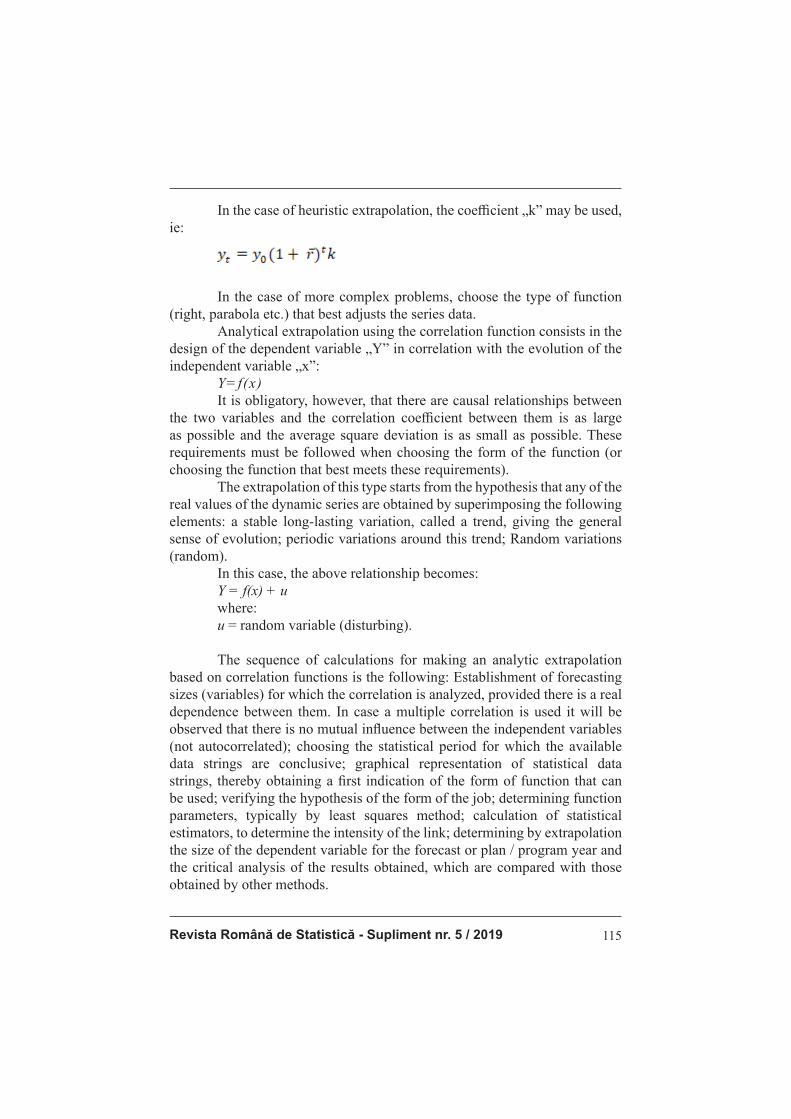
Revista Română de Statistică - Supliment nr. 5 / 2019 115
In the case of heuristic extrapolation, the coeffi cient „k” may be used,
ie:
In the case of more complex problems, choose the type of function
(right, parabola etc.) that best adjusts the series data.
Analytical extrapolation using the correlation function consists in the
design of the dependent variable „Y” in correlation with the evolution of the
independent variable „x”:
Y=f(x)
It is obligatory, however, that there are causal relationships between
the two variables and the correlation coeffi cient between them is as large
as possible and the average square deviation is as small as possible. These
requirements must be followed when choosing the form of the function (or
choosing the function that best meets these requirements).
The extrapolation of this type starts from the hypothesis that any of the
real values of the dynamic series are obtained by superimposing the following
elements: a stable long-lasting variation, called a trend, giving the general
sense of evolution; periodic variations around this trend; Random variations
(random).
In this case, the above relationship becomes:
Y = f(x) + u
where:
u = random variable (disturbing).
The sequence of calculations for making an analytic extrapolation
based on correlation functions is the following: Establishment of forecasting
sizes (variables) for which the correlation is analyzed, provided there is a real
dependence between them. In case a multiple correlation is used it will be
observed that there is no mutual infl uence between the independent variables
(not autocorrelated); choosing the statistical period for which the available
data strings are conclusive; graphical representation of statistical data
strings, thereby obtaining a fi rst indication of the form of function that can
be used; verifying the hypothesis of the form of the job; determining function
parameters, typically by least squares method; calculation of statistical
estimators, to determine the intensity of the link; determining by extrapolation
the size of the dependent variable for the forecast or plan / program year and
the critical analysis of the results obtained, which are compared with those
obtained by other methods.

Romanian Statistical Review - Supplement nr. 5 / 2019116
The phenomenological extrapolation consists in the analysis of the
global characteristics of the phenomenon based on the logical interpretation
of the lasting practical experience. Thus, certain „laws” of variation of the
phenomenon pursued can be broken down under the given circumstances. The
method is based on graphic representation, visualizing trends of evolution.
The result can be a straight expression expressed as a simple linear function
(Xt = a + by), and for more complex evolutions curves can be described by
exponential, logarithmic, logistic functions, etc.
The extrapolation by wrapping curves describes the dynamics of the
result of complex processes, consisting of several elements that intervene
successively in the overall evolution of the process. In other words, it consists
of adjusting (winding) a series of sequential curves.
• Interpolation method The interpolation method consists in establishing intermediate
values between two variables, ie between the baseline and the predicted end
of the forecast or plan period.
Interpolation can be done using two procedures:
- interpolation using the annual average rate established by the two
known sizes (X0 and XT) and the number of years between them:
R=(X, - Xo)/T
X�=X �+(R -T )
where:
R = annual average ratio;
XT = exogenous variable level for the fi nal year T;
X0 = the level of the base year variable;
T = number of years between the base year and the fi nal year;
Xt = the level of the variable, interpolated, for a year t, between the
base year and the fi nal year;
t = number of years between base year and year „t”.
- interpolation using average rhythms, establishing the average annual
rate between the base year and the end of the forecast and applying it from
near to near absolute values. The relationships are used:
Where from:
and:
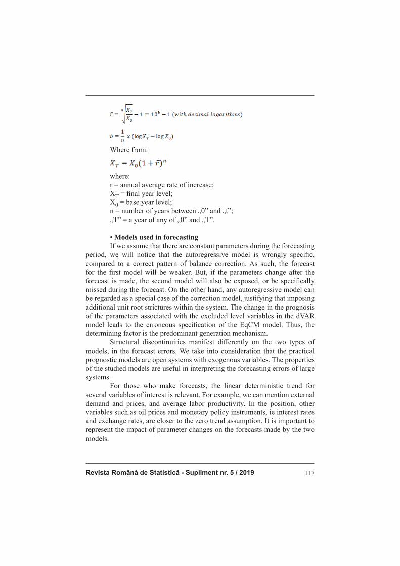
Revista Română de Statistică - Supliment nr. 5 / 2019 117
Where from:
where:
r = annual average rate of increase;
XT = fi nal year level;
X0 = base year level;
n = number of years between „0” and „t”;
„T” = a year of any of „0” and „T”.
• Models used in forecasting If we assume that there are constant parameters during the forecasting
period, we will notice that the autoregressive model is wrongly specifi c,
compared to a correct pattern of balance correction. As such, the forecast
for the fi rst model will be weaker. But, if the parameters change after the
forecast is made, the second model will also be exposed, or be specifi cally
missed during the forecast. On the other hand, any autoregressive model can
be regarded as a special case of the correction model, justifying that imposing
additional unit root strictures within the system. The change in the prognosis
of the parameters associated with the excluded level variables in the dVAR
model leads to the erroneous specifi cation of the EqCM model. Thus, the
determining factor is the predominant generation mechanism.
Structural discontinuities manifest diff erently on the two types of
models, in the forecast errors. We take into consideration that the practical
prognostic models are open systems with exogenous variables. The properties
of the studied models are useful in interpreting the forecasting errors of large
systems.
For those who make forecasts, the linear deterministic trend for
several variables of interest is relevant. For example, we can mention external
demand and prices, and average labor productivity. In the position, other
variables such as oil prices and monetary policy instruments, ie interest rates
and exchange rates, are closer to the zero trend assumption. It is important to
represent the impact of parameter changes on the forecasts made by the two
models.
Romanian Statistical Review - Supplement nr. 5 / 2019118
• Forecasting external economic relations The sphere of activity of the foreign economic relations includes: the
foreign trade itself; foreign invisible trade; services; international economic
and technical-scientifi c cooperation in the fi eld of industrial, agricultural,
construction, transport, trade, technical-scientifi c research, services, banking
operations.
Processes occur between units belonging to diff erent national
economies, even though in some cases exports do not exceed the national
boundaries of the supplier, as is the case with sales of goods and services
provided to foreign tourists on national territory.
Predictive activity includes: prospecting-forecasting activity;
transactional activity; the activity of elaborating short-term forecasts on
external economic relations.
- Economic and mathematical models used in forecasting external
economic relations
Correlation functions
- the evolution of total exports (Mt) as a function of evolution of
national income generated or GDP.
M t = f(V)
- the evolution of exports, using its share in the volume of national
income created or GDP (Kmt) as an optional trend function:
M t = Vt x Kmt
- the evolution of exports by branches and sub-branches with the same
functions, but using branch indicators;
- the evolution of exports by sub-sectors, product groups and main
products by means of normative indexes: export to one million lei production
of goods; export to one million tons of cereals; export of machines, appliances,
means of transport to 1000 pieces of products and so on;
- the evolution of total imports (Nt) as a function of evolution of GNP
(Pt), given that the import is involved both in intermediate production and in
the creation of the fi nal product:
N t = f (Pt)
- the evolution of imports using the import coeffi cient in the GNP
volume (Knt) as an optional trend function:
N t = Pt x K„t.
The matrix model (network) reveals the country’s current goods and
services with the outside; can be synthetically represented as follows:
where:
Revista Română de Statistică - Supliment nr. 5 / 2019 119
= the characteristic coeffi cient of the importing country ‚j’ during
the forecast period;
= the volume X of the goods and services currents in the country
of origin ‚i’ to the country ‚j’ in the forecast year t;
= the volume of the same currents in the base year t0;
= the characteristic coeffi cient of the exporting country ‚i’ during
the forecast period.
The gravitational model is conceived by taking into account the
degree of economic development and the economic distance between the
partners from the point of view of the exporting country. The generalized
expression of the gravitational model is as follows:
where:
Xij = volume X of goods and services currents in the exporting country
‚i’ to the importing country ‚j’;;
Vi = national income per capita of the exporting country „i”;
Vj = national income per capita of the importing country „j”;
kij = the coeffi cient expressing the economic distance between the
partners;
α = elasticity of the country’s export „i” in relation to its own national
income per capita;
β = the elasticity of the country’s import „j” in relation to its own
national income per capita.
With the help of the forecast, the composition, the dynamics and the
effi ciency of some actions to be performed are predetermined by means and
specifi c means. Prefi guration is a broad outline of what is going to happen, it
is usually done in the fi rst phases when determining the great lines of action,
the trend. Predetermination is a more complex forecast, multiple options are
taken into account, varied techniques are considered, outcome maximization
is analyzed and risks are minimized, and optimal solutions are weighed.
All forecasting predictions: forecasts, strategies, plans, programs, etc.
must combine the deterministic elements with the random ones, as the future
is both conditional and necessary.
Romanian Statistical Review - Supplement nr. 5 / 2019120
Conclusion The quantitative techniques can measure deterministic elements, ie
those caused by the cause-eff ect relationship, but can not identify random
elements. Deterministic elements are those causes that over time have had
the same eff ects, while random elements have either occurred in the past
but sporadically, or are unpredictable risks that may occur at any time in
the present or future. Several categories of forecasts are identifi ed from this
point of view: predictions under risk conditions, predictions under uncertainty
conditions, uncertainties in terms of ambiguity. In the case of risk forecasts,
the level of risk and possible types of outcomes is anticipated, but the extent
to which a result can be predicted can not be predicted. In simple situations of
this case, decisions are made with minimal risk, and in more complex cases
decisions are made with the correct ratio between the possible risk and the
cost of the risk. In the case of uncertainty forecasts, neither the results nor the
degree of achievement are known. In these cases, other information is also
used to determine the margin for producing some results. Under ambiguity
predictions, the uncertainty is caused by irrelevant data that make it diffi cult
or impossible to estimate the probability of producing a phenomenon.
References 1. Anghelache, C., Mitruţ, C., Voineagu, V. (2013). Statistică macroeconomică:
sistemul conturilor naţionale. Editura Economică, Bucureşti
2. Anghelache, C., Anghel, M.G., Jweida, I.J., Popovici, M. and Stanciu, E. (2016).
Theoretical notions of statistical estimation. Romanian Statistical Review
Supplement, 11, 120-126
3. Anghelache, C. (2008). Tratat de statistică teoretică şi economică, București:
Editura Economică
4. Benjamin, C., Herrard, N., Houée-Bigot, M., Tavéra, C. (2010). Forecasting with
an Econometric Model, Springer
5. Carroll, Ch. (2003). Macroeconomic Expectations of Households and Professional
Forecasters. Quarterly Journal of Economics, 118 (1), 269-298
6. Clark, T., Ravazzolo, F. (2015). Macroeconomic Forecasting Performance
under Alternative Specifi cations of Time-Varying Volatility. Journal of Applied
Econometrics, 30 (4), 551–575
7. Eckela, C., Philip J., Grossman, P. (2008). Forecasting risk attitudes: An
experimental study using actual and forecast gamble choices. Journal of Economic
Behavior & Organization, 68 (1), 1–17
8. Lucas, R.E. Jr. (2003). Macroeconomic Priorities. American Economic Review, 93
(1), 1-14
9. Pesaran, H., Pick, A., Pranovich, M. (2013). Optimal forecasts in the presence of
structural breaks. Journal of Econometrics, 177 (2), 134-152
10. Wilms, I., Croux, C. (2016). Forecasting using sparse cointegration. International
Journal of Forecasting. 32 (4), October–December 2016, 1256–1267.

Revista Română de Statistică - Supliment nr. 5 / 2019 121
The Analysis of the Firm Based on the Statistical Indicators
Prof. Radu Titus MARINESCU PhD ([email protected])
„Artifex”University of Bucharest
Doina AVRAM Ph.D Student ([email protected])
Bucharest University of Economic Studies
Cristian OLTEANU PhD Student ([email protected])
Bucharest University of Economic Studies
Maria MIREA PhD Student ([email protected])
Bucharest University of Economic Studies
Abstract The purpose of any economic activity at the micro, meso,
macroeconomic or even family level is the progress, well-being of the members
of the organization conducting that activity. This welfare, this progress to be
appreciated needs to be measured, evaluated, compared, a process that, at the
enterprise level, is achieved through value and / or non-value data. The results
of the economic activity at the company level are obtained by carrying out the
production and marketing activities, ie the activities of achieving the goods and
services necessary to meet the individual and social needs, and this activity
is measured by value and non-value data, which is repeated regularly takes
the form of statistical indicators of economic results. The statistical analysis
of this activity on the basis of physical and synthetic indicators is performed
with the purpose of substantiating the production and marketing program
for the following periods, establishing strategic objectives for the company’s
development. The information provided by the statistical and economic analysis
is used both by the company’s managers in the decision-making process and by
the fi nancial and credit institutions to determine the fi rm’s ability to deal with
maturity payments. The characterization of the results of the economic activity
implies the use of a system of result indicators, which include both indicators
of physical production and synthetic - money indicators.
Keywords: microeconomics, indicator, analysis, company, decision-
making process
JEL Classifi cation: C10, D23, D24
Romanian Statistical Review - Supplement nr. 5 / 2019122
Introducere Indicatorii fi zici sunt legaţi de specifi cul activităţii ramurii economice căreia îi aparţine agentul economic, ei fi ind diferiţi în industrie faţă de agricultură, construcţii, transporturi, comerţ sau turism. În interiorul ramurilor, indicatorii sunt diferiţi pe grupe şi subgrupe de activităţi. Încadrarea unei fi rme într-o ramură de activitate sau alta se efectuează după principiul preponderenţei volumului activităţii In accepţiunea specialiştilor în domeniu, pentru a analiza procesele de producţie, echilibrarea resurselor cu utilizarea bunurilor economice, subiectele economice se agregă pe ramuri, deci pe tipuri de activităţi. Ramurile sunt unităţi considerate cu producţie omogenă, care produc acelaşi produs sau o grupă de produse asemănătoare. Folosirea acestui criteriu permite analiza relațiilor de ordin tehnico economic în procesul de producţie, independent de contextul instituţional în care se desfăşoară acestea. Utilizarea acestui criteriu în Sistemul Conturilor Naţionale permite alcătuirea tabelului de intrări - ieşiri şi, pe baza lui, analiza legăturilor dintre ramuri.
Literature review Adamopoulos (2011) măsoară costul transportului în corelație cu diferențele de venit între țări. Anghel, Anghelache și Samson (2017) au analizat o serie aspecte metodologice privind comparabilitatea indicatorilor de rezultate. Anghelache (2008), precum și Anghelache și Anghel (2016) au prezentat și au analizat principalii indicatori statistici utilizați în analizele economice. Anghelache, Mitruţ și Voineagu (2013) au studiat elementele fundamentale ale statisticii macroeconomice. Anghelache și Capanu (2000) au cercetat indicatorii statistici utilizați în studiile micro şi macroeconomice. Harrison, McLaren și McMillan (2011) au abordat noțiuni privind comerțul. Newbold, Karlson și Thorne (2010) au tratat aspecte privind statistica pentru afaceri. Papa (2013) a realizat o analiză comparativă a strategiilor privind securitatea transportului maritim la nivelul Statelor Unite și al Uniunii Europene. Sheard (2014) a efectuat un studiu privind situația aeroporturilor și ocuparea forței de muncă în mediul urban.
Metodologia cercetării, date, rezultate şi discuţii • Indicatorii fi zici pentru fi rmele cu activitate industrială Producţia industrială, potrivit defi niţiei INS, este rezultatul direct şi util al agenţilor economici cu activitate industrială, precum şi a subunităţilor asimilate acestora, fi ind caracterizată prin: este rezultatul activităţii directe, nefi ind luate în considerare rezultatele indirecte, cum sunt materialele refolosibile, resturile de materii prime etc.; este rezultatul activităţii utile,
Revista Română de Statistică - Supliment nr. 5 / 2019 123
nefi ind astfel incluse rebuturile; este rezultatul activităţii proprii a agenţilor
economici, deci nu se vor include bunurile achiziţionate din afara unităţii şi
livrate ca atare, fără nici o prelucrare; este rezultatul activităţii industriale,
deci nu se vor include rezultatele din alte activităţi (agricole, de comert,
construcţii etc.) desfăşurate ca extraprofi l.
După gradul de fi nisare, elementele incluse în producţia industrială
sunt:
- Produsele fi nite, reprezentând acele produse a căror prelucrare a
fost terminată în unitatea respectivă şi sunt destinate livrării la alţi agenţi
economici sau consumate în sectorul de investiţii sau în cele neindustriale
din respectiva unitate.
- Semifabricate reprezintă produse obţinute din producţia proprie,
care au parcurs unul sau mai multe stadii de prelucrare şi care, fi e trec la
următoarele secţii pentru tenninarea prelucrării în vederea obţinerii unui
produs fi nit, fi e sunt livrate ca atare la alţi agenţi economici.
- Producţia neterminată reprezintă un element intermediar între
materia primă şi semifabricat, ori între semifabricat şi produs fi nit, reprezentând
producţia al cărei proces de execuţie, fi nisaj sau montaj, nu a fost terminat,
procesul tehnologic fi ind în curs de derulare. Valoarea producţiei neterminate
se include în volumul rezultatelor activităţii economice al unei perioade ca
sold, deci ca diferenţă între volumul stocului de producţie netenninată la
sfârşitul perioadei N2 şi cel de la începutul perioadei N1, evaluarea fi ind
efectuată la nivelul costurilor de producţie.
- Lucrările (serviciile) industriale includ activităţi prestate pentru alţi
agenţi economici, dar şi pentru sectoare neindustriale din propria unitate,
ori pentru investiţii, lucrări care au drept scop: restabilirea valorii de utilizare
a unor produse ori ridicarea performanţelor calitative ale unor produse
existente, prin operaţii de fi nisare,vopsire etc.
Producţia fi zică industrială măsoară rezultatele obţinute în procesul
de producţie sub expresie fi zico - materială „naturală”, exprimând cantităţile
diferitelor bunuri materiale şi nemateriale (produse fi nite, semifabricate,
servicii şi lucrări industriale), realizate de un agent economic într-o anumită
perioadă de timp. Producţia fi zică industrială este un „indicator vectorial”,
componentele sale interpretându-se şi judecându-se distinct, după specifi c şi
destinaţie, acestea neputând fi totalizate sau agregate.
Exprimarea fi zică a rezultatelor activităţii este legată de principalele
particularităţi şi caracteristici specifi ce ale diferitelor valori de întrebuinţare,
fi ind efectuată: în unităţi naturale (fi zice): de lungime, suprafaţă, greutate,
capacitate, concentraţie, număr de exemplare etc; în unităţi natural -
convenţionale, prin transformarea în produse echivalente (ex: cărbunele, în

Romanian Statistical Review - Supplement nr. 5 / 2019124
cărbune de o anumită putere calorică, tractoarele, în tractoare convenţionale
de o anumită putere etc.); în unităţi de muncă.
Consider că producţia fi zică înglobează rezultatele activităţii
economice, realizate la nivelul fi rmei, structurate după unitatea de măsură
fi zico - materială în care se exprimă. Pentru cuantifi carea producţiei în
unităţi naturale trebuie să poată fi identifi cată o mulţime omogenă de produse
din punctul de vedere al caracteristicilor lor tehnico - economice şi al utilităţii
lor. Cuantifi carea în unităţi naturale reprezintă baza aplicării tuturor celorlalte
forme de cuantifi care a producţiei.
Avantajul metodei îl constituie exactitatea cu care refl ectă volumul
activităţii economice pentru un anumit tip de produs. Dezavantajul metodei
stă în sfera sa limitată de cuprindere.
Dacă un produs i este realizat de mai multe secţii sau verigi
organizatorice aparţinând aceluiaşi producător, sau de mai mulţi producători,
varietatea acestora fi ind notată cu j ( j = ) , atunci volumul fi zic total al
producţiei pentru produsul i, agregarea pe verticală, este:
Agregarea volumului fi zic este posibilă numai pentru mulţimea
producătorilor de produse de acelaşi tip, nu şi pentru varietatea produselor. Se
constată că nu pot fi însumate produsele decât pe verticală, deoarece numai
aşa sunt prezente caracteristici de omogenitate şi anume, caracteristici fi zico
tehnologice asemănătoare. Chiar dacă unitatea de măsură a produselor este
aceeaşi, totuşi, nu este permisă însumarea lor.
O altă formă de cuantifi care a producţiei industriale o reprezintă
unităţile natural convenționale
Cuantifi carea în unități natural - convenționale se aplică unei mulţimi
de produse omogene sub aspectul utilităţii, dar eterogene din punctul de
vedere al caracteristicilor tehnico - economice. Omogenitatea se realizează
cu un coefi cient , care poate fi ales în funcţie de caracteristica principală
a produsului, de timpul unitar de realizare şi de preţ.
Coefi cientul de transformare se determină ca raport între
caracteristica produsului i de transformat şi caracteristica produsului etalon:
unde: CPT = caracteristica produsului de transformat;
CPE = caracteristica produsului etalon.

Revista Română de Statistică - Supliment nr. 5 / 2019 125
Dacă se consideră varietatea produselor în raport cu nivelul
caracteristicilor tehnice ( i = ) , atunci pentru întreaga producţie omogenă
din punctul de vedere al utilităţii produselor, modelul devine:
Dacă luăm în considerare şi posibilitatea ca produsul, într-o gamă variată, să fi e realizat în cadrul unor secţii de producţie sau verigi organizatorice aparţinănd unui singur producător sau considerând că mai mulţi producători realizează produsele respective, iar varietatea acestora se notează cu j ( j = ) , atunci pentru întregul volum al producţiei relaţia de determinare devine:
este coefi cientul de echivalenţă determinat ca raport între caracteristica produsului i şi caracteristica produsului etalon şi serveşte astfel drept coefi cient de omogenizare a producţiei. Această metodă lărgeşte sfera de cuprindere a producţiei, dar prezintă dezavantajul că se limitează la o mulţime de produse ce au aceeaşi utilitate. Se utilizează ca formă de cuantifi care a producţiei industriale şi unităţilor de timp de muncă. În acest caz, elementul de omogenizare al producţiei îl reprezintă timpul aferent realizării unui produs, exprimat în ore. Datorită acestui fapt, metoda este considerată , de unii autori, ca fi ind cea mai fi delă formă de refl ectare a producţiei, dar sfera
sa de aplicabilitate este redusă datorită volumului mare de muncă necesar.
Dacă se consideră varietatea produselor i= , cea a operaţiunilor
tehnologice la care sunt supuse produsele k = , varietatea secţiilor de
producţie ale aceluiaşi producător j = , atunci modelul de determinare a
volumului producţiei în unităţi de timp de muncă devine:
relaţie în care:
= timpul unitar aferent operațiunii tehnologice , pentru obținerea
produsului i la nivelul verigii organizatorice j.
Avantajele şi funcţiile indicatorilor fi zici în procesul managerial:
- forma simplă de exprimare permite identifi carea şi urmărirea
comenzilor şi contractelor;

Romanian Statistical Review - Supplement nr. 5 / 2019126
- pot fi efectuate corelaţii cu alţi indicatori ai activităţii economice cum sunt consumul de materii prime, materiale, energie, timp de muncă, fond de salarii;
- se poate calcula randamentul folosirii factorilor de producţie (productivitatea naturală, consumul unitar de capital fi x şi circulant etc.);
- pot fi efectuate corelări cu indicatorii fi nanciari ai activităţii economice cum sunt costurile, profi tul etc.
- cu ajutorul lor se poate cacula indicele volumului fi zic al producţiei pe grupe de produse;
- sunt folosiţi la elaborarea de indicatori utili în comparaţii internaţionale, referitoare la nivelul dezvoltării economice (ex: producţia de energie electrică/locuitor).
Indicatorul fi zic al producţiei industriale prezintă şi o serie de limite: - nu se referă la volumul total al activităţii desfăşurate de un agent
economic, neincluzând, - de exemplu, soldul producţiei neterminate, care în întreprinderile
cu ciclu lung de fabricaţie, poate înregistra valori mari; - nu permite evidenţierea nivelului tehnic al producţiei; - nu diferenţiază rezultatele în funcţie de performanţele calitative ale
produselor; - nu pot fi caracterizate sintetic rezultatele nici la nivelul agenţilor
economici şi nici la niveluri superioare de agregare. Principala defi cienţă a indicatorilor fi zici o reprezintă faptul că nu pot fi agregaţi, neputând fi totalizaţi pentru produse sau servicii diferite exprimate în unităţi de măsură diferite. Pentru aceasta se utilizează exprimarea bănească. În cazul metodei de cuantifi care a productiei industriale în unităti valorice, elementul de omogenizare îl constituie preţul unui produs i practicat de către un producător j (pij)
La nivelul produsului, valoarea producției fi zice este: qij pij. La nivelul unui producător, valoarea producției fi zice este:
La nivelul grupului de producători, valoarea producției fi zice este:
Revista Română de Statistică - Supliment nr. 5 / 2019 127
Exprimarea producţiei în unităţi alorice permite includerea tuturor componentelor producţiei, a tuturor produselor şi a tuturor producătorilor în indicatorii producţiei. Ca atare, principalul avantaj al metodei îl constituie sfera sa largă de cuprindere, iar dezavantajul său este reprezentat de nivelul preţului, care poate avantaja sau dezavantaja anumiţi producători. Ca exemplu, se consideră acelaşi volum fi zic al producţiei, pentru care, producătorul ce practică un preţ mai ridicat este mai avantajat sub aspectul valorii producţiei realizate. Exprimarea fi zică a indicatorilor de rezultate economice permite calcularea lor pe fi ecare ramură de activitate. Astfel, în rândurile următoare am prezentat indicatorii fi zici din agricultură, construcţii şi transporturi. - Indicatorii fi zici pentru fi rmele agricole se calculează pe activităţi distincte. - Indicatorii fi zici în activitatea de construcţii se stabilesc pentru fi ecare categorie de lucrări au categorie de obiecte de construcţii: clădiri industriale, construcţii agro-tehnice, construcţii social-culturale, clădiri de locuit etc. - Indicatori fi zici pentru caracterizarea activităţii întreprinderilor din transporturi. Întreprinderile din domeniul transportului au ca obiect de activitate deplasarea persoanelor şi a bunurior cu ajutorul unor vehicule. în raport cu mijloacele de transport utilizate şi cu obiectul transportului, există următorii indicatori ai fi rmelor de transport: a. Indicatorii transportului feroviar de mărfuri se calculează pe baza
documentului intitulat „scrisoare de trăsură” care furnizează informaţii necesare la calculul prestaţiilor şi al veniturilor, la nivelul costurilor transporturilor.
b. Indicatorii transportului auto de mărfuri. Documentele contabile care furnizează informaţiile utilizate la calculul indicatorilor sunt foaia de parcurs şi scrisoarea de transport, prin care se confi rmă transportul şi se efectuează decontările între benefi ciar şi întreprinderea de transport.
c. Indicatorii transportului naval de mărfuri. În cadrul relaţiilor externe legate de transportul mărfurilor, transportul naval este preponderent. Informaţiile pentru calculul indicatorilor specifi ci acestui tip de transport sunt prezentate în documentele specifi ce numite contract de navlosire şi conosament, care certifi că mărfurile încărcate pe navă. Activităţile desfăşurate în domeniul portuar, prin diversitatea lor implică determinarea unui ansamblu de indicatori specifi ci activității portuare, cum sunt: numărul de nave operate, indicator care depinde de capacitatea de trafi c a
Romanian Statistical Review - Supplement nr. 5 / 2019128
radei (parte a portului în care navele sunt în aşteptare); cantitatea
de marfă ce tranzitează prin port şi care este dependentă de capacitatea frontului de dane (frontul de acostare şi operare a navelor), de capacitatea depozitelor a instalaţiilor şi utilajelor ca şi de capacitatea căilor ferate şi a drumurilor din incinta portului.; trafi cul portuar exprimă, în tone, cantitatea mărfurilor intrate şi ieşite în şi din porturi fl uviale şi maritime.
d. Indicatorii trafi cului aerian de mărfuri. Transportul de mărfuri pe calea aerului prezintă o pondere redusă în totalul activităţii de transport, datorită valorii ridicate şi caracterului perisabil al mărfurilor ce fac obiectul transportului, dar şi distanţelor mari ce trebuiesc parcurse într-un timp foarte scurt. Documentul care furnizează datele privind marfa, expeditorul şi destinatarul pentru calculul indicatorilor este fractul aerian.
e. Indicatori ai transportului de călători în trafi cul feroviar.
Indicatorii activități de transport sunt calculați pe baza documentelor de evidență numite legitimații de călătorie.
f. Indicatorii transportului naval de călători: numărul călătorilor transportați (mii călători); parcursul călătorilor (km).
g. Indicatorii transportului prin conducte petroliere magistrale se referă la greutatea produselor petroliere pompate prin conducte petroliere magistrale şi ajunse la destinatie. În activitatea de transport se utilizează şi o serie de indicatori natural convenționali, precum tona - km convențională în transportul feroviar, auto şi naval, iar în trafi cul aerian se utilizează indicatorul călătorul - km
convențional. În unități convenționale se calculează volumul de transport ( ) prin relația:
reprezintă parcursul mărfurilor în tone-km fi zice;
reprezintă parcursul călătorilor (în călători-km); - coefi cientul de transformare, care se stabileşte pe baza raportului între costul trafi cului care se transformă şi costul trafi cului bază de comparaţie. Valorile coefi cientului de transformare sunt: - în trafi cul feroviar 1 tonă-km=1 călător-km; - în auto 1 tonă-km = 0,18 călători-km; - în trafi cul fl uvial 1tonă-km = 5,8 călători-km; - în trafi cul maritim 1 tonă-km = 4,966 călători-km; - în trafi cul aerian 1 tonă - km =12,5 călători-km.
Revista Română de Statistică - Supliment nr. 5 / 2019 129
• Indicatori fi zici pentru măsurarea rezultatelor activităţii agenţilor economici din sfera comerţului interior şi alimentaţiei publice
Agenţii economici cu activitate de comerţ asigură închiderea circuitului economic, mijlocesc raporturile dintre furnizori şi benefi ciari: sub forma schimbului de mărfuri. Pentru continuitatea activităţii de aprovizionare şi desfacere la nivelul unităţilor de comerţ cu ridicata şi cu amănuntul se formează stocuri. Principalii indicatori ai stocurilor de mărfuri sunt: - nivelul absolut al stocului;
- nivelul mediu al stocului ( ), care se calculează ca medie cronologică ponderată a valorilor stocului (St) la diferite momente de timp și intervalele în
zile dintre momente (ti);
- rata stocului se stabilește ca raport între mărimea stocului existent
într-un moment al perioadei analizate (S) și desfacerile înregistrate în acea
perioadă (Q):
Indicatorul exprimă mărimea stocului necesar la fi ecare 1000 lei (RON) încasări din vânzarea mărfurilor. Rata stocului se poate calcula și pe
baza stocului mediu al perioadei cercetate (lună, trimestru sau an):
- siguranța vânzărilor se poate exprima cu ajutorul indicatorului stoc
- exprimat în zile - rulaj (s) pentru unitățile comerțului cu ridicata sau stoc -
exprimar în zile - desfacere (S ) pentru unitățile comerțului cu amănuntul:
sau
în care:
S- stocul existent la un moment dat;
R- rulajul total al lunii, trimestrului sau anului;
Q- desfacerea sau vânzarea cu amănuntul;
11Z- numărul de zile ale perioadei respective.
Acesta este indicatorul care estimează numărul de zile în care
desfacerea este asigurată fără a face vreo reaprovizionare a unităţii analizate.
Romanian Statistical Review - Supplement nr. 5 / 2019130
- viteza de circulație a mărfurilor (V) este indicatorul care arată în
câte zile se epuizează stocul mediu, dacă se menține desfacerea medie zilnică.
- stocul mediu al perioadei cercetate;
- desfacerea medie zilnică
- rotația stocurilor (nr) este un indicator calitativ al activităţii
întreprinderilor comerciale, el arătând de câte ori se reînnoiesc stocurile în
perioada cercetată sau de câte ori volumul desfacerilor este acoperit de stocul
mediu, și se calculează prin una din relaţiile următoare:
sau
• Indicatori pentru măsurarea rezultatelor activității fi rmelor de comerț exterior
Prezentarea activităţii agenţilor economici cu activitate de comerţ
exterior se realizează prin următorii indicatori fi zici:
- volumul mărfurilor exportate/importate;
- cota parte a exportului în productie (g) se stabileşte prin relaţia:
în care:
E - volumul producției exportate;
Q - întreaga producție.
- rata dependenței de piețele externe de aprovizionare (m) exprimă
cât din consumul de materii prime (M) se asigură din import (I) sau cât din
resursele interne (R) sunt completate din import.
• Indicatori ai activităţii pentru fi rmele de turism
Rezultatele activităţii fi rmelor de turism îl reprezintă produsul turistic,
care este o prestaţie în domeniul serviciilor. Principalii indicatori ai acestei
activităţi sunt:
- numărul total de turiști ;
- numărul total de zile - turist ( ,
z - durata activității turistice exprimată în zile

Revista Română de Statistică - Supliment nr. 5 / 2019 131
- numărul mediu de turiști ( )
- durata medie a sejurului
În întreprinderile care îşi desfăşoară activitatea în sectorul serviciilor, consider că pot fi calculaţi următorii indicatori de apreciere a rezultatelor activităţii economice: 1. Rata comenzilor refuzate (RCR) care exprimă promptitudinea în livrarea comenzilor şi preocuparea pentru asigurarea calităţii serviciilor prestate:
sau
2. Rata comenzilor livrate (RCL) exprimă respectul fi rmei față de solicitările clienților, dar și existența unor probleme de organizare în funcționarea fi rmei.
sau
În administrația publică,rezultatele activității desfășurate pot fi apreciate cu ajutorul următorilor indicatori: 1. Rata investițiilor fi nalizate (RIF), care exprimă efi cienţa utilizării fondurilor disponibile pentru investiţii.
2. Interesul pentru activitatea investitională (IAI) exprimă preocuparea administraţiei publice pentru obţinerea de fonduri extrabugetare destinate activităţii investiţionale.
3. Ritmicitatea utilizării fondurilor din proiecte (extrabugetare) şi concretizarea lor în investiţii fi nalizate se calculează cu rata investitiilor din proiecte fi nalizate (RIPF).
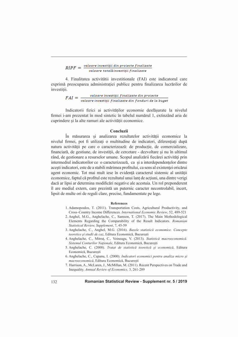
Romanian Statistical Review - Supplement nr. 5 / 2019132
4. Finalitatea activitătii investitionale (FAI) este indicatorul care
exprimă preocuparea administraţiei publice pentru fi nalizarea lucrărilor de
investiţii.
Indicatorii fi zici ai activităților economie desfășurate la nivelul fi rmei i-am prezentat în mod sintetic în tabelul numărul 1, extinzând aria de cuprindere și la alte ramuri ale activității economice.
Concluzii În măsurarea şi analizarea rezultatelor activităţii economice la nivelul fi rmei, pot fi utilizaţi o multitudine de indicatori, diferenţiaţi după natura activităţii pe care o caracterizează: de producţie, de comercializare, fi nanciară, de gestiune, de investiţii, de cercetare - dezvoltare şi nu în ultimul rând, de gestionare a resurselor umane. Scopul analizării fi ecărei activităţi prin intermediul indicatorilor ce o caracterizează, ca şi a interdependenţelor dintre aceşti indicatori, este de a stabili mărimea profi tului, ca sens al existenţei oricărui agent economic. Tot mai mult iese în evidenţă caracterul sistemic al unităţii economice, faptul că profi tul este rezultatul unui lanţ de acţiuni, una dintre verigi dacă ar lipsi ar determina modifi cări negative ale acestuia. Un rol preponderent îl are mediul extern, care prezintă un puternic caracter necontrolabil, incert, lipsit de multe ori de reguli clare, precise, fundamentate pe lege.
References 1. Adamopoulos, T. (2011). Transportation Costs, Agricultural Productivity, and
Cross–Country Income Diff erences. International Economic Review, 52, 489-521 2. Anghel, M.G., Anghelache, C., Samson, T. (2017). The Main Methodological
Elements Regarding the Comparability of the Result Indicators. Romanian
Statistical Review, Supplement, 7, 45-59 3. Anghelache, C., Anghel, M.G. (2016). Bazele statisticii economice. Concepte
teoretice şi studii de caz, Editura Economică, Bucureşti 4. Anghelache, C., Mitruţ, C., Voineagu, V. (2013). Statistică macroeconomică.
Sistemul Conturilor Naţionale, Editura Economică, Bucureşti 5. Anghelache, C. (2008). Tratat de statistică teoretică şi economică, Editura
Economică, Bucureşti 6. Anghelache, C., Capanu, I. (2000). Indicatori economici pentru analiza micro şi
macroeconomică, Editura Economică, București 7. Harrison, A., McLaren, J., McMillan, M. (2011). Recent Perspectives on Trade and
Inequality. Annual Review of Economics, 3, 261-289
Revista Română de Statistică - Supliment nr. 5 / 2019 133
8. Newbold, P., Karlson, L.W., Thorne, B. (2010). Statistics for Business and
Economics, 7th ed., Pearson Global Edition, Columbia, U.S 9. Papa, P. (2013). US and EU strategies for maritime transport security: A comparative
perspective. Transport Policy, 28, 75-85 10. Sheard, N. (2014). Airports and urban sectoral employment. Journal of Urban
Economics, 80, 133-152