simulare termocupla
11
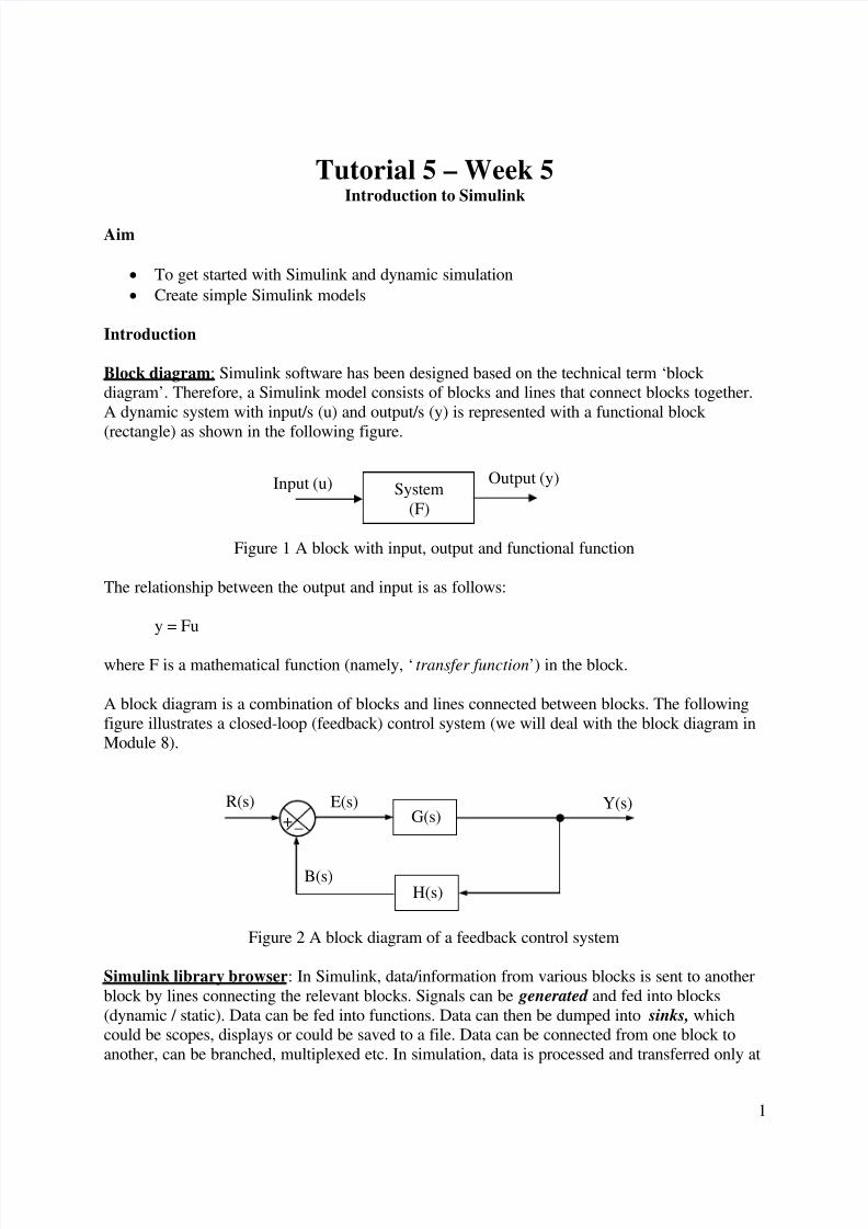
1 Tutorial 5 – Week 5 Introduction to Simulink Aim • To get started with Simulink and dynamic simulation • Create simple Simulink models Introduction Block diagram: Simulink software has been designed based on the technical term ‘block diagram’. Therefore, a Simulink model consists of blocks and lines that connect blocks together. A dynamic system with input/s (u) and output/s (y) is represented with a functional block (rectangle) as shown in the following figure. Figure 1 A block with input, output and functional function The relationship between the output and input is as follows: y = Fu where F is a mathematical function (namely, ‘ transfer function’) in the block. A block diagram is a combination of blocks and lines connected between blocks. The following figure illustrates a closed-loop (feedback) control system (we will deal with the block diagram in Module 8). Figure 2 A block diagram of a feedback control system Simulink library browser: In Simulink, data/information from various blocks is sent to another block by lines connecting the relevant blocks. Signals can be generated and fed into blocks (dynamic / static). Data can be fed into functions. Data can then be dumped into sinks, which could be scopes, displays or could be saved to a file. Data can be connected from one block to another, can be branched, multiplexed etc. In simulation, data is processed and transferred only at System (F) Output (y) Input (u) G(s) E(s) Y(s) H(s) +_ R(s) B(s)
-
Upload
roscovanul -
Category
Documents
-
view
241 -
download
0
Transcript of simulare termocupla
8/6/2019 simulare termocupla
http://slidepdf.com/reader/full/simulare-termocupla 1/10
1
Tutorial 5 – Week 5Introduction to Simulink
Aim
• To get started with Simulink and dynamic simulation• Create simple Simulink models
Introduction
Block diagram : Simulink software has been designed based on the technical term ‘block diagram’. Therefore, a Simulink model consists of blocks and lines that connect blocks together.A dynamic system with input/s (u) and output/s (y) is represented with a functional block
(rectangle) as shown in the following figure.
Figure 1 A block with input, output and functional function
The relationship between the output and input is as follows:
y = Fu
where F is a mathematical function (namely, ‘ transfer function ’) in the block.
A block diagram is a combination of blocks and lines connected between blocks. The followingfigure illustrates a closed-loop (feedback) control system (we will deal with the block diagram inModule 8).
Figure 2 A block diagram of a feedback control system
Simulink library browser : In Simulink, data/information from various blocks is sent to anotherblock by lines connecting the relevant blocks. Signals can be generated and fed into blocks(dynamic / static). Data can be fed into functions. Data can then be dumped into sinks, whichcould be scopes, displays or could be saved to a file. Data can be connected from one block toanother, can be branched, multiplexed etc. In simulation, data is processed and transferred only at
System(F)
Output (y)Input (u)
G(s)E(s) Y(s)
H(s)
+ _R(s)
B(s)
8/6/2019 simulare termocupla
http://slidepdf.com/reader/full/simulare-termocupla 2/10
2
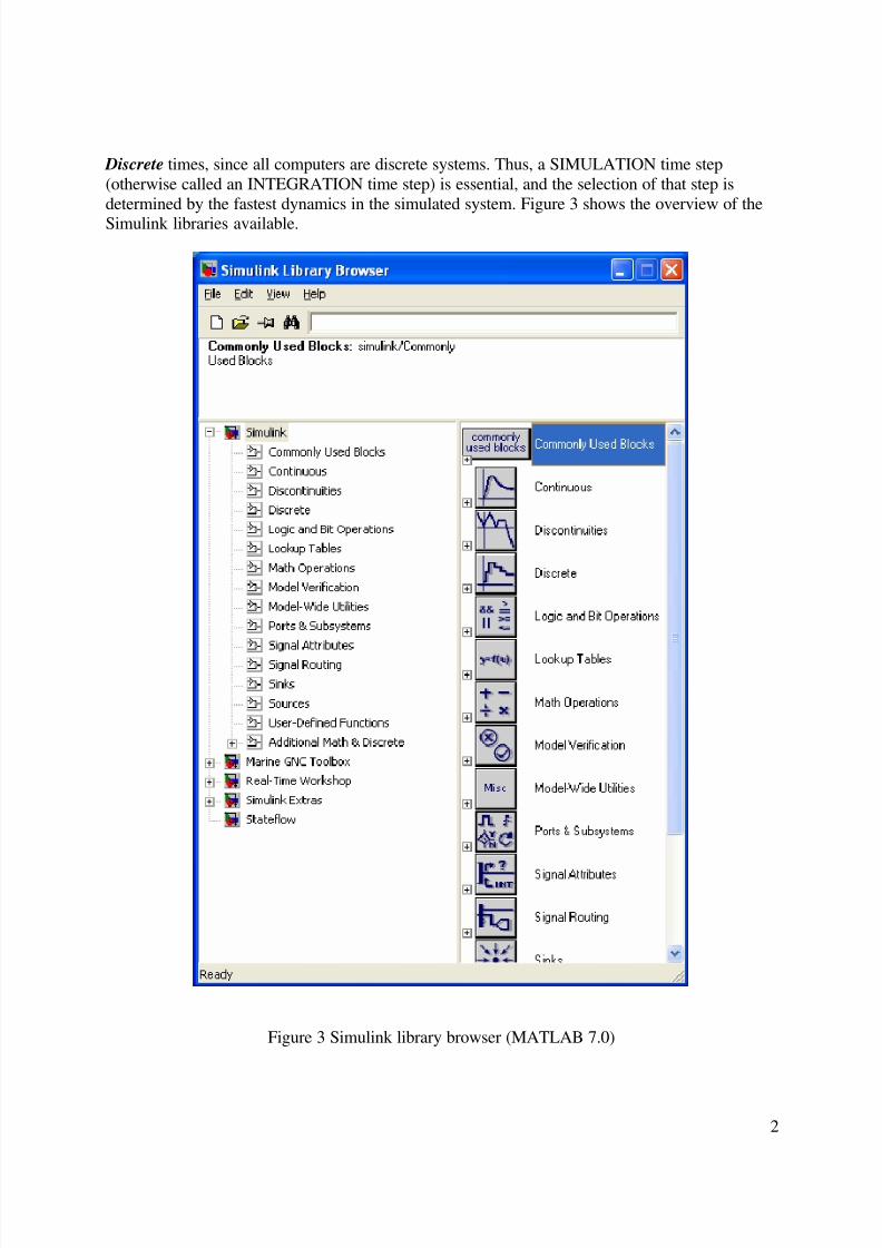
Discrete times, since all computers are discrete systems. Thus, a SIMULATION time step(otherwise called an INTEGRATION time step) is essential, and the selection of that step isdetermined by the fastest dynamics in the simulated system. Figure 3 shows the overview of theSimulink libraries available.
Figure 3 Simulink library browser (MATLAB 7.0)
8/6/2019 simulare termocupla
http://slidepdf.com/reader/full/simulare-termocupla 3/10
3
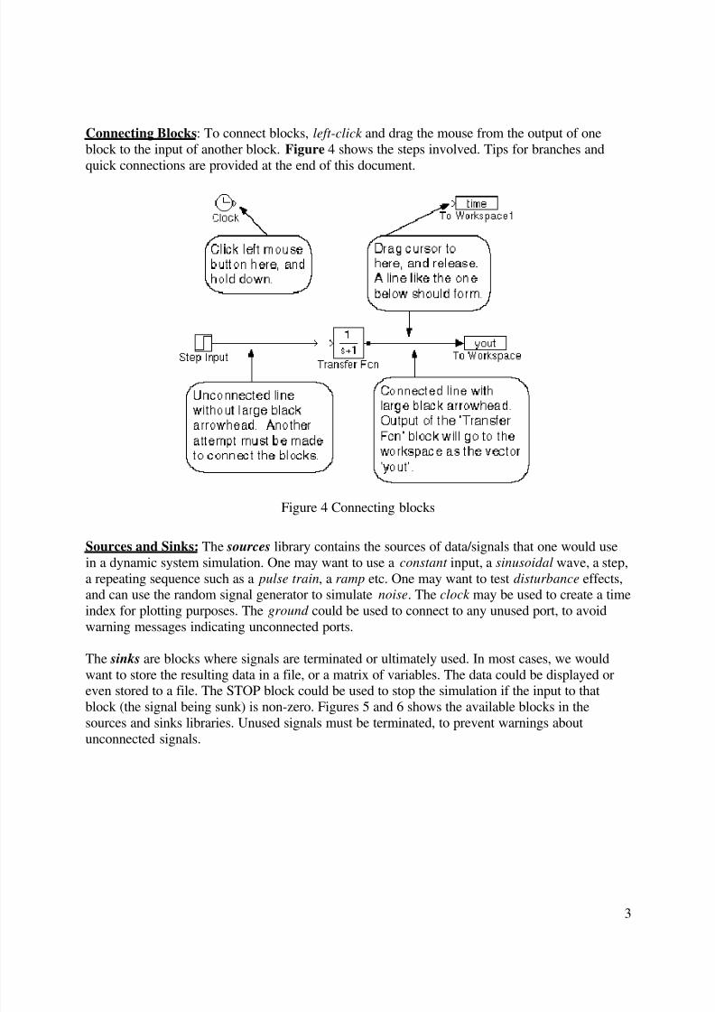
Connecting Blocks : To connect blocks, left-click and drag the mouse from the output of oneblock to the input of another block. Figure 4 shows the steps involved. Tips for branches andquick connections are provided at the end of this document.
Figure 4 Connecting blocks
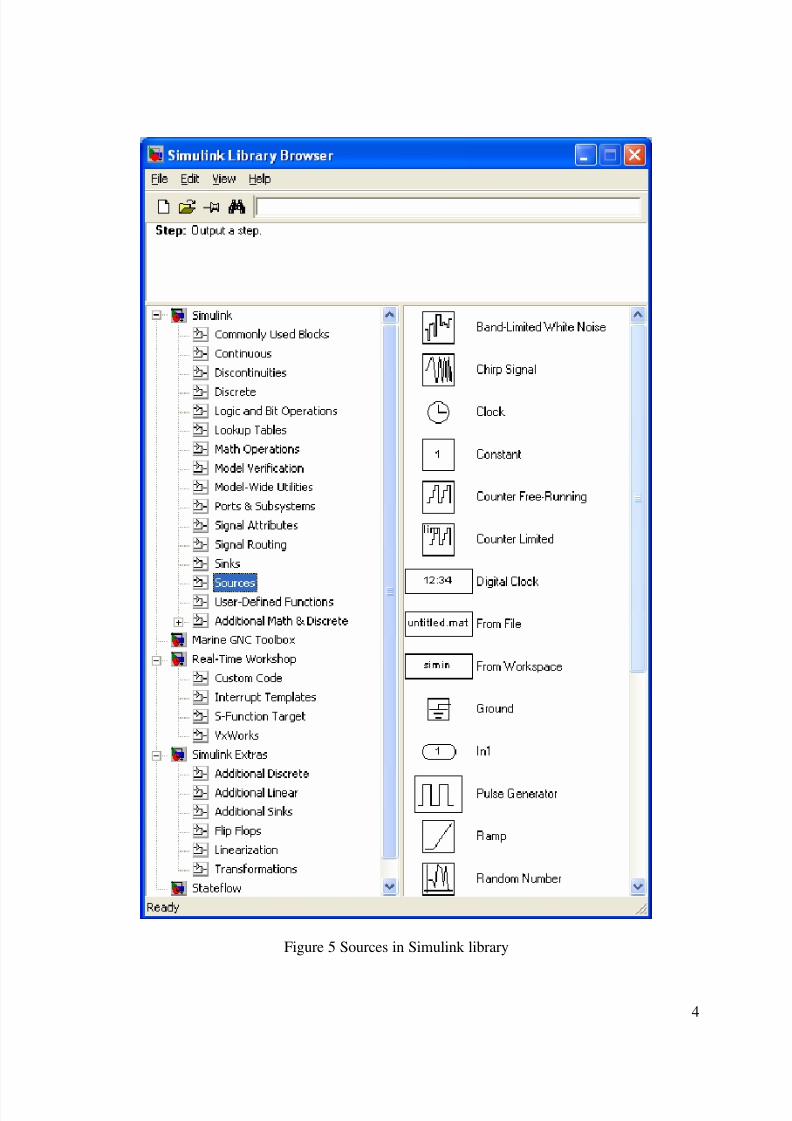
Sources and Sinks: The sources library contains the sources of data/signals that one would usein a dynamic system simulation. One may want to use a constant input, a sinusoidal wave, a step,a repeating sequence such as a pulse train , a ramp etc. One may want to test disturbance effects,and can use the random signal generator to simulate noise . The clock may be used to create a timeindex for plotting purposes. The ground could be used to connect to any unused port, to avoidwarning messages indicating unconnected ports.
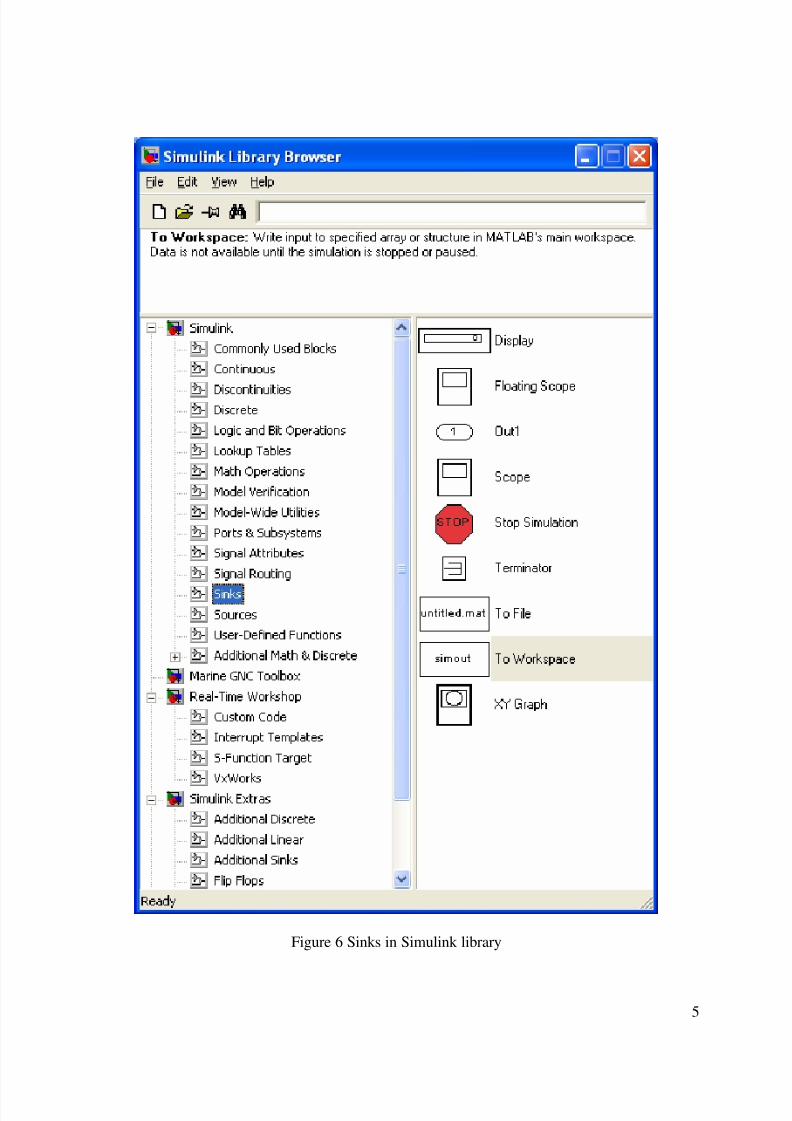
The sinks are blocks where signals are terminated or ultimately used. In most cases, we wouldwant to store the resulting data in a file, or a matrix of variables. The data could be displayed oreven stored to a file. The STOP block could be used to stop the simulation if the input to that
block (the signal being sunk) is non-zero. Figures 5 and 6 shows the available blocks in thesources and sinks libraries. Unused signals must be terminated, to prevent warnings aboutunconnected signals.
8/6/2019 simulare termocupla
http://slidepdf.com/reader/full/simulare-termocupla 4/10
4
Figure 5 Sources in Simulink library
8/6/2019 simulare termocupla
http://slidepdf.com/reader/full/simulare-termocupla 5/10
5
Figure 6 Sinks in Simulink library
8/6/2019 simulare termocupla
http://slidepdf.com/reader/full/simulare-termocupla 6/10
6
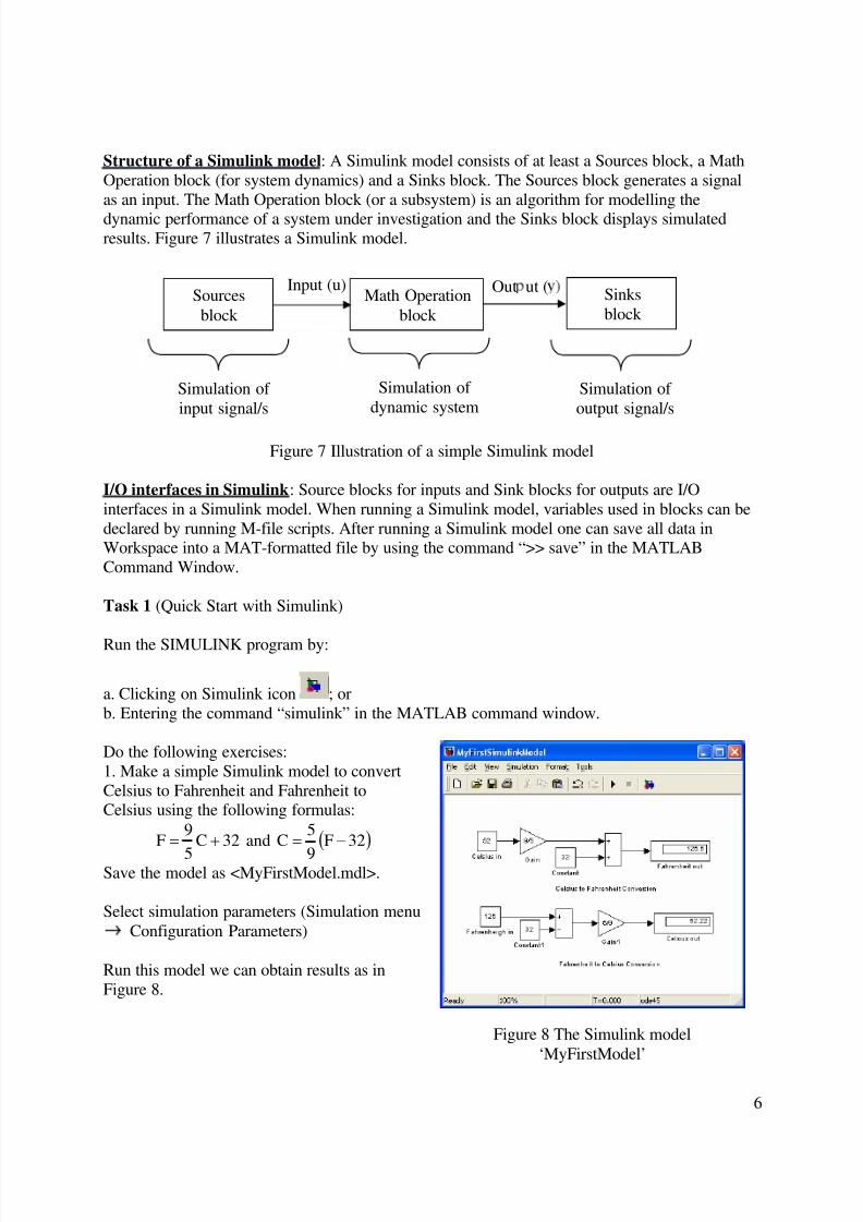
Structure of a Simulink model : A Simulink model consists of at least a Sources block, a MathOperation block (for system dynamics) and a Sinks block. The Sources block generates a signalas an input. The Math Operation block (or a subsystem) is an algorithm for modelling thedynamic performance of a system under investigation and the Sinks block displays simulatedresults. Figure 7 illustrates a Simulink model.
Figure 7 Illustration of a simple Simulink model
I/O interfaces in Simulink : Source blocks for inputs and Sink blocks for outputs are I/Ointerfaces in a Simulink model. When running a Simulink model, variables used in blocks can bedeclared by running M-file scripts. After running a Simulink model one can save all data inWorkspace into a MAT-formatted file by using the command “>> save” in the MATLABCommand Window.
Task 1 (Quick Start with Simulink)
Run the SIMULINK program by:
a. Clicking on Simulink icon ; orb. Entering the command “simulink” in the MATLAB command window.
Do the following exercises:1. Make a simple Simulink model to convertCelsius to Fahrenheit and Fahrenheit toCelsius using the following formulas:
32C5
9F += and ( )32F
9
5C −=
Save the model as <MyFirstModel.mdl>.
Select simulation parameters (Simulation menu→ Configuration Parameters)
Run this model we can obtain results as inFigure 8.
Math Operationblock
Out ut (Input (u)Sources
block Sinksblock
Simulation of input signal/s
Simulation of dynamic system
Simulation of output signal/s
Figure 8 The Simulink model‘MyFirstModel’
8/6/2019 simulare termocupla
http://slidepdf.com/reader/full/simulare-termocupla 7/10
7
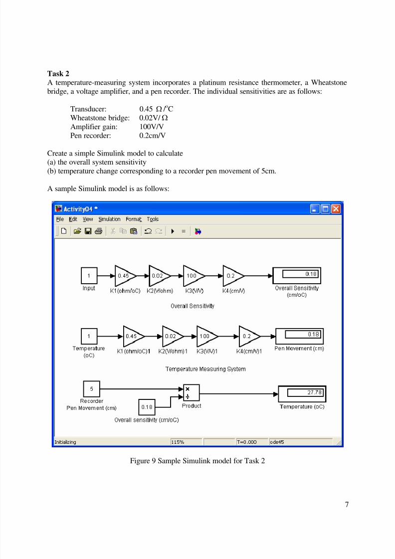
Task 2A temperature-measuring system incorporates a platinum resistance thermometer, a Wheatstonebridge, a voltage amplifier, and a pen recorder. The individual sensitivities are as follows:
Transducer: 0.45 Ω / oCWheatstone bridge: 0.02V/ Ω Amplifier gain: 100V/VPen recorder: 0.2cm/V
Create a simple Simulink model to calculate(a) the overall system sensitivity(b) temperature change corresponding to a recorder pen movement of 5cm.
A sample Simulink model is as follows:
Figure 9 Sample Simulink model for Task 2
8/6/2019 simulare termocupla
http://slidepdf.com/reader/full/simulare-termocupla 8/10
8
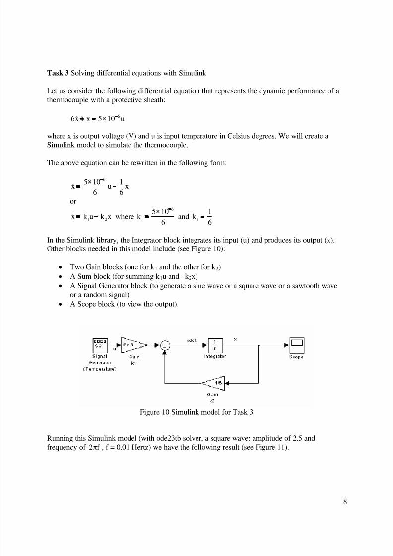
Task 3 Solving differential equations with Simulink
Let us consider the following differential equation that represents the dynamic performance of athermocouple with a protective sheath:
66x x 5 10 u+ = ×
where x is output voltage (V) and u is input temperature in Celsius degrees. We will create aSimulink model to simulate the thermocouple.
The above equation can be rewritten in the following form:
65 10 1x u x
6 6
−×
= −
or
1 2x k u k x− where6
1
5 10k
6
−×
= and 2
1k
6=
In the Simulink library, the Integrator block integrates its input (u) and produces its output (x).Other blocks needed in this model include (see Figure 10):
• Two Gain blocks (one for k 1 and the other for k 2)• A Sum block (for summing k 1u and –k 2x)• A Signal Generator block (to generate a sine wave or a square wave or a sawtooth wave
or a random signal)• A Scope block (to view the output).
Figure 10 Simulink model for Task 3
Running this Simulink model (with ode23tb solver, a square wave: amplitude of 2.5 andfrequency of 2 f π , f = 0.01 Hertz) we have the following result (see Figure 11).
8/6/2019 simulare termocupla
http://slidepdf.com/reader/full/simulare-termocupla 9/10
9
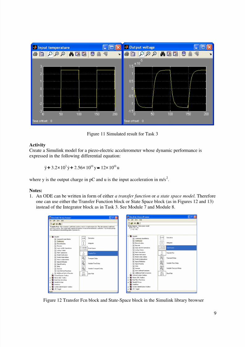
Figure 11 Simulated result for Task 3
ActivityCreate a Simulink model for a piezo-electric accelerometer whose dynamic performance isexpressed in the following differential equation:
3 10 10y 3.2 10 y 2.56 10 y 12 10 u× + × = ×
where y is the output charge in pC and u is the input acceleration in m/s 2.
Notes:1. An ODE can be written in form of either a transfer function or a state space model . Therefore
one can use either the Transfer Function block or State Space block (as in Figures 12 and 13)instead of the Integrator block as in Task 3. See Module 7 and Module 8.
Figure 12 Transfer Fcn block and State-Space block in the Simulink library browser
8/6/2019 simulare termocupla
http://slidepdf.com/reader/full/simulare-termocupla 10/10
10
Figure 12 Transfer Fcn block and State-Space block
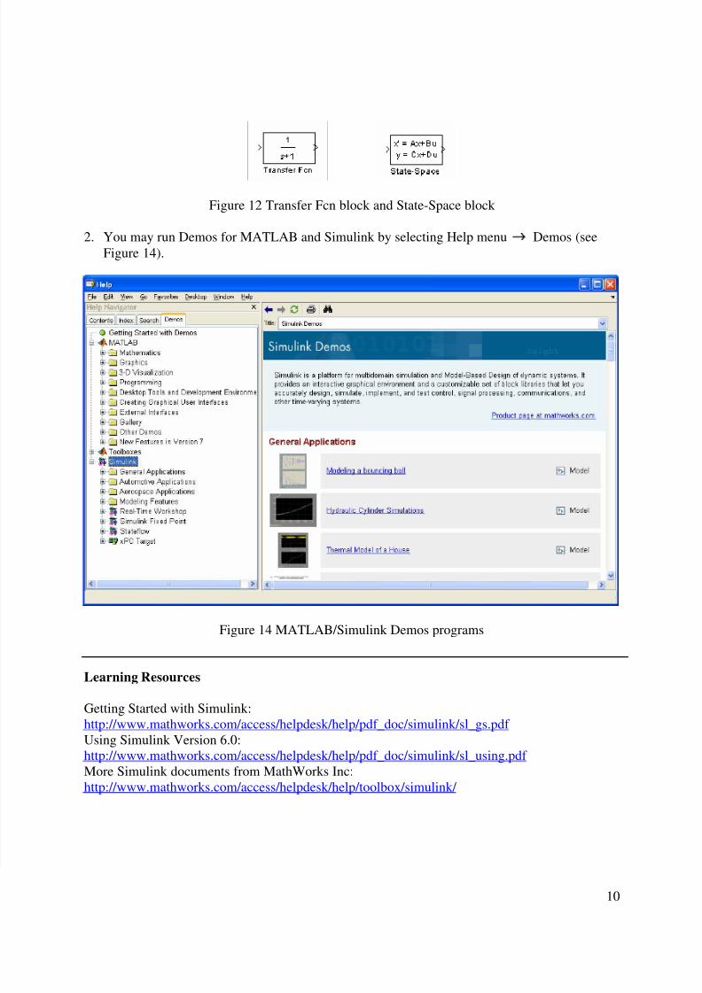
2. You may run Demos for MATLAB and Simulink by selecting Help menu → Demos (seeFigure 14).
Figure 14 MATLAB/Simulink Demos programs
Learning Resources
Getting Started with Simulink:http://www.mathworks.com/access/helpdesk/help/pdf_doc/simulink/sl_gs.pdf Using Simulink Version 6.0:http://www.mathworks.com/access/helpdesk/help/pdf_doc/simulink/sl_using.pdf More Simulink documents from MathWorks Inc:http://www.mathworks.com/access/helpdesk/help/toolbox/simulink/