Redactor şef / Editor in chief Prof.dr.ing. Ioan Naforniţă Colegiul de redacţie / Editorial Board:

Prof. dr. ing. Virgil Tiponuţ Prof. dr. ing. Alexandru Isar

Conf. dr. ing. Dan Lacrămă Conf. dr. ing. Dorina Isar Prof. dr. ing. Traian Jurcă

Conf. dr. ing. Aldo De Sabata As. ing. Kovaci Maria - secretar de redacţie Colectivul de recenzare / Advisory Board:

Prof. dr. ing. Ioan Naforniţă, UP Timişoara Prof. dr. ing. Monica Borda, UT Cluj-Napoca Prof. dr. ing. Brânduşa Pantelimon, UP Bucureşti Prof. dr. ing. Ciochină Silviu, UP Bucureşti Prof. dr. ing. Dumitru Stanomir, UP Bucureşti Prof. dr. ing. Vladimir Creţu, UP Timişoara Prof. dr. ing. Virgil Tiponuţ, UP Timişoara

Buletinul Ştiinţific

al Universităţii "Politehnica" din Timişoara

Seria ELECTRONICĂ ŞI TELECOMUNICAŢII

TRANSACTIONS ON ELECTRONICS AND COMMUNICATIONS

Tom 48(62), Fascicola 1, 2003

SUMAR

ELECTRONICĂ APLICATĂ

Adrian Popovici, Viorel Popescu: "Development of DSP Real Time Control Software for Power Converters"… … … … … … … … … … … … … ...… … … … … … … … … .. 3 Adrian Popovici, Viorel Popescu: "A Low Signal Model for Development of Matrix Converters Control Strategies"… … … … … … … … … … … … … ... ... ... ... ... … … ... … … … . 9

INSTRUMENTAŢIE

Rudolf Kortvelyessy, Alimpie Ignea, Adrian Mihaiuţ : "Studiul produselor de intermodulaţie de ordinul III din liniile de transmisiune"…………………… ... ... ... ... ... ... ... ... … … … … … … … … … 13

Daniel Belega, Dan Stoiciu : " Accurate Harmonics Analyzer"…………………… ... ... ... ... ... ... ... .. .17 Adrian Vârtosu : "Frequency Multiplier with Varactor Diode"…………………… ... ... ... .23 Daniel Belega : "ADC Testing by Beat Frequency and Envelope Methods"…… ... … … 27

Septimiu Mischie : "Generation of a user definable waveform using a HM 8130 Function Generator connected to an IBM-PC Computer via IEEE 488 Interface"... … .33

1

TELECOMUNICAŢII

Georgeta Budura: "Some Aspects Regarding Frequency Analysis of the Nonlinear Systems".……………………….. ... ... ... ... ... ... ... ... ... ... ... ... ... ... ... ... … … 37 Georgeta Budura, Corina Botoca: "Analysis and Modeling of Systems with Nonlinearities"… … … … … 43 Corina Botoca, Georgeta Budura: "Neural Networks Intelligent Tools for Telecommunications Problems"… … … … … … … … … … … … … … … … … … … … … … … … … … … … .51 Corina Botoca: "Some Aspects of Cellular Neural Networks and Their Applications"… … … … … … … … … … … … … … … … … … … … … … … … … … … … .59 Marius Oltean, Miranda Naforniţă: "Word Error Rate Statistics of a DFT- based MCM System in FSF Channels"… … … … … … … … … … … … … … … … … … … … … … … ..67 Corina Naforniţă, Alexandru Isar: "Digital Watermarking of Still Images using the Disctrete Wavelet Transform"… … … … … … … … … … … … … … … … … … … … … … … 73 Marius Sălăgean, Mirela Bianu, Cornelia Gordan: "Instantaneous Frequency and its Determination"… … … … … … … ..79 Dan Gh. T. Popa: "Doppler Signal Extractor"… … … … … … … … … … … … … … … 85 Mircea Coşer: "TRIZ – a short presentation"… … … … … … … … … … … … … … ..89

2

Buletinul Ştiinţific al Universităţii "Politehnica" din Timişoara

Seria ELECTRONICĂ şi TELECOMUNICAŢII TRANSACTIONS on ELECTRONICS and COMMUNICATIONS

Tom 48 (62), Fascicola 1, 2003

Development of DSP Real Time Control Software for Power Converters

Adrian Popovici Viorel Popescu 1

1 Facultatea de Electronică şi Telecomunicaţii, Departamentul Electronică Aplicată Bd. V. Pârvan Timişoara 1900

Abstract - This paper describes the possibility of using an simulation model for power converters in development of DSP real time control software for power converters. A simulation model for matrix converters using Simulink software package is presented. This model is based on the switching function concept. The switching functions are synthesized in accordance with SLM (scalar line to line voltages modulation) algorithm. These function can use for generate real time signals for control of matrix converter.

I. INTRODUCTION The recent developments in electrical drive technology are motivated by increasing requirements of industrial applications for higher performance, better reliability and lower cost. They are due to advances in several areas in particular power electronics, control theory and microprocessor technology. Today power electronic systems have attained an unusual high degree of complexity so that their control becomes more and more sophisticated. The control of a power electronic system requires several function of a different nature: signal filtering, regulation, drive signal generation, measurement, monitoring, protection. For a long time the implementation of these function has relied mainly on analog technology using a hardwired approach. The development of microprocessors has promoted the use of digital technology in the control of power electronic system using a software approach that provides greater flexibility and better performance. The development of microprocessor based control systems become more and more complex so that sophisticated tools are required for the design, simulation and testing of the target systems. For many years analog controllers have dominated the control of power electronic systems. But the new requirements from industrial applications are such that they cannot adequately respond from lack of processing capabilities. It has been proven that that the modular design approach provides in general a high flexibility concerning analysis design construction test and debugging of the system.

The development of real time control software can be done following three main stages: simulation, off line development and real time integration. In the first stage

the control algorithms are developed using a simulation environment such as Matlab. The algorithms and control configurations are tested and debugged using a high level language that facilitates the development task. In the second stage the control tasks are written as several modules which are tested individually first. Then the modules are combined and tested in an offline context. Finally in the third stage the control modules are integrated with a real time operating system and the whole is tested and debugged in real time conditions. The control software can be written by using assembler language or high level language. Assembler has always been recognized as an effective programming language for real time control systems because it gives access to the processor internal structure. A major drawback of assembler programming resides in the processor dependence of developed software. At present C language is widely accepted as a programming language for real time control systems because of its portability and effectiveness in manipulating hardware resources. [1]

The advantage of digital control for power converters is that the software program can be changed and revised by changing a few line of text in a data file. User friendly, but powerfull development tools allow fast program debugging enabling programmers to focus their efforts on the software design rather than on the nuances of the development system. Circuit simulation programs can help evaluate the results of possible abnormalities. The simulation program is a powerful tool for developing circuits and even system level design [2].

II. SIMULATION OF POWER ELECTRONICS

CIRCUITS New designs of power electronics systems are

the norm due to new applications and the lack of standardization in specifications is because of varying customer demands. Accurate simulation is necessary to minimize costly repetitions of designs and breadboarding and hence reduce the overall cost and the concept to production time lag. Simulation may give a

3

comprehensive and impressive documentation of system performance that gives a competitive edge to a company using the simulation. It is normally more cheaper to do a trough analysis than to build a the actual circuit. A simulation can discover possible problems and determine optimal parameters, increasing the possibility of getting the prototype right the first time. Simulation can be used to optimize the performance objective by letting the simulation search over a large number of variables. New circuit concepts and parameter variations are easily tested. Changes in the circuit topology are implemented with no cost. It is possible to simplify parts of circuits in order to focus on a specific portion of the circuit. Switches are the most widely used elements in power electronic simulations because all semiconductor devices are modeled as switches. Switch models are the origin of the most of the difficulty for numerical routines used in simulation program. They may cause convergence errors and can initiate numerical oscillations. At the core of each simulation are differential and algebraic equations that describe the system. The implementation of ideal model switch is simply a short circuit in its on state and an open circuit in the off state.

Matlab is an equations solver program and contain sophisticated toolboxes for control analysis and design. The controller can be designed based on the performance specifications and than it is translated into C and finally into assembly language for programming the digital signal processors.

Simulink is a software package that works in Matlab environment. The user needs only to select the required blocks from a large library of functions and assign the parameter values in the blocks. Simulink also allows the use of variable names in these blocks which are passed through a block mask. Matlab is a technical computing environment whose basic data element is self-dimensioning matrix. It combines fast numerical capabilities with excellent graphics using a command syntax that is quite intuitive. Matlab is useful for developing and modifying algorithms, particularly those which are heavy in matrix operation.

The simulation model proposed in this paper is analytically based on the switching function concept. A lot of research works in switching power converters has demonstrated that the transfer or switching function concept is a powerful tool in understanding and optimizing the performance of converters [3], [4], [5]. Accurate models for the converter switch are not required at this level of simulation. The transfer function is the instantaneous relation between the input and the output variables. A general converter has a current and a voltage transfer function, both defined by the same switching function applied to the control port. The signals applied to the control input port are switching functions. By using the concept of switching functions, and with the assumptions of no losses no parasitic reactive elements in the converter, the functional representation of various types of converters

is derived. The mathematical expression can contain the variable time and any mixture of voltage and currents.

This model employs Simulink software package [6]. Simulink is an extension to Matlab and allows graphical block diagram modeling of dynamic systems. It is easier to develop a power converter system simulation using this software package, as many components of the system are included in the Simulink block diagram library. This makes simulation design more efficient and allows other interested parties to understand the operation of the power converter more easily than a programming language implementation. It is easy to capture and displays results using the predefined blocks for these purposes. One of the essential feature of this simulation model is that it can be run on a DSP platform, with an appropriate C compiler for real time application [7]. This feature greatly reduces development time of a prototype model.

Another advantage of using Simulink is the possibility of using the Power System Blockset software. It is a convenient tool to simulate electrical circuits containing power electronic devices, since it detects very accurately the instants at which discontinuities and switchings occur. It was designed to simulate power systems and electric devices. Because of their stiffness and nonlinearity, modern power systems require simulation tools based on performance integration methods [8].

Another facility of using Simulink in power electronics is that with the same software, a particular circuit can be designed and analyzed at different system and subsystem levels, i.e. at levels of power switch, the converter circuit and the converter system.

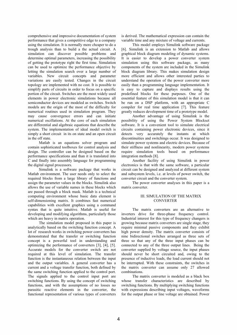
The power converter analyses in this paper is a matrix converter.

III. SIMULATION OF THE MATRIX

CONVERTER The matrix converters are an alternative to

inverters drive for three-phase frequency control. Industrial interest for this type of frequency changers is growing because matrix converters are single stage, they require minimal passive components and they exhibit high power density. The matrix converter consists of nine bidirectional switches arranged as three sets of three so that any of the three input phases can be connected to any of the three output lines. Being the converter supplied by voltage source, the input phases should never be short circuited and, owing to the presence of inductive loads, the load current should not be interrupted. With these constraints, the switches in the matrix converter can assume only 27 allowed combinations.

The matrix converter is modeled as a black box whose transfer characteristics are described by switching functions. By multiplying switching functions with expressions describing input voltages, waveforms for the output phase or line voltage are obtained. Power

4

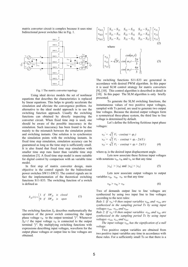
matrix converter circuit is complex because it uses nine bidirectional power switches like in Fig. 1.

Using ideal device models the set of nonlinear equations that describes the characteristics is replaced by linear equations. This helps to greatly accelerate the simulation and alleviate the convergence problem. An alternative to the ideal model approach is to use the switching function approach. Usually the switching functions can obtained by directly inspecting the converter circuit. When fixed time step is used, one should be aware of the possible inaccuracy in the simulation. Such inaccuracy has been found to be due mainly to the mismatch between the simulation points and switching instants. One solution is to synchronize the simulation points with the switching instants. In fixed time step simulation, simulation accuracy can be guaranteed as long as the time step is sufficiently small. It is also found that fixed time step simulation with smaller time step runs faster than variable time step simulation [3]. A fixed time step model is more suitable for digital control by comparison with an variable time model. In first step of matrix converter design, main objective is the control signals for the bidirectional power switches SW11-SW33. The control signals are in fact the implementation of the theoretical switching functions S11-S33. The switching function of a switch is defined as

⎩⎨⎧

=openisSWif

closedisSWif)t(S

jk

jkjk 0

1 (1)

The switching function Sjk describes mathematically the operation of the power switch connecting the input phase voltage vIk to the output terminal "j". Whenever Sjk=1 the input voltage vIk is connected to the output terminal "j". By multiplying switching functions with expressions describing input voltages, waveform for the output phase voltages or output line to line voltages are obtained.

⎥⎥⎥

⎦

⎤

⎢⎢⎢

⎣

⎡⋅

⎥⎥⎥

⎦

⎤

⎢⎢⎢

⎣

⎡

−−−−−−−−−

=⎥⎥⎥

⎦

⎤

⎢⎢⎢

⎣

⎡

3

2

1

133312321131

332332223121

231322122111

031

023

012

I

I

I

vvv

SSSSSSSSSSSSSSSSSS

vvv

(2) where

( )

⎥⎥⎥⎥⎥⎥⎥

⎦

⎤

⎢⎢⎢⎢⎢⎢⎢

⎣

⎡

⎟⎠⎞

⎜⎝⎛ −

⎟⎠⎞

⎜⎝⎛ −=

⎥⎥⎥

⎦

⎤

⎢⎢⎢

⎣

⎡

343

22

3

2

1

πω

πω

ω

tcos

tcos

tcos

Vvvv

I

I

I

I

I

I

I

(3)

The switching functions S11-S33 are generated in accordance with desired PWM algorithm. In this paper it is used SLM control strategy for matrix converters [9], [10]. This control algorithm is described in detail in [10]. In this paper The SLM algorithm is only briefly presented.

To generate the SLM switching functions, the instantaneous values of two positive input voltages, sampled with Ts period, are used to generate two output line voltages. Because the desired output voltages form a symmetrical three-phase system, the third line to line voltage is determined by default.

Let’s define the following fictitious input phase voltages:

vI1' = 2 VI ⋅ cos(ωIt + ϕI )

vI2' = 2 VI ⋅ cos(ωIt + ϕI - 2π/3 )

vI3' = 2 VI ⋅ cos(ωIt + ϕI + 2π/3 ) (4)

where ϕI is the desired input displacement angle.

Lets now associate these fictious input voltages with notations vIa, vIb and vIc so that any time

|vIa| > |vIb| and |vIa| > |vIc| (5) Lets now associate output voltages to output

variables v0p, v0q, v0r so that any time

v0p > v0q > v0r (6) Two of demands output line to line voltages are synthesized by using two input line to line voltages according to the next rules: Rule 1: If vIa >0 then output variables v0pq and -v0rp are synthesized in the sampling period Ts by using input voltages vIab, -vIca and vIaa. Rule 2: If vIa <0 then output variables -v0rp and v0qr are synthesized in the sampling period Ts by using input voltages -vIab, vIca and vIaa.

The input voltage vIaa has the signification of a null voltage.

Two positive output variables are obtained from two positive input variables any time in accordance with these rules. For a sufficiently small Ts so that there is a

Fig. 1 The matrix converter topology

vI1

iI3

iI2

iI1

vI2

vI3vI31

vI23

vI12

v023

v012

v031

i01vF01

i02

i03

vF03

vF02

Z2

Z1

Z3

SW11

SW12

SW13

SW21

SW22

SW23

SW31

SW32

SW33

5

very little variation of the input and output waveforms inside each switching sequence, the demands output line to line voltages can be synthesized in each sampling period by using two input line to line voltage as follows: v0pq = hpqb ⋅ vIab + hpqc ⋅ (-vIca)+ hpqa ⋅ vIaa (7)

-v0rp = hrpb ⋅ vIab + hrpc ⋅ (-vIca)+ hrpa ⋅ vIaa (8)

for vIa > 0 or

-v0rp = hrpb ⋅ (-vIab) + hrpc ⋅ vIca + hrpa ⋅ vIaa (9)

v0qr = hqrb ⋅ (-vIab) + hqrc ⋅ vIca + hqra ⋅ vIaa (10) for vIa < 0. These coefficients ”h” can be calculated as

follows:

|vv|)cos(V

vh IbcIab

IIL

pqpqb −⋅

⋅=

ϕ20

3

|vv|)cos(V

vh IcaIbc

IIL

pqpqc −⋅

⋅=

ϕ20

3

hpqa = 1 - hpqb - hpqc

|vv|)cos(V

vh IbcIab

IIL

prrpb −⋅

⋅=

ϕ20

3

|vv|)cos(V

vh IcaIbc

IIL

prrpc −⋅

⋅=

ϕ20

3

hrpa = 1 - hrpb - hrpc (11) for vIa >0.

Similar expressions can be obtained for vIa <0. The coefficients “h” named transfer functions, represent in fact the duty cycle of the “S” switching functions in a sample period Ts.

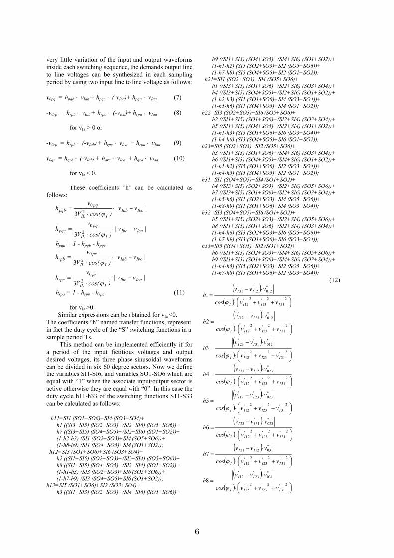
This method can be implemented efficiently if for a period of the input fictitious voltages and output desired voltages, its three phase sinusoidal waveforms can be divided in six 60 degree sectors. Now we define the variables SI1-SI6, and variables SO1-SO6 which are equal with “1” when the associate input/output sector is active otherwise they are equal with “0”. In this case the duty cycle h11-h33 of the switching functions S11-S33 can be calculated as follows:

h11=SI1 (SO1+SO6)+SI4⋅(SO3+SO4)+ h1 ((SI3+SI5) (SO2+SO3)+(SI2+SI6) (SO5+SO6))+ h7 ((SI3+SI5) (SO4+SO5)+(SI2+SI6) (SO1+SO2))+ (1-h2-h3) (SI1 (SO2+SO3)+SI4 (SO5+SO6))+ (1-h8-h9) (SI1 (SO4+SO5)+SI4 (SO1+SO2)); h12=SI3 (SO1+SO6)+SI6 (SO3+SO4)+ h2 ((SI1+SI5) (SO2+SO3)+(SI2+SI4) (SO5+SO6))+ h8 ((SI1+SI5) (SO4+SO5)+(SI2+SI4) (SO1+SO2))+ (1-h1-h3) (SI3 (SO2+SO3)+SI6 (SO5+SO6))+ (1-h7-h9) (SI3 (SO4+SO5)+SI6 (SO1+SO2)); h13=SI5 (SO1+SO6)+SI2 (SO3+SO4)+ h3 ((SI1+SI3) (SO2+SO3)+(SI4+SI6) (SO5+SO6))+

h9 ((SI1+SI3) (SO4+SO5)+(SI4+SI6) (SO1+SO2))+ (1-h1-h2) (SI5 (SO2+SO3)+SI2 (SO5+SO6))+ (1-h7-h8) (SI5 (SO4+SO5)+SI2 (SO1+SO2)); h21=SI1 (SO2+SO3)+SI4 (SO5+SO6)+ h1 ((SI3+SI5) (SO1+SO6)+(SI2+SI6) (SO3+SO4))+ h4 ((SI3+SI5) (SO4+SO5)+(SI2+SI6) (SO1+SO2))+ (1-h2-h3) (SI1 (SO1+SO6)+SI4 (SO3+SO4))+ (1-h5-h6) (SI1 (SO4+SO5)+SI4 (SO1+SO2)); h22=SI3 (SO2+SO3)+SI6 (SO5+SO6)+ h2 ((SI1+SI5) (SO1+SO6)+(SI2+SI4) (SO3+SO4))+ h5 ((SI1+SI5) (SO4+SO5)+(SI2+SI4) (SO1+SO2))+ (1-h1-h3) (SI3 (SO1+SO6)+SI6 (SO3+SO4))+ (1-h4-h6) (SI3 (SO4+SO5)+SI6 (SO1+SO2)); h23=SI5 (SO2+SO3)+SI2 (SO5+SO6)+ h3 ((SI1+SI3) (SO1+SO6)+(SI4+SI6) (SO3+SO4))+ h6 ((SI1+SI3) (SO4+SO5)+(SI4+SI6) (SO1+SO2))+ (1-h1-h2) (SI5 (SO1+SO6)+SI2 (SO3+SO4))+ (1-h4-h5) (SI5 (SO4+SO5)+SI2 (SO1+SO2)); h31=SI1 (SO4+SO5)+SI4 (SO1+SO2)+ h4 ((SI3+SI5) (SO2+SO3)+(SI2+SI6) (SO5+SO6))+ h7 ((SI3+SI5) (SO1+SO6)+(SI2+SI6) (SO3+SO4))+ (1-h5-h6) (SI1 (SO2+SO3)+SI4 (SO5+SO6))+ (1-h8-h9) (SI1 (SO1+SO6)+SI4 (SO3+SO4)); h32=SI3 (SO4+SO5)+SI6 (SO1+SO2)+ h5 ((SI1+SI5) (SO2+SO3)+(SI2+SI4) (SO5+SO6))+ h8 ((SI1+SI5) (SO1+SO6)+(SI2+SI4) (SO3+SO4))+ (1-h4-h6) (SI3 (SO2+SO3)+SI6 (SO5+SO6))+ (1-h7-h9) (SI3 (SO1+SO6)+SI6 (SO3+SO4)); h33=SI5 (SO4+SO5)+SI2 (SO1+SO2)+ h6 ((SI1+SI3) (SO2+SO3)+(SI4+SI6) (SO5+SO6))+ h9 ((SI1+SI3) (SO1+SO6)+(SI4+SI6) (SO3+SO4))+ (1-h4-h5) (SI5 (SO2+SO3)+SI2 (SO5+SO6))+ (1-h7-h8) (SI5 (SO1+SO6)+SI2 (SO3+SO4)); (12)

( )( ) ⎟

⎠⎞⎜

⎝⎛ ++⋅

⋅−=

231

223

212

01212311

'I

'I

'II

*'I

'I

vvvcos

vvvh

ϕ

( )( ) ⎟

⎠⎞⎜

⎝⎛ ++⋅

⋅−=

231

223

212

01223122

'I

'I

'II

*'I

'I

vvvcos

vvvh

ϕ

( )( ) ⎟

⎠⎞⎜

⎝⎛ ++⋅

⋅−=

231

223

212

01231233

'I

'I

'II

*'I

'I

vvvcos

vvvh

ϕ

( )( ) ⎟

⎠⎞⎜

⎝⎛ ++⋅

⋅−=

231

223

212

02312314

'I

'I

'II

*'I

'I

vvvcos

vvvh

ϕ

( )( ) ⎟

⎠⎞⎜

⎝⎛ ++⋅

⋅−=

231

223

212

02323125

'I

'I

'II

*'I

'I

vvvcos

vvvh

ϕ

( )( ) ⎟

⎠⎞⎜

⎝⎛ ++⋅

⋅−=

231

223

212

02331236

'I

'I

'II

*'I

'I

vvvcos

vvvh

ϕ

( )( ) ⎟

⎠⎞⎜

⎝⎛ ++⋅

⋅−=

231

223

212

03112317

'I

'I

'II

*'I

'I

vvvcos

vvvh

ϕ

( )( ) ⎟

⎠⎞⎜

⎝⎛ ++⋅

⋅−=

231

223

212

03123128

'I

'I

'II

*'I

'I

vvvcos

vvvh

ϕ

6

( )( ) ⎟

⎠⎞⎜

⎝⎛ ++⋅

⋅−=

231

223

212

03131239

'I

'I

'II

*'I

'I

vvvcos

vvvh

ϕ (13)

Being the converter supplied by voltage source, the input phases should never be short circuited and, owing to the presence of inductive loads, the load current should not be interrupted. Thus one and only one of the switches for each output terminal must be closed at any instant of time. This means that if two duty cycles are calculated the third is determined implicitly. In this case it is sufficiently to use six timers for generating the necessary PWM signals for the bidirectional switches control. Then all the nine switching functions can be generate by a decoder.

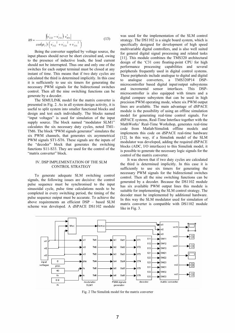
The SIMULINK model for the matrix converter is presented in Fig. 2. As in all system design activity, it is useful to split system into smaller functional blocks and design and test each individually. The blocks named “input voltages” is used for simulation of the input supply source. The block named “modulator SLM1” calculates the six necessary duty cycles, noted TM1-TM6. The block “PWM signals generator” simulates the six PWM channels, that generates six asymmetrical PWM signals ST1-ST6. These signals are the inputs of the “decoder” block that generates the switching functions S11-S33. They are used for the control of the “matrix converter” block.

IV. DSP IMPLEMENTATION OF THE SLM

CONTROL STRATEGY

To generate adequate SLM switching control signals, the following issues are decisive: the control pulse sequence must be synchronised to the input sinusoidal cycle, pulse time calculations needs to be completed in every switching period, the timing of the pulse sequence output must be accurate. To achieve the above requirements an efficient DSP – based SLM scheme was developed. A dSPACE DS1102 module

was used for the implementation of the SLM control strategy. The DS1102 is a single board system, which is specifically designed for development of high speed multivariable digital controllers, and is also well suited for general digital signal processing and related tasks [11]. This module combines the TMS320 architectural design of the ‘C31 core floating-point CPU for high performance processing capabilities and several peripherals frequently used in digital control systems. These peripherals include analogue to digital and digital to analogue converters, a TMS320P14 DSP-microcontroller based digital input/output subsystems and incremental sensor interfaces. This DSP-microcontroller is also equipped with timers and a digital compare subsystem that can be used in high precision PWM operating mode, where six PWM output lines are available. The main advantage of dSPACE module is the possibility of using an offline simulation model for generating real-time control signals. For dSPACE systems, Real-Time Interface together with the MathWorks’ Real-Time Workshop, generates real-time code from Matlab/Simulink offline models and implements this code on dSPACE real-time hardware [12]. In this way, if a Simulink model of the SLM modulator was developed, adding the required dSPACE blocks (ADC, I/O interfaces) to this Simulink model, it is possible to generate the necessary logic signals for the control of the matrix converter.

It was shown that if two duty cycles are calculated the third is determined implicitly. In this case it is sufficiently to use six timers for generating the necessary PWM signals for the bidirectional switches control. Then all the nine switching functions can be generated by a decoder. Because the DS1102 module has six available PWM output lines this module is suitable for implementing the SLM control strategy. The decoder must be implemented by additional hardware. In this way the SLM modulator used for simulation of matrix converter is compatible with DS1102 module like in Fig. 3.

Fig. 2 The Simulink model for the matrix converter

7

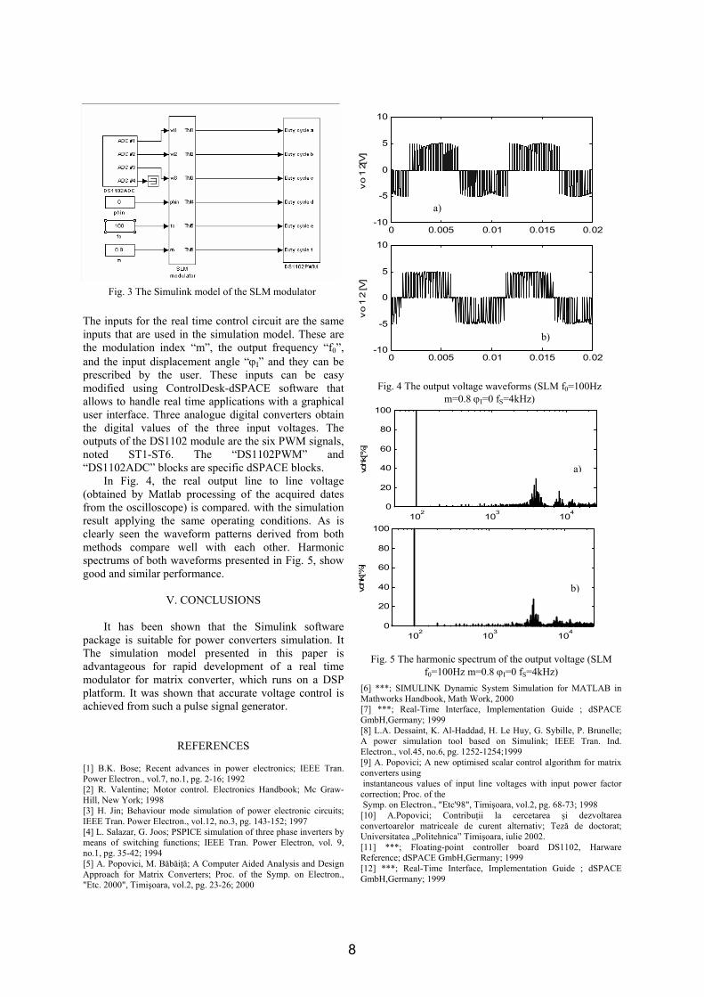
The inputs for the real time control circuit are the same inputs that are used in the simulation model. These are the modulation index “m”, the output frequency “f0”, and the input displacement angle “ϕI” and they can be prescribed by the user. These inputs can be easy modified using ControlDesk-dSPACE software that allows to handle real time applications with a graphical user interface. Three analogue digital converters obtain the digital values of the three input voltages. The outputs of the DS1102 module are the six PWM signals, noted ST1-ST6. The “DS1102PWM” and “DS1102ADC” blocks are specific dSPACE blocks. In Fig. 4, the real output line to line voltage (obtained by Matlab processing of the acquired dates from the oscilloscope) is compared. with the simulation result applying the same operating conditions. As is clearly seen the waveform patterns derived from both methods compare well with each other. Harmonic spectrums of both waveforms presented in Fig. 5, show good and similar performance.

V. CONCLUSIONS

It has been shown that the Simulink software package is suitable for power converters simulation. It The simulation model presented in this paper is advantageous for rapid development of a real time modulator for matrix converter, which runs on a DSP platform. It was shown that accurate voltage control is achieved from such a pulse signal generator.

REFERENCES [1] B.K. Bose; Recent advances in power electronics; IEEE Tran. Power Electron., vol.7, no.1, pg. 2-16; 1992 [2] R. Valentine; Motor control. Electronics Handbook; Mc Graw-Hill, New York; 1998 [3] H. Jin; Behaviour mode simulation of power electronic circuits; IEEE Tran. Power Electron., vol.12, no.3, pg. 143-152; 1997 [4] L. Salazar, G. Joos; PSPICE simulation of three phase inverters by means of switching functions; IEEE Tran. Power Electron, vol. 9, no.1, pg. 35-42; 1994 [5] A. Popovici, M. Băbăiţă; A Computer Aided Analysis and Design Approach for Matrix Converters; Proc. of the Symp. on Electron., "Etc. 2000", Timişoara, vol.2, pg. 23-26; 2000

[6] ***; SIMULINK Dynamic System Simulation for MATLAB in Mathworks Handbook, Math Work, 2000 [7] ***; Real-Time Interface, Implementation Guide ; dSPACE GmbH,Germany; 1999 [8] L.A. Dessaint, K. Al-Haddad, H. Le Huy, G. Sybille, P. Brunelle; A power simulation tool based on Simulink; IEEE Tran. Ind. Electron., vol.45, no.6, pg. 1252-1254;1999 [9] A. Popovici; A new optimised scalar control algorithm for matrix converters using instantaneous values of input line voltages with input power factor correction; Proc. of the Symp. on Electron., "Etc'98", Timişoara, vol.2, pg. 68-73; 1998 [10] A.Popovici; Contribuţii la cercetarea şi dezvoltarea convertoarelor matriceale de curent alternativ; Teză de doctorat; Universitatea „Politehnica” Timişoara, iulie 2002. [11] ***; Floating-point controller board DS1102, Harware Reference; dSPACE GmbH,Germany; 1999 [12] ***; Real-Time Interface, Implementation Guide ; dSPACE GmbH,Germany; 1999

Fig. 3 The Simulink model of the SLM modulator

102

103

104

0

20

40

60

80

100

vohk

[%]

a)

102 103 1040

20

40

60

80

100

vohk

[%]

b)

Fig. 5 The harmonic spectrum of the output voltage (SLM f0=100Hz m=0.8 ϕI=0 fS=4kHz)

0 0.005 0.01 0.015 0.02-10

-5

0

5

10

v o

1 2[

V]

a)

0 0.005 0.01 0.015 0.02-10

-5

0

5

10

v o

1 2

[V]

b)

Fig. 4 The output voltage waveforms (SLM f0=100Hz m=0.8 ϕI=0 fS=4kHz)

8

Buletinul Ştiinţific al Universităţii "Politehnica" din Timişoara

Seria ELECTRONICĂ şi TELECOMUNICAŢII TRANSACTIONS on ELECTRONICS and COMMUNICATIONS

Tom 48 (62), Fascicola 1, 2003

A Low Signal Model for Development of Matrix Converters Control Strategies

Adrian Popovici Viorel Popescu 1

1 Facultatea de Electronică şi Telecomunicaţii, Departamentul Electronică Aplicată Bd. V. Pârvan Timişoara 1900

Abstract – The paper presents a low signal model for matrix converters. It is useful to verify the validity of control strategy and the proper operation of an real time modulator. This model is an analogue simulation of a matrix converter. Bidirectional CMOS analogue switches, whose on off states are controlled by the digital signals, were used instead of power switches. The output voltage waveforms generated by this converter are shown in association with theoretical and desired waveform.

I. INTRODUCTION

Power circuit simulation programs can help evaluate the results of possible abnormalities. The simulation program’s accuracy is limited by the model’s specifications and in general should not be totally trusted to find all the problems area. The simulation program is a powerful tool for developing circuits and even system level design but cannot guarantee that the actual product is totally perfect. In some cases the simulation results that do show problem areas are not immediately obvious. This is the reason for that it is necessary an experimental model. [1]

In the initial phase of study, parasitic effects such a stray capacitances and leakage inductances are best omitted. They are important and must be considered but they often cause confusion until the fundamental principles of concepts are understood. In a power physical circuit it is not possible to remove the stray capacitance and leakage inductances in order to get down to the fundamental behavior of the system.

The design of the microprocessor based control system is completed by integrating hardware and software together. The interaction between two parts can be studied in real time by running the developed software on actual hardware or by using an in circuit emulator. The performance of the control system can be thus evaluated under real operating conditions and compared to the specifications established in design stages. To evaluate the performance of the designed system, effective tools are needed. The evaluation tools, which may include a test system and a hardware simulator have to be developed at the same time as the control system. A hardware simulator is needed when

the controlled power electronic system is very high power or difficult to operate in real conditions. It allows the design engineer to reproduce realistic operation conditions in test laboratory [2]. In generally for testing the principle of some development power converters control algorithms it is useful a low signal model of these converters. In this way it is possible to verify on a hardware structure the control system without the influence of the parasitic effects of the real power converters. Thus the designer can be sure that the control circuit works correctly, and than it is possible to adjust it for an real power converter. In this paper it is presented a low signal model for development of matrix converters control strategies. This allows the implementation of the control algorithms on a microcomputer system.

II. MATRIX CONVERTER LOW SIGNAL MODEL From many years ago the medium power AC energy conversion is achieved by means of rectifier-inverter converters, which use an intermediate DC circuit, made with passive power components. Because it comes out that the price of the power semiconductor devices is continuously lowering at increasing performances, while the price of the passive power components remains constant, the solution to be established in the achievement of the AC converters that eliminate these passive power components. Such a converter accomplishes directly the connection between the three-phase power supply and the load through a nine bidirectional switches matrix. By means of an suitable control algorithm, at the converter output a sinusoidal voltage is obtained, with its frequency and amplitude independently controlled, and the input currents are sinusoidal and in phase with the input voltages.

The matrix converter power circuit, consisting of a nine bidirectional gate turn off switches matrix is shown in Fig.1.

9

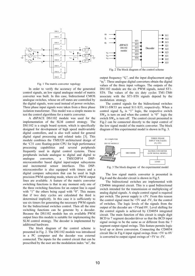
In order to verify the accuracy of the generated control signals, an low signal analogue model of matrix converter was built. In this case, bidirectional CMOS analogue switches, whose on off states are controlled by the digital signals, were used instead of power switches. Three phase input signals were taken from a three phase isolation transformer. This model was a simple means to test the control algorithms for a matrix converter.

A dSPACE DS1102 module was used for the implementation of the SLM control strategy. The DS1102 is a single board system, which is specifically designed for development of high speed multivariable digital controllers, and is also well suited for general digital signal processing and related tasks [3]. This module combines the TMS320 architectural design of the ‘C31 core floating-point CPU for high performance processing capabilities and several peripherals frequently used in digital control systems. These peripherals include analogue to digital and digital to analogue converters, a TMS320P14 DSP-microcontroller based digital input/output subsystems and incremental sensor interfaces. This DSP-microcontroller is also equipped with timers and a digital compare subsystem that can be used in high precision PWM operating mode, where six PWM output lines are available. A feature of the matrix converter switching functions is that in any moment only one of the three switching functions for an output line is equal with “1” the others being equal with “0”. This means that if two duty cycles are calculated the third is determined implicitly. In this case it is sufficiently to use six timers for generating the necessary PWM signals for the bidirectional switches control. Then all the nine switching functions can be generate by a decoder. Because the DS1102 module has six available PWM output lines this module is suitable for implementing the SLM control strategy. The decoder is implemented by additional hardware.

The block diagram of the control scheme is presented in Fig. 2. The DS1102 module was introduced in a PC computer and the decoder was external connected. The inputs for the control circuit that can be prescribed by the user are the modulation index “m”, the

output frequency “f0”, and the input displacement angle “ϕI”. Three analogue digital converters obtain the digital values of the three input voltages. The outputs of the DS1102 module are the six PWM signals, noted ST1-ST6. The values of the six duty cycles TM1-TM6 associate with the ST1-ST6 signals depend by the modulation strategy.

The control signals for the bidirectional switches SW11-SW33 are noted S11-S33, respectively. When a control signal Sjk is “1” logic, the respective switch SWjk is turn on and when the control is “0” logic the switch SWjk is turn off. The control circuit presented in Fig.2 can be connected directly to the input control of the low signal model of the matrix converter. The block diagram of this experimental model is shown in Fig. 3.

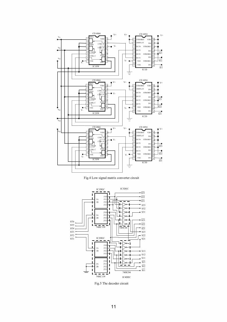
The low signal matrix converter is presented in Fig.4 and the decoder circuit is shown in Fig.5.

The bidirectional switches are implemented with CD4066 integrated circuit. This is a quad bidirectional switch intended for the transmission or multiplexing of analog digital signals. A single control signal is required per switch. The power supply is ±5V. From this reason the control signal must be +5V and -5V, for the control of switches. The logic levels of the signals from the output of the decoder are +5Vand 0V. Level shifting for the control signals is achieved by CD4054 integrated circuit. The main function of this circuit is single digit BCD to 7 segment decoder/driver so that the BCD input signal swings to be the same as or different from the 7 segment output signal swings. This feature permits logic level up or down conversion. Connecting the CD4054 circuit like in Fig.4 input signal swings from +5V to 0V is converted to output signal swings of +5V to -5V.

Fig. 1 The matrix converter topology

vI1

iI3

iI2

iI1

vI2

vI3vI31

vI23

vI12

v023

v012

v031

i01vF01

i02

i03

vF03

vF02

Z2

Z1

Z3

SW11

SW12

SW13

SW21

SW22

SW23

SW31

SW32

SW33

Fig. 2 The block diagram of the control scheme

dSPACEDS1102module

Decoder

S11S12S13

S22S21

S31S23

S32S33

ST1ST2ST3ST4

mf0

ϕI

vI1vI2vI3

ST5ST6

Fig. 3 The block diagram of the experimental model

DECODER

LOAD

MATRIX CONVERTER(LOW SIGNAL MODEL)

PC COMPUTER+

DS1102 MODULE

THREE PHASEINPUT VOLTAGES

(VI=2V)

10

13S

12S

11S

1

2

3 4

5

6 7

14

13

12 11

10

9 8

1

2

3 4

5

6 7

14

13

12 11

10

9 8

1

2

3 4

5

6 7

14

13

12 11

10

9 8

1

2

3 4

5

6 7

14

1312

11

10

9 8

15

16

1

2

3 4

5

6 7

14

1312

11

10

9 8

15

16

1

2

3 4

5

6 7

14

1312

11

10

9 8

15

16

23S

22S

21S

33S

32S

31S

vI1

vI2

vI3

v01

v02

v03

V+ V+ V+

V- V-

V-

IN1

IN2

IN3

STROBE3

STROBE1

STROBE2

IN4

OUT1

OUT2

OUT3

OUT4

VSS

VEE

STROBE4 VDD

DISPLAY

IN1

IN2

IN3

STROBE3

STROBE1

STROBE2

IN4

OUT1

OUT2

OUT3

OUT4

VSS

VEE

STROBE4 VDD

DISPLAY

IN1

IN2

IN3

STROBE3

STROBE1

STROBE2

IN4

OUT1

OUT2

OUT3

OUT4

VSS

VEE

STROBE4 VDD

DISPLAY

V+ V+ V+

V-

V+ V+ V+

V-

V- V-

V- V-

VSS

VDD

CTRL B

CTRL C

CTRL A

CTRL D

SWA

SWB

SWC

SWD

VSS

VDD

CTRL B

CTRL C

CTRL A

CTRL D

SWA

SWB

SWC

SWD

VSS

VDD

CTRL B

CTRL C

CTRL A

CTRL D

SWA

SWB

SWC

SWD

IC1D IC1SW

IC2D IC2SW

IC3D IC3SW

CD 4066 CD 4054

CD 4066 CD 4054

CD 4066 CD 4054

Fig.4 Low signal matrix converter circuit

1A 1B

1Y11Y21Y3

1Y0

2A 2B

2Y12Y22Y3

2Y0

IC1DEC

74HC139

1A 1B

1Y11Y21Y3

1Y0

2A 2B

2Y12Y22Y3

2Y0

IC2DEC

74HC139 IC4DEC

74HC04

IC3DEC

74HC04

13S

12S

11S

23S

22S

21S

33S

32S

31S

S33 S32 S31

S23 S22 S21

S13 S12 S11

ST6 ST5 ST4 ST3 ST2 ST1

Fig.5 The decoder circuit

11

Because the DSP modulator generates only six logic signal, and nine control pulses are needed for a matrix converter, in retrieve three 2 to 4 bits decoders are used, one for each phase. Additionally each output control is inverted so that the matrix converter can be controlled in “positive” logic or in “negative” logic.

III. EXPERIMENTAL RESULTS

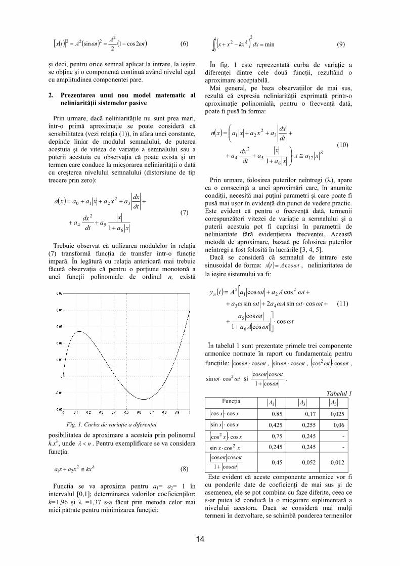
In order to verify the feasibility of the proposed low signal model the matrix converter was controlled by means of the SLM modulation strategy. This control algorithm was proposed first in [4] and [5] by the authors of these papers. A detailed analyses of the SLM control strategy is presented in [6]. The main advantages of this strategy are: immediate comprehension of the required commutation processes, simplified control algorithm and maximum voltage transfer without adding third harmonic components. In Fig.6 is presented the theoretical output line to line voltage waveform in a PWM period.

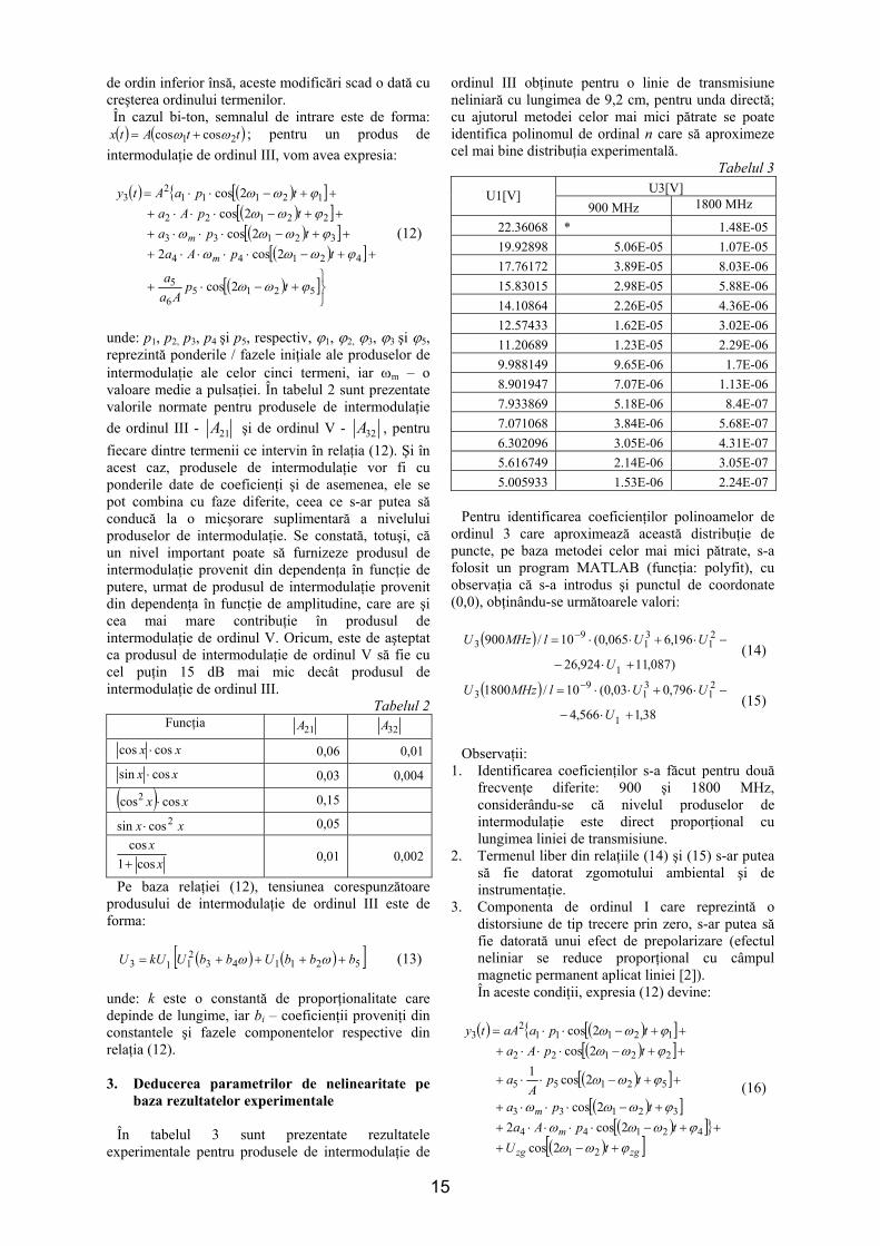
In Fig.7 is shown a detail of the experimental line to line voltage waveform obtained at the output of the low signal model, presented in Fig.4.

It is observed that experimental voltage waveform is close by the theoretical waveform.

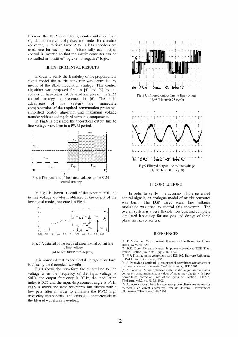
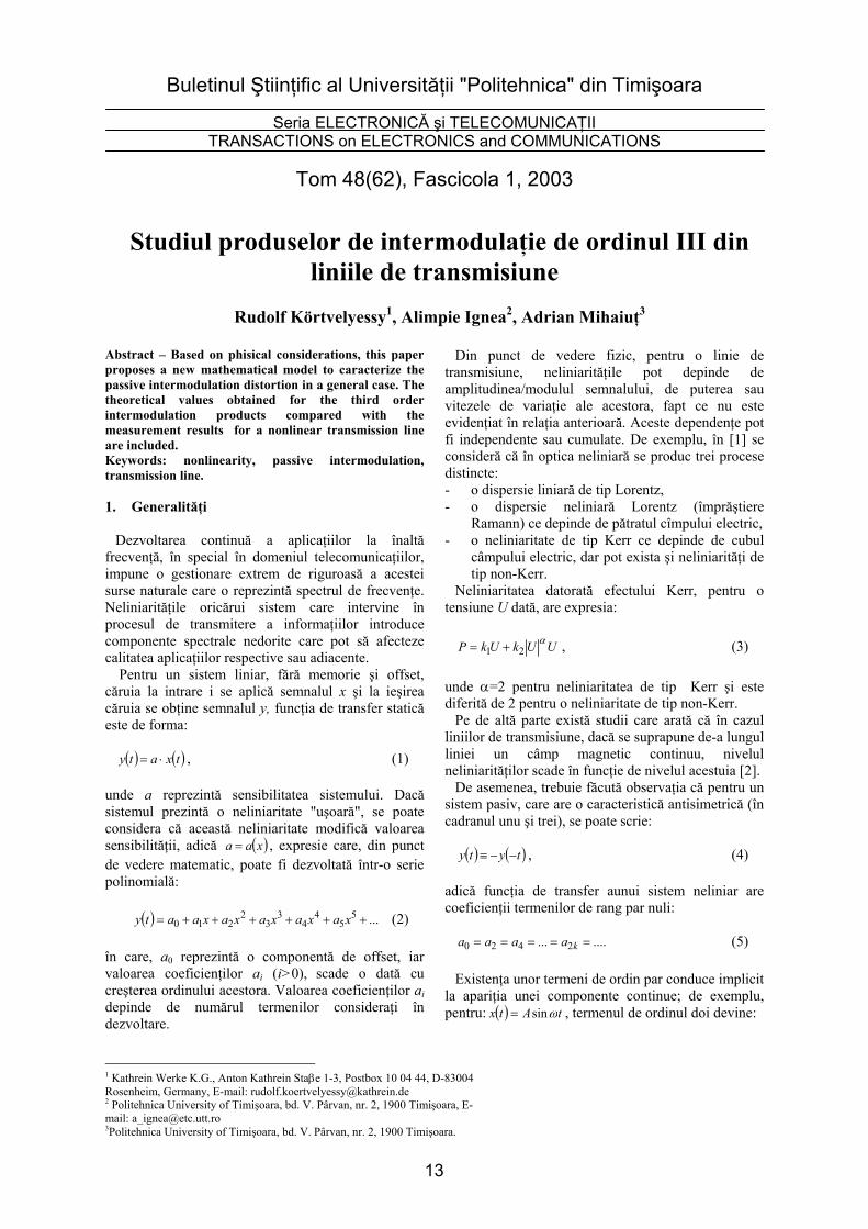
Fig.8 shows the waveform the output line to line voltage when the frequency of the input voltage is 50Hz, the output frequency is 80Hz, the modulation index is 0.75 and the input displacement angle is 0º. In Fig.9 is shown the same waveform, but filtered with a low pass filter in order to eliminate the PWM high frequency components. The sinusoidal characteristic of the filtered waveform is evident.

II. CONCLUSIONS

In order to verify the accuracy of the generated

control signals, an analogue model of matrix converter was built.. The DSP based scalar line voltages modulator was used to control this converter. The overall system is a very flexible, low cost and complete simulated laboratory for analysis and design of three phase matrix converters.

REFERENCES [1] R. Valentine; Motor control. Electronics Handbook; Mc Graw-Hill, New York; 1998 [2] B.K. Bose; Recent advances in power electronics; IEEE Tran. Power Electron., vol.7, no.1, pg. 2-16; 1992 [3] ***; Floating-point controller board DS1102, Harware Reference; dSPACE GmbH,Germany; 1999 [4] A. Popovici; Contribuţii la cercetarea şi dezvoltarea convertoarelor matriceale de curent alternativ; Teză de doctorat, UPT, 2002 [5] A. Popovici; A new optimised scalar control algorithm for matrix converters using instantaneous values of input line voltages with input power factor correction; Proc. of the Symp. on Electron., "Etc'98", Timişoara, vol.2, pg. 68-73; 1998 [6] A.Popovici; Contribuţii la cercetarea şi dezvoltarea convertoarelor matriceale de curent alternativ; Teză de doctorat; Universitatea „Politehnica” Timişoara, iulie 2002.

Fig. 6 The synthesis of the output voltage for the SLM control strategy

v0pq

vIaa

vIab

-vIca

TS

Tpqa Tpqc Tpqb

Fig. 7 A detailed of the acquired experimental output line to line voltage

(SLM f0=100Hz m=0.8 ϕI=0)

0.15 0.2 0.25 0.3 0.35 0.4 0.45 0.5 0.55 0.6 0.650

2

4

6

8

10TS

Tpqa Tpqc Tpqb

vIaa-vIca vIab

Fig.8 Unfiltered output line to line voltage ( f0=80Hz m=0.75 ϕI=0)

Fig.9 Filtered output line to line voltage ( f0=80Hz m=0.75 ϕI=0)

12

Buletinul Ştiinţific al Universităţii "Politehnica" din Timişoara

Seria ELECTRONICĂ şi TELECOMUNICAŢII TRANSACTIONS on ELECTRONICS and COMMUNICATIONS

Tom 48(62), Fascicola 1, 2003

Studiul produselor de intermodulaţie de ordinul III din liniile de transmisiune

Rudolf Körtvelyessy1, Alimpie Ignea2, Adrian Mihaiuţ3

1 Kathrein Werke K.G., Anton Kathrein Staβe 1-3, Postbox 10 04 44, D-83004 Rosenheim, Germany, E-mail: rudolf.koertvelyessy@kathrein.de 2 Politehnica University of Timişoara, bd. V. Pârvan, nr. 2, 1900 Timişoara, E-mail: a_ignea@etc.utt.ro 3Politehnica University of Timişoara, bd. V. Pârvan, nr. 2, 1900 Timişoara.

Abstract – Based on phisical considerations, this paper proposes a new mathematical model to caracterize the passive intermodulation distortion in a general case. The theoretical values obtained for the third order intermodulation products compared with the measurement results for a nonlinear transmission line are included. Keywords: nonlinearity, passive intermodulation, transmission line. 1. Generalităţi

Dezvoltarea continuă a aplicaţiilor la înaltă frecvenţă, în special în domeniul telecomunicaţiilor, impune o gestionare extrem de riguroasă a acestei surse naturale care o reprezintă spectrul de frecvenţe. Neliniarităţile oricărui sistem care intervine în procesul de transmitere a informaţiilor introduce componente spectrale nedorite care pot să afecteze calitatea aplicaţiilor respective sau adiacente.

Pentru un sistem liniar, fără memorie şi offset, căruia la intrare i se aplică semnalul x şi la ieşirea căruia se obţine semnalul y, funcţia de transfer statică este de forma:

( ) ( )txaty ⋅= , (1)

unde a reprezintă sensibilitatea sistemului. Dacă sistemul prezintă o neliniaritate "uşoară", se poate considera că această neliniaritate modifică valoarea sensibilităţii, adică ( )xaa = , expresie care, din punct de vedere matematic, poate fi dezvoltată într-o serie polinomială:

( ) ...55

44

33

2210 ++++++= xaxaxaxaxaaty (2)

în care, a0 reprezintă o componentă de offset, iar valoarea coeficienţilor ai (i>0), scade o dată cu creşterea ordinului acestora. Valoarea coeficienţilor ai depinde de numărul termenilor consideraţi în dezvoltare.

Din punct de vedere fizic, pentru o linie de transmisiune, neliniarităţile pot depinde de amplitudinea/modulul semnalului, de puterea sau vitezele de variaţie ale acestora, fapt ce nu este evidenţiat în relaţia anterioară. Aceste dependenţe pot fi independente sau cumulate. De exemplu, în [1] se consideră că în optica neliniară se produc trei procese distincte: - o dispersie liniară de tip Lorentz, - o dispersie neliniară Lorentz (împrăştiere

Ramann) ce depinde de pătratul cîmpului electric, - o neliniaritate de tip Kerr ce depinde de cubul

câmpului electric, dar pot exista şi neliniarităţi de tip non-Kerr.

Neliniaritatea datorată efectului Kerr, pentru o tensiune U dată, are expresia:

UUkUkP α

21 += , (3) unde α=2 pentru neliniaritatea de tip Kerr şi este diferită de 2 pentru o neliniaritate de tip non-Kerr.

Pe de altă parte există studii care arată că în cazul liniilor de transmisiune, dacă se suprapune de-a lungul liniei un câmp magnetic continuu, nivelul neliniarităţilor scade în funcţie de nivelul acestuia [2].

De asemenea, trebuie făcută observaţia că pentru un sistem pasiv, care are o caracteristică antisimetrică (în cadranul unu şi trei), se poate scrie:

( ) ( )tyty −−≡ , (4)

adică funcţia de transfer aunui sistem neliniar are coeficienţii termenilor de rang par nuli:

....... 2420 ===== kaaaa (5) Existenţa unor termeni de ordin par conduce implicit

la apariţia unei componente continue; de exemplu, pentru: ( ) tAtx ωsin= , termenul de ordinul doi devine:

13

( )[ ] ( ) ( )tAtAtx ωω 2cos12

sin2

222 −== (6)

şi deci, pentru orice semnal aplicat la intrare, la ieşire se obţine şi o componentă continuă având nivelul egal cu amplitudinea componentei pare. 2. Prezentarea unui nou model matematic al

neliniarităţii sistemelor pasive

Prin urmare, dacă neliniarităţile nu sunt prea mari, într-o primă aproximaţie se poate consideră că sensibilitatea (vezi relaţia (1)), în afara unei constante, depinde liniar de modulul semnalului, de puterea acestuia şi de viteza de variaţie a semnalului sau a puterii acestuia cu observaţia că poate exista şi un termen care conduce la micşorarea neliniarităţii o dată cu creşterea nivelului semnalului (distorsiune de tip trecere prin zero):

( )

xax

adt

dxa

dtdxaxaxaaxa

65

2

4

32

210

1+++

++++=

(7)

Trebuie observat că utilizarea modulelor în relaţia

(7) transformă funcţia de transfer într-o funcţie impară. În legătură cu relaţia anterioară mai trebuie făcută observaţia că pentru o porţiune monotonă a unei funcţii polinomiale de ordinul n, există

posibilitatea de aproximare a acesteia prin polinomul k.xλ, unde n<λ . Pentru exemplificare se va considera funcţia:

λkxxaxa ≅+ 2

21 (8)

Funcţia se va aproxima pentru a1= a2= 1 în intervalul [0,1]; determinarea valorilor coeficienţilor: k=1,96 şi λ =1,37 s-a făcut prin metoda celor mai mici pătrate pentru minimizarea funcţiei:

( ) min21

0

2 =−+∫ dxkxxx λ (9)

În fig. 1 este reprezentată curba de variaţie a

diferenţei dintre cele două funcţii, rezultând o aproximare acceptabilă.

Mai general, pe baza observaţiilor de mai sus, rezultă că expresia neliniarităţii exprimată printr-o aproximaţie polinomială, pentru o frecvenţă dată, poate fi pusă în forma:

( )

λxaxxa

xa

dtdxa

dtdxaxaxaxn

126

5

2

4

32

21

1 ≅⋅⎟

⎟⎠

⎞

+++

⎜⎜⎝

⎛+++=

(10)

Prin urmare, folosirea puterilor neîntregi (λ), apare

ca o consecinţă a unei aproximări care, în anumite condiţii, necesită mai puţini parametri şi care poate fi pusă mai uşor în evidenţă din punct de vedere practic. Este evident că pentru o frecvenţă dată, termenii corespunzători vitezei de variaţie a semnalului şi a puterii acestuia pot fi cuprinşi în parametrii de neliniaritate fără evidenţierea frecvenţei. Această metodă de aproximare, bazată pe folosirea puterilor neîntregi a fost folosită în lucrările [3, 4, 5].

Dacă se consideră că semnalul de intrare este sinusoidal de forma: ( ) tAtx ωcos= , neliniaritatea de la ieşire sistemului va fi:

( ) [

ωttAa

ta

ωtωtωAaωtωa

ωtAaωtaAtyn

coscos1

cos

cossin2sin

coscos

6

5

43

221

2

⋅⎥⎥⎦

⎤

++

+⋅++

++=

ωω

(11)

În tabelul 1 sunt prezentate primele trei componente

armonice normate în raport cu fundamentala pentru funcţiile: tt ωω coscos ⋅ , tt ωω cossin ⋅ , ( ) tt ωω coscos2 ⋅ ,

tt ωω 2cossin ⋅ şi t

ttωωω

cos1coscos

+.

Tabelul 1 Funcţia 1A 3A 5A

xx coscos ⋅ 0.85 0,17 0,025

xx cossin ⋅ 0,425 0,255 0,06

( ) xx coscos2 ⋅ 0,75 0,245 -

xx 2cossin ⋅ 0,245 0,245 -

ttt

ωωω

cos1coscos

+ 0,45 0,052 0,012

Este evident că aceste componente armonice vor fi cu ponderile date de coeficienţi de mai sus şi de asemenea, ele se pot combina cu faze diferite, ceea ce s-ar putea să conducă la o micşorare suplimentară a nivelului acestora. Dacă se consideră mai mulţi termeni în dezvoltare, se schimbă ponderea termenilor

Fig. 1. Curba de variaţie a diferenţei.

14

de ordin inferior însă, aceste modificări scad o dată cu creşterea ordinului termenilor. În cazul bi-ton, semnalul de intrare este de forma: ( ) ( )ttAtx 21 coscos ωω += ; pentru un produs de

intermodulaţie de ordinul III, vom avea expresia:

( ) ( )[ ]( )[ ]( )[ ]

( )[ ]

( )[ ]⎭⎬⎫

+−⋅+

++−⋅⋅⋅⋅+++−⋅⋅⋅+++−⋅⋅⋅+

++−⋅⋅=

52156

5

42144

32133

22122

121112

3

2cos

2cos22cos

2cos2cos

ϕωω

ϕωωωϕωωω

ϕωωϕωω

tpAa

a

tpAatpa

tpAatpaAty

m

m (12)

unde: p1, p2, p3, p4 şi p5, respectiv, ϕ1, ϕ2, ϕ3, ϕ3 şi ϕ5, reprezintă ponderile / fazele iniţiale ale produselor de intermodulaţie ale celor cinci termeni, iar ωm – o valoare medie a pulsaţiei. În tabelul 2 sunt prezentate valorile normate pentru produsele de intermodulaţie de ordinul III - 21A şi de ordinul V - 32A , pentru fiecare dintre termenii ce intervin în relaţia (12). Şi în acest caz, produsele de intermodulaţie vor fi cu ponderile date de coeficienţi şi de asemenea, ele se pot combina cu faze diferite, ceea ce s-ar putea să conducă la o micşorare suplimentară a nivelului produselor de intermodulaţie. Se constată, totuşi, că un nivel important poate să furnizeze produsul de intermodulaţie provenit din dependenţa în funcţie de putere, urmat de produsul de intermodulaţie provenit din dependenţa în funcţie de amplitudine, care are şi cea mai mare contribuţie în produsul de intermodulaţie de ordinul V. Oricum, este de aşteptat ca produsul de intermodulaţie de ordinul V să fie cu cel puţin 15 dB mai mic decât produsul de intermodulaţie de ordinul III.

Tabelul 2 Funcţia 21A 32A

xx coscos ⋅ 0,06 0,01

xx cossin ⋅ 0,03 0,004

( ) xx coscos2 ⋅ 0,15

xx 2cossin ⋅ 0,05

xx

cos1cos+

0,01 0,002

Pe baza relaţiei (12), tensiunea corespunzătoare produsului de intermodulaţie de ordinul III este de forma:

( ) ( )[ ]5211432113 bbbUbbUkUU ++++= ωω (13)

unde: k este o constantă de proporţionalitate care depinde de lungime, iar bi – coeficienţii proveniţi din constantele şi fazele componentelor respective din relaţia (12). 3. Deducerea parametrilor de nelinearitate pe

baza rezultatelor experimentale

În tabelul 3 sunt prezentate rezultatele experimentale pentru produsele de intermodulaţie de

ordinul III obţinute pentru o linie de transmisiune neliniară cu lungimea de 9,2 cm, pentru unda directă; cu ajutorul metodei celor mai mici pătrate se poate identifica polinomul de ordinal n care să aproximeze cel mai bine distribuţia experimentală.

Tabelul 3 U3[V] U1[V]

900 MHz 1800 MHz

22.36068 * 1.48E-05 19.92898 5.06E-05 1.07E-05 17.76172 3.89E-05 8.03E-06 15.83015 2.98E-05 5.88E-06 14.10864 2.26E-05 4.36E-06 12.57433 1.62E-05 3.02E-06 11.20689 1.23E-05 2.29E-06 9.988149 9.65E-06 1.7E-06 8.901947 7.07E-06 1.13E-06 7.933869 5.18E-06 8.4E-07 7.071068 3.84E-06 5.68E-07 6.302096 3.05E-06 4.31E-07 5.616749 2.14E-06 3.05E-07 5.005933 1.53E-06 2.24E-07

Pentru identificarea coeficienţilor polinoamelor de

ordinul 3 care aproximează această distribuţie de puncte, pe baza metodei celor mai mici pătrate, s-a folosit un program MATLAB (funcţia: polyfit), cu observaţia că s-a introdus şi punctul de coordonate (0,0), obţinându-se următoarele valori:

( ))087,11924,26

196,6065,0(10/900

1

21

31

93

+⋅−

−⋅+⋅⋅= −

U

UUlMHzU (14)

( )38,1566,4

796,003,0(10/1800

1

21

31

93

+⋅−

−⋅+⋅⋅= −

U

UUlMHzU (15)

Observaţii:

1. Identificarea coeficienţilor s-a făcut pentru două frecvenţe diferite: 900 şi 1800 MHz, considerându-se că nivelul produselor de intermodulaţie este direct proporţional cu lungimea liniei de transmisiune.

2. Termenul liber din relaţiile (14) şi (15) s-ar putea să fie datorat zgomotului ambiental şi de instrumentaţie.

3. Componenta de ordinul I care reprezintă o distorsiune de tip trecere prin zero, s-ar putea să fie datorată unui efect de prepolarizare (efectul neliniar se reduce proporţional cu câmpul magnetic permanent aplicat liniei [2]). În aceste condiţii, expresia (12) devine: ( ) ( )[ ]

( )[ ]( )[ ]( )[ ]

( )[ ]( )[ ]zgzg

m

m

tUtpAa

tpa

tpA

a

tpAatpaaAty

ϕωωϕωωω

ϕωωω

ϕωω

ϕωωϕωω

+−+

++−⋅⋅⋅⋅++−⋅⋅⋅+

++−⋅⋅+

++−⋅⋅⋅+++−⋅⋅=

21

42144

32133

52155

22122

121112

3

2cos2cos2

2cos

2cos12cos2cos

(16)

15

sau:

( ) ( )( ) 0651

432121

31

0112213

313 /

abbU

bbUbbU

aaUaUaUlU

+⋅+⋅+

+⋅+⋅+⋅+⋅=

=+⋅+⋅+⋅=

ω

ωω (17)

Relaţia (17) indică faptul că, dacă dispunem de

rezultate experimentale pentru două frecvenţe diferite se pot determina coeficienţii bi prin formarea sistemelor de ecuaţii:

( )( )213221

13121

ωωωω

abbabb

=⋅+

=⋅+ (18.a)

( )( )212243

12143

ωωωω

abbabb

=⋅+=⋅+

(18.b)

( )( )211265

11165

ωωωω

abbabb

=⋅+=⋅+

(18.c)

Rezolvând sistemele (18) se obţine:

( )[

( )( ) ]42.15025,083.46

0064,008,12

000028,0086,010/

1

21

31

93

−⋅−⋅−

−⋅−⋅+

+⋅−⋅⋅= −

ω

ω

ω

U

U

UlU (19)

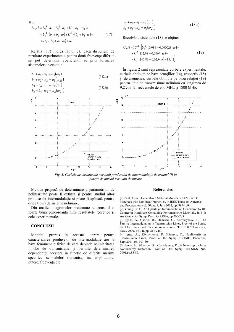
În figura 2 sunt reprezentate curbele experimentale,

curbele obţinute pe baza ecuaţiilor (14), respectiv (15) şi de asemenea, curbele obţinute pe baza relaţiei (19) pentru linia de transmisiune neliniară cu lungimea de 9,2 cm, la frecvenţele de 900 MHz şi 1800 MHz.

Metoda propusă de determinare a parametrilor de

neliniaritate poate fi extinsă şi pentru studiul altor produse de intermodulaţie şi poate fi aplicată pentru orice tipuri de sisteme neliniare.

Din analiza diagramelor prezentate se constată o foarte bună concordanţă între rezultatele teoretice şi cele experimentale.

CONCLUZII

Modelul propus în această lucrare pentru

caracterizarea produselor de intermodulaţie are la bază fenomenele fizice de care depinde neliniaritatea liniilor de transmisiune şi permite determinarea dependenţei acestora în funcţie de diferite mărimi specifice semnalelor transmise, ca amplitudine, putere, frecvenţă etc.

Referencies

[1] Paul, J. ş.a. Generalized Material Models in TLM-Part 3: Materials with Nonlinear Properties, în IEEE Trans. on Antennas and Propagation, vol. 50, nr. 7, July 2002, pp. 997-1004 [2] Young, Ch.E., An Update on Intermodulation Generation by RF Connector Hardware Containing Ferromagnetic Materials, in 9-th An. Connector Symp. Proc., Oct.1976, pp.266-283 [3] Ignea, A., Gabriel, R., Stănescu, O., Körtvelyessy, R., The Passive Intermodulation in Transmission Lines, Proc. of the Symp. on Electronics and Telecommunications "ETc.2000",Timisoara, Nov., 2000, Vol. II, pp. 211-215. [4] Ignea, A.., Körtvelyessy, R. Stănescu, O., Nonlinearity in Transmission Lines, Proc. of the Symp. SIITME, Bucureşti, Sept.2001, pp. 301-304 [5] Ignea, A., Stănescu, O., Körtvelyessy, R., A New approach on Nonlinearity Distortion, Proc. of Int. Symp. TELSIKS, Nis, 2001,pp.83-87.

Fig. 3. Curbele de variaţie ale tensiunii produsului de intermodulaţie de ordinul III în funcţie de nivelul tensiunii de intrare

16

Buletinul Ştiinţific al Universităţii "Politehnica" din Timişoara

Seria ELECTRONICĂ şi TELECOMUNICAŢII TRANSACTIONS on ELECTRONICS and COMMUNICATIONS

Tom 48(62), Fascicola 1, 2003

Accurate Harmonics Analyzer

Daniel Belega 1 and Dan Stoiciu1

1 Dept. of Measurements and Optical Electronics, Faculty of Electronics and Telecommunications, e-mail: belega@etc.utt.ro, dstoiciu@etc.utt.ro.

Abstract – This paper presents the operating principles and the main characteristics of a harmonics analyzer. This analyzer provides the statistical performance of the total harmonic distortion (THD) and of the amplitudes of the fundamental and of the first 15 harmonic components of a periodical signal. The amplitudes of the harmonic components were measured with high accuracy by the algorithm proposed in reference [1] and by interpolated fast Fourier transform (Interpolated FFT) algorithm. The available graphical pages with their information and facilities are thoroughly illustrated in some practical applications. Keywords: estimation of the harmonic components, total harmonic distortion, DFT, Interpolated FFT algorithm.

I. INTRODUCTION In modern measurement and control applications there is often need to determine with high accuracy the amplitudes of the harmonic components of a periodical signal. Based upon these components the total harmonic distortion (THD) of the signal can be calculated. The amplitudes of the harmonic components are mostly estimated by frequency-domain analysis [1], [2], [3]. In frequency-domain analysis the signal under test is applied to a digitizing waveform recorder that must have better performances than the ones of the signal analyzed. Then a certain algorithm, based on discrete Fourier transform (DFT) of the digitized data sequence, is employed to estimate the amplitudes of the harmonic components. The most precise and thus widely used algorithms for estimating the amplitudes of harmonic components of a periodical signal when the sampling process is noncoherent with the signal analyzed are the algorithm proposed in [1] and the interpolated fast Fourier transform (Interpolated FFT) algorithm [2]. In this paper an accurate harmonics analyzer is presented. This analyzer determines the statistical performance (mean and standard deviation) of the THD and of the amplitudes of the fundamental and of the first 15 harmonic components of the signal under test. The statistical analysis is made because this kind of analysis provides more important and realistic information than a non-statistical one. The harmonic

components are estimated by the algorithm proposed in [1] and by the Interpolated FFT algorithm.

II. ESTIMATION OF AMPLITUDES OF HARMONIC COMPONENTS AND OF THD OF A

PERIODIC SIGNAL The signal analyzed y(t) has the frequency fin (unknown). This signal is discretized by means of a digitizing waveform recorder. The discrete-time signal obtained is y(mTs), m = 0, 1,…, M-1, where Ts = 1/fs is the digitizer sampling period and M is the number of samples acquired. In practical applications frequently the sampling process is noncoherent with the signal under test. In this case the relationship between the frequencies fin and fs is

MMJ

MJ

ff

s

in δ+=

δ+=

(1)

where J is the number of cycles of the signal under test (J is an integer) and 0 < δ < 1. In the case of noncoherent sampling spectral leakage arises. The leakage errors are reduced by windowing. This produces the sequence yw(mTs) = y(mTs)w(mTs), m = 0, 1,…,M-1, where w(mTs) is the window function. Generally a Blackman-Harris window type with H coefficients is used. The spectrum Yw(l), l = 0, 1,…, M-1, of yw(mTs) is obtained by means of the DFT. The maximum values of the modulus |Yw(l)| occur for the index values K and, symmetrically, for M-K. The maximum values of ith harmonic component (i ≥ 2) occur for the index value li, and, symmetrically, for M- li. The amplitudes of the fundamental and of the harmonic component i (i = 2, 3, …, 15) and THD were estimated by the algorithm proposed in [1] and by the Interpolated FFT algorithm [2]. Based on the algorithm proposed in [1] the amplitude of the fundamental A1est1 and of the harmonic component i (i =2, 3, …, 15) Aiest1 were estimated by the expressions:

17

( )

( )

( )∑

∑

∑

−

=

+

−=

+

−=

=

−=

=

=

1

0

2

221

2211

1

,1,,1,0

,4

,4

M

l

Hil

Hillwiest

HK

HKlwest

lwM

NNPG

Mi

lYNNPGM

A

lYNNPGM

A

K

(2)

where NNPG is the normalized noise power gain. With the algorithm proposed in [1] THD was estimated by

( )

( ) ( ).lg10

][

15

2

22

15

2

2

1

⎟⎟⎟⎟⎟⎟

⎠

⎞

⎜⎜⎜⎜⎜⎜

⎝

⎛

+

=

∑ ∑∑

∑ ∑

=

+

−=

+

−=

=

+

−=

i

Hl

Hllw

HK

HKlw

i

Hl

Hllw

est

i

i

i

i

lYlY

lY

dBcTHD

(3)

The Interpolated FFT algorithm estimates THD by

∑=

⎟⎟⎠

⎞⎜⎜⎝

⎛

+

=15

22

22

21

22

2

lg10

][

i iestest

iest

est

AAA

dBcTHD

(4)

where A1est2 is the amplitude of the fundamental estimated by the Interpolated FFT algorithm; Aiest2 is the amplitude of the harmonic component i (i = 2, 3, …, 15) estimated by the Interpolated FFT algorithm.

III. PRESENTATION OF THE HARMONICS ANALYZER

The harmonics analyzer has the following key features: • The acquisition system is based on a TMS320C5x DSK board [4]. • The data is collected as a series of R records, each of M samples (256 ≤ M ≤ 4096). • The software used is easy to use; it interacts with the user through mouse driven graphic interfaces. • Estimation of THD. • Estimation of the amplitudes of the fundamental and of the first 15 harmonic components. • Two algorithms were employed to estimate THD and the amplitudes of the fundamental and of the harmonic components: - algorithm proposed in [1]; - Interpolated FFT algorithm [2].

• Compute the statistical performances of the THD and of the amplitudes of fundamental and harmonic components. • An output graphical page is available for THD, fundamental and each harmonic component. • Possibility to process also data files obtained by simulation or by means of another acquisition system. The block diagram of the harmonic analyzer is presented in Fig. 1.

Fig.1. Block diagram of the harmonics analyzer. The TMS320C5x DSK is a low-cost, simple, stand-alone application board equipped with a 16-bit fixed-point digital signal processor (DSP) TMS320C50. The DSK contains an analog interface circuit (AIC) - TLC32040, which provides the necessary conversion between the analogue and digital domain. For this purpose the TLC32040 incorporates a band-pass antialiasing input filter, a 14-bit analog-to-digital converter (ADC), a serial port by which the AIC communicates with the TMS320C50, a 14-bit digital-to-analog converter (DAC) and a low-pass output reconstruction filter. The DSK is connected to a PC via a RS232 interface. The maximum sampling frequency of the DSK is 50 kHz. The data processing and the interactive graphical pages were realized in MATLAB 4.2.

IV. SOME EXPERIMETAL RESULTS In order to reveal the features offered by the harmonics analyzer some experiments were carried out. First, a bipolar square wave generated by the programmable function generator HM8130 was analyzed. The square wave was characterized by 1.28 kHz frequency, 2 V amplitude, 0 V offset and 50% duty cycle. The DSK board has been set to: sampling frequency fs = 15.625 kHz, the gain of the preamplifier - 2 (for which the full scale range (FSR) of the ADC of the AIC is 6 V) and without the input band-pass filter of the AIC. A number of R = 60 records with M = 1048 samples per record was acquired. The 4-term minimum error energy window was used [5]. The statistical performances concerning the harmonic contents of the square wave obtained with the harmonics analyzer are given in Table I.

Acquisition system (TMS320C5x DSK)

PC (signal

processing)

RS232C

Signal analyzed

18

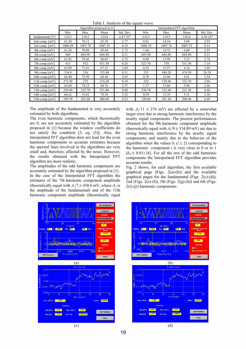
Table I. Analysis of the square wave. Algorithm proposed in [1] Interpolated FFT algorithm

Min. Max. Mean Std. Dev. Min. Max. Mean Std. Dev. fundamental [V] 3.013 3.015 3.014 4.47·10-4 3.013 3.015 3.014 4.50·10-4

2nd comp. [mV] 61.20 70.12 65.39 2.77 0.81 14.54 5.09 2.93 3rd comp. [mV] 1006.69 1007.78 1007.39 0.19 1006.76 1007.76 1007.33 0.23 4th comp [mV] 61.26 70.08 65.44 2.72 1.66 14.72 6.60 2.55 5th comp [mV] 604 604.90 604.40 0.21 603.90 604.80 604.40 0.21 6th comp [mV] 61.82 70.66 66.03 2.72 0.40 13.98 5.23 2.76 7th comp [mV] 431 432 431.50 0.26 523.70 538 531.30 3.14 8th comp [mV] 63.09 71.81 67.21 2.69 0.52 15.37 4.16 3.45 9th comp [mV] 334.8 336 335.40 0.31 335 484.20 474.50 26.24 10th comp [mV] 64.40 72.99 68.44 2.65 0.70 12.06 4.01 2.54 11th comp [mV] 273.50 275 274.20 0.39 325 339.40 332.70 2.96 12th comp [mV] 65.84 74.15 69.76 2.57 1.37 13.86 5.96 2.46 13th comp [mV] 230.90 232.70 231.80 0.48 230.70 232.40 231.50 0.46 14th comp [mV] 66.62 74.82 70.54 2.52 0.59 13.39 5.31 2.56 15th comp [mV] 199.70 201.60 200.60 0.53 199.60 201.30 200.40 0.49

The amplitude of the fundamental is very accurately estimated by both algorithms. The even harmonic components, which theoretically are 0, are not accurately estimated by the algorithm proposed in [1] because the window coefficients do not satisfy the condition [3, eq. (5)]. Also, the Interpolated FFT algorithm does not lead for the even harmonic components to accurate estimates because the spectral lines involved in the algorithms are very small and, therefore, affected by the noise. However, the results obtained with the Interpolated FFT algorithm are more realistic. The amplitudes of the odd harmonic components are accurately estimated by the algorithm proposed in [1]. In the case of the Interpolated FFT algorithm the estimates of the 7th harmonic component amplitude (theoretically equal with A1/7 ≅ 430.6 mV, where A1 is the amplitude of the fundamental) and of the 11th harmonic component amplitude (theoretically equal

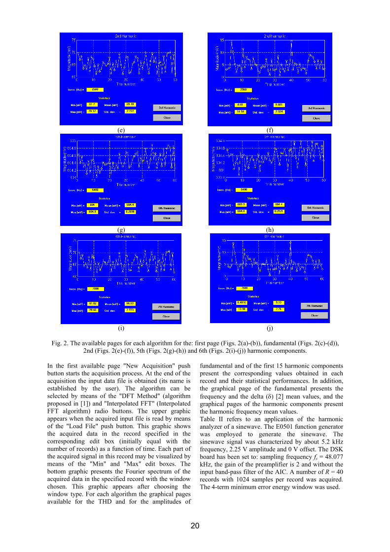
with A1/11 ≅ 274 mV) are affected by a somewhat larger error due to strong harmonic interference by the nearby signal components. The poorest performances obtained for the 9th harmonic component amplitude (theoretically equal with A1/9 ≅ 334.89 mV) are due to strong harmonic interference by the nearby signal components, and mainly due to the behavior of the algorithm when the values δi (i ≥ 2) corresponding to the harmonic component i is very close to 0 or to 1 (δ9 ≅ 0.01) [6]. For all the rest of the odd harmonic components the Interpolated FFT algorithm provides accurate results. Fig. 2 shows, for each algorithm, the first available graphical page (Figs. 2(a)-(b)) and the available graphical pages for the fundamental (Figs. 2(c)-(d)), 2nd (Figs. 2(e)-(f)), 5th (Figs. 2(g)-(h)) and 6th (Figs. 2(i)-(j)) harmonic components.

(a) (b)

(c) (d)

19

(e) (f)

(g) (h)

(i) (j)

Fig. 2. The available pages for each algorithm for the: first page (Figs. 2(a)-(b)), fundamental (Figs. 2(c)-(d)),

2nd (Figs. 2(e)-(f)), 5th (Figs. 2(g)-(h)) and 6th (Figs. 2(i)-(j)) harmonic components. In the first available page "New Acquisition" push button starts the acquisition process. At the end of the acquisition the input data file is obtained (its name is established by the user). The algorithm can be selected by means of the "DFT Method" (algorithm proposed in [1]) and "Interpolated FFT" (Interpolated FFT algorithm) radio buttons. The upper graphic appears when the acquired input file is read by means of the "Load File" push button. This graphic shows the acquired data in the record specified in the corresponding edit box (initially equal with the number of records) as a function of time. Each part of the acquired signal in this record may be visualized by means of the "Min" and "Max" edit boxes. The bottom graphic presents the Fourier spectrum of the acquired data in the specified record with the window chosen. This graphic appears after choosing the window type. For each algorithm the graphical pages available for the THD and for the amplitudes of

fundamental and of the first 15 harmonic components present the corresponding values obtained in each record and their statistical performances. In addition, the graphical page of the fundamental presents the frequency and the delta (δ) [2] mean values, and the graphical pages of the harmonic components present the harmonic frequency mean values. Table II refers to an application of the harmonic analyzer of a sinewave. The E0501 function generator was employed to generate the sinewave. The sinewave signal was characterized by about 5.2 kHz frequency, 2.25 V amplitude and 0 V offset. The DSK board has been set to: sampling frequency fs = 48.077 kHz, the gain of the preamplifier is 2 and without the input band-pass filter of the AIC. A number of R = 40 records with 1024 samples per record was acquired. The 4-term minimum error energy window was used.

20

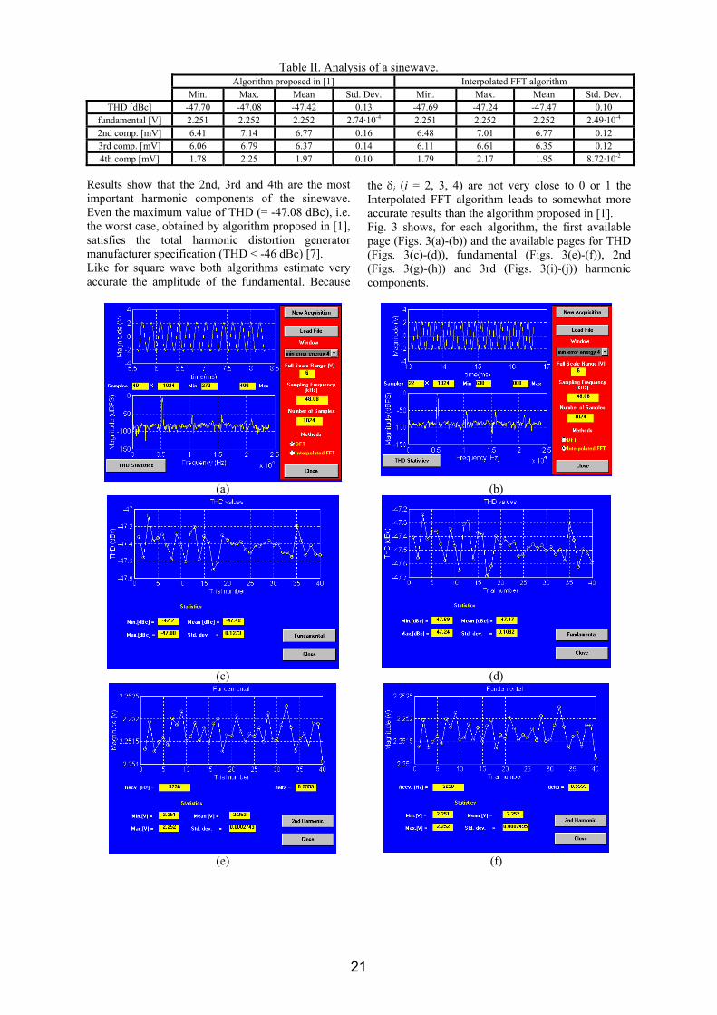
Table II. Analysis of a sinewave. Algorithm proposed in [1] Interpolated FFT algorithm

Min. Max. Mean Std. Dev. Min. Max. Mean Std. Dev. THD [dBc] -47.70 -47.08 -47.42 0.13 -47.69 -47.24 -47.47 0.10

fundamental [V] 2.251 2.252 2.252 2.74·10-4 2.251 2.252 2.252 2.49·10-4

2nd comp. [mV] 6.41 7.14 6.77 0.16 6.48 7.01 6.77 0.12 3rd comp. [mV] 6.06 6.79 6.37 0.14 6.11 6.61 6.35 0.12 4th comp [mV] 1.78 2.25 1.97 0.10 1.79 2.17 1.95 8.72·10-2

Results show that the 2nd, 3rd and 4th are the most important harmonic components of the sinewave. Even the maximum value of THD (= -47.08 dBc), i.e. the worst case, obtained by algorithm proposed in [1], satisfies the total harmonic distortion generator manufacturer specification (THD < -46 dBc) [7]. Like for square wave both algorithms estimate very accurate the amplitude of the fundamental. Because

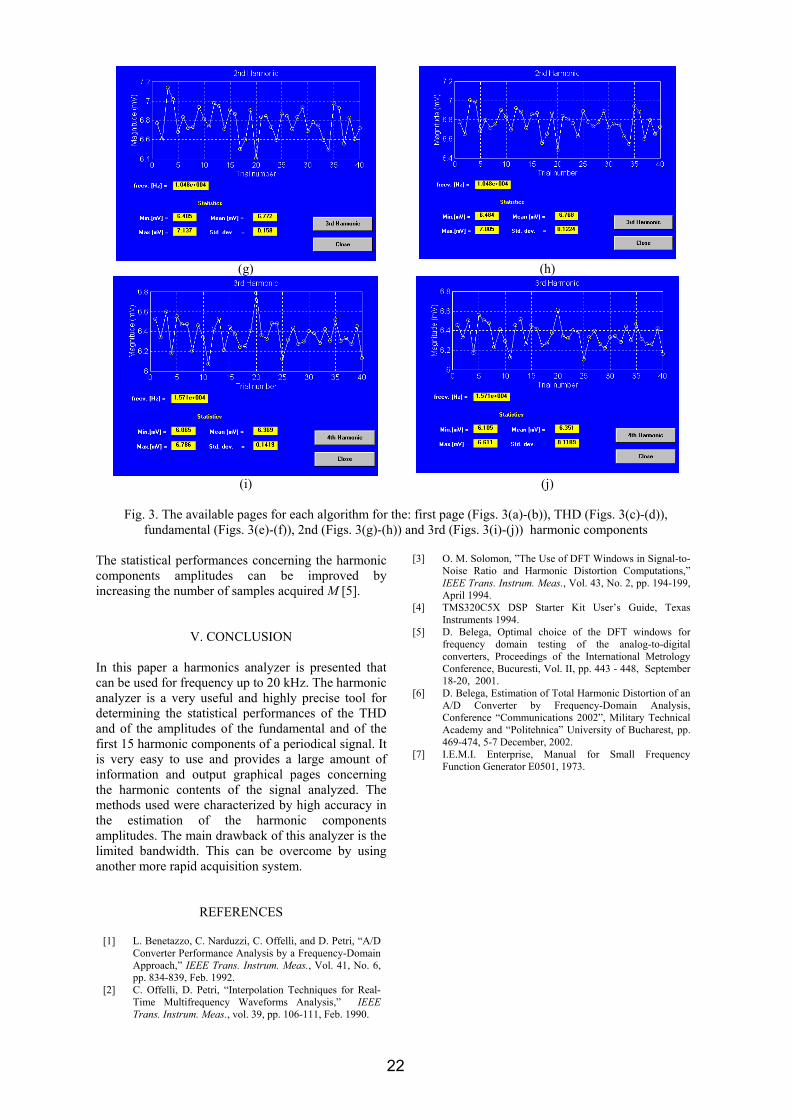
the δi (i = 2, 3, 4) are not very close to 0 or 1 the Interpolated FFT algorithm leads to somewhat more accurate results than the algorithm proposed in [1]. Fig. 3 shows, for each algorithm, the first available page (Figs. 3(a)-(b)) and the available pages for THD (Figs. 3(c)-(d)), fundamental (Figs. 3(e)-(f)), 2nd (Figs. 3(g)-(h)) and 3rd (Figs. 3(i)-(j)) harmonic components.

(a) (b)

(c) (d)

(e) (f)

21

(g) (h)

(i) (j)

Fig. 3. The available pages for each algorithm for the: first page (Figs. 3(a)-(b)), THD (Figs. 3(c)-(d)),

fundamental (Figs. 3(e)-(f)), 2nd (Figs. 3(g)-(h)) and 3rd (Figs. 3(i)-(j)) harmonic components The statistical performances concerning the harmonic components amplitudes can be improved by increasing the number of samples acquired M [5].

V. CONCLUSION In this paper a harmonics analyzer is presented that can be used for frequency up to 20 kHz. The harmonic analyzer is a very useful and highly precise tool for determining the statistical performances of the THD and of the amplitudes of the fundamental and of the first 15 harmonic components of a periodical signal. It is very easy to use and provides a large amount of information and output graphical pages concerning the harmonic contents of the signal analyzed. The methods used were characterized by high accuracy in the estimation of the harmonic components amplitudes. The main drawback of this analyzer is the limited bandwidth. This can be overcome by using another more rapid acquisition system.

REFERENCES

[1] L. Benetazzo, C. Narduzzi, C. Offelli, and D. Petri, “A/D Converter Performance Analysis by a Frequency-Domain Approach,” IEEE Trans. Instrum. Meas., Vol. 41, No. 6, pp. 834-839, Feb. 1992.

[2] C. Offelli, D. Petri, “Interpolation Techniques for Real-Time Multifrequency Waveforms Analysis,” IEEE Trans. Instrum. Meas., vol. 39, pp. 106-111, Feb. 1990.

[3] O. M. Solomon, ”The Use of DFT Windows in Signal-to-Noise Ratio and Harmonic Distortion Computations,” IEEE Trans. Instrum. Meas., Vol. 43, No. 2, pp. 194-199, April 1994.

[4] TMS320C5X DSP Starter Kit User’s Guide, Texas Instruments 1994.

[5] D. Belega, Optimal choice of the DFT windows for frequency domain testing of the analog-to-digital converters, Proceedings of the International Metrology Conference, Bucuresti, Vol. II, pp. 443 - 448, September 18-20, 2001.

[6] D. Belega, Estimation of Total Harmonic Distortion of an A/D Converter by Frequency-Domain Analysis, Conference “Communications 2002”, Military Technical Academy and “Politehnica” University of Bucharest, pp. 469-474, 5-7 December, 2002.

[7] I.E.M.I. Enterprise, Manual for Small Frequency Function Generator E0501, 1973.

22

Buletinul Ştiinţific al Universităţii "Politehnica" din Timişoara

Seria ELECTRONICĂ şi TELECOMUNICAŢII TRANSACTIONS on ELECTRONICS and COMMUNICATIONS

Tom 48(62), Fascicola 1, 2003

FREQUENCY MULTIPLIER WITH VARACTOR DIODE

Adrian Vârtosu1

1 Electronic and Telecommunications Faculty, Electric and optical measurements Department

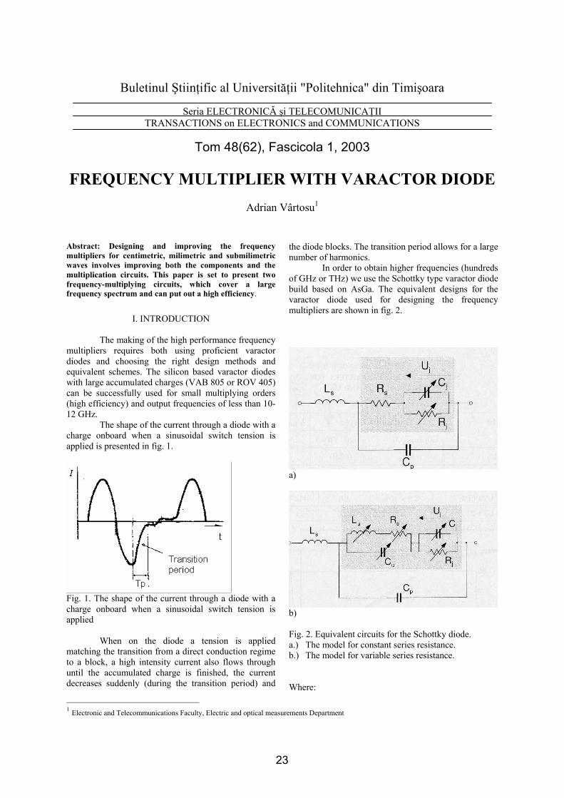
Abstract: Designing and improving the frequency multipliers for centimetric, milimetric and submilimetric waves involves improving both the components and the multiplication circuits. This paper is set to present two frequency-multiplying circuits, which cover a large frequency spectrum and can put out a high efficiency.

I. INTRODUCTION

The making of the high performance frequency

multipliers requires both using proficient varactor diodes and choosing the right design methods and equivalent schemes. The silicon based varactor diodes with large accumulated charges (VAB 805 or ROV 405) can be successfully used for small multiplying orders (high efficiency) and output frequencies of less than 10-12 GHz.

The shape of the current through a diode with a charge onboard when a sinusoidal switch tension is applied is presented in fig. 1.

Fig. 1. The shape of the current through a diode with a charge onboard when a sinusoidal switch tension is applied

When on the diode a tension is applied matching the transition from a direct conduction regime to a block, a high intensity current also flows through until the accumulated charge is finished, the current decreases suddenly (during the transition period) and

the diode blocks. The transition period allows for a large number of harmonics.

In order to obtain higher frequencies (hundreds of GHz or THz) we use the Schottky type varactor diode build based on AsGa. The equivalent designs for the varactor diode used for designing the frequency multipliers are shown in fig. 2.

a)

b)

Fig. 2. Equivalent circuits for the Schottky diode. a.) The model for constant series resistance. b.) The model for variable series resistance. Where:

23

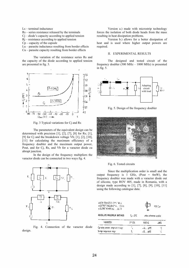
Ls – terminal inductance Rs – series resistance released by the terminals Cj – diode’s capacity according to applied tension Rj – resistance according to applied tension Cp – capacity of the capsule Lu – parasite inductance resulting from border effects Cu – parasite capacity resulting from border effects

The variation of the resistance series Rs and the capacity of the diode according to applied tension are presented in fig. 3.

Fig. 3 Typical variations for Cj and Rs The parameters of the equivalent design can be

determined with precision [1], [2], [7], [8] for Rs; [1], [9] for Cj and the breakdown voltage Vb; [1], [2], [10], [11] for calculating the maximum efficiency of a frequency doubler and the maximum output power, Pout, and for Cj, Rs, and Vb for a varactor diode cu abrupt junction.

In the design of the frequency multipliers the varactor diode can be connected in two ways fig. 4.

Fig. 4. Connection of the varactor diode

design.

Version a.) made with microstrip technology forces the isolation of both diode heads from the mass resulting in heat dissipation problems.

Version b.) allows for a better dissipation of heat and is used where higher output powers are required.

II. EXPERIMENTAL RESULTS The designed and tested circuit of the

frequency doubler (500 MHz – 1000 MHz) is presented in fig. 5.

Fig. 5. Design of the frequency doubler

Fig. 6. Tested circuits Since the multiplication order is small and the

output frequency is 1 GHz, (Pout = 4mW), the frequency doubler was made with a varactor diode out of silicone, type ROV 405, made in Romania, with a design made according to [1], [7], [8], [9], [10], [11] using the following catalogue data:

Adapting circuit

with load

24

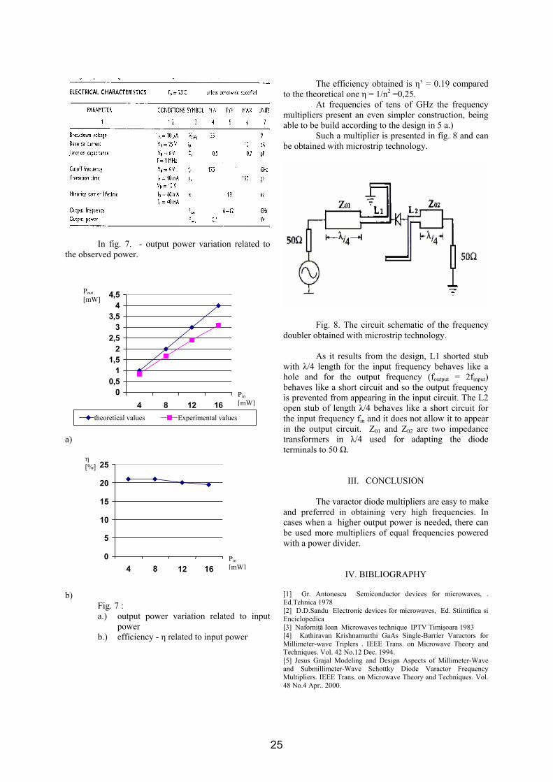
In fig. 7. - output power variation related to

the observed power. a) b)

Fig. 7 : a.) output power variation related to input

power b.) efficiency - η related to input power

The efficiency obtained is η’ = 0.19 compared to the theoretical one η = 1/n2 =0,25.

At frequencies of tens of GHz the frequency multipliers present an even simpler construction, being able to be build according to the design in 5 a.)

Such a multiplier is presented in fig. 8 and can be obtained with microstrip technology.

Fig. 8. The circuit schematic of the frequency

doubler obtained with microstrip technology. As it results from the design, L1 shorted stub

with λ/4 length for the input frequency behaves like a hole and for the output frequency (foutput = 2finput) behaves like a short circuit and so the output frequency is prevented from appearing in the input circuit. The L2 open stub of length λ/4 behaves like a short circuit for the input frequency fin and it does not allow it to appear in the output circuit. Z01 and Z02 are two impedance transformers in λ/4 used for adapting the diode terminals to 50 Ω.

III. CONCLUSION

The varactor diode multipliers are easy to make and preferred in obtaining very high frequencies. In cases when a higher output power is needed, there can be used more multipliers of equal frequencies powered with a power divider.

IV. BIBLIOGRAPHY

[1] Gr. Antonescu Semiconductor devices for microwaves, . Ed.Tehnica 1978 [2] D.D.Sandu Electronic devices for microwaves, Ed. Stiintifica si Enciclopedica [3] Naforniţă Ioan Microwaves technique IPTV Timişoara 1983 [4] Kathiravan Krishnamurthi GaAs Single-Barrier Varactors for Millimeter-wave Triplers . IEEE Trans. on Microwave Theory and Techniques. Vol. 42 No.12 Dec. 1994. [5] Jesus Grajal Modeling and Design Aspects of Millimeter-Wave and Submillimeter-Wave Schottky Diode Varactor Frequency Multipliers. IEEE Trans. on Microwave Theory and Techniques. Vol. 48 No.4 Apr.. 2000.

Pout [mW]

Pin [mW]

00,5

11,5

22,5

33,5

44,5

4 8 12 16valori teoretice valori experimentale

η [%]

Pin [mW]

0

5

10

15

20

25

4 8 12 16

theoretical values Experimental values

25

[6] Thomas C. Ho A W-Band Integrated Power Module Using MMIC MESFET Power Amplifiers and Varactor Doublers. IEEE Trans. on Microwave Theory and Techniques. Vol. 41 No.12 Dec. 1993. [7] J.A.Calvielo “High performance quasi-planar varactors for millimeter waves.” IEEE Trans. Electron Devices, vol. ED-21 oct 1974 [8] J.A.Calvielo , “Advanced devices and components for the millimeter and sub-millimeter systems,” IEEE Trans. Electron Devices, vol. ED-26, sept 1979.

[9] S.M.Sze High Speed Semiconductor Device. New York: Wiley Interscience, 1990. [10] T.C.Leonard , “Prediction of power and efficiency of frequency doublers using varactors exhibitingg general nonlinearity, “ Proc. IEEE, aug. 1963. [11] P.Penfield, Varactor Application. Cambridge, MA: MIT Press, 1962.

26

Buletinul Ştiinţific al Universităţii "Politehnica" din Timişoara

Seria ELECTRONICĂ şi TELECOMUNICAŢII TRANSACTIONS on ELECTRONICS and COMMUNICATIONS

Tom 48(62), Fascicola 1, 2003

ADC Testing by Beat Frequency and Envelope Methods

Daniel Belega 1

1 Dept. of Measurements and Optical Electronics, Faculty of Electronics and Telecommunications, e-mail: belega@etc.utt.ro

Abstract - The beat frequency and envelope methods are qualitative test methods that REVEAL the dynamic failures of an analog-to-digital converter (ADC). Thus, these methods do not provide quantitative information about the dynamic performances of the ADC under test. In this paper the dynamic performances of a real high-speed ADC were examined in the case of testing by beat frequency and envelope methods. The results obtained permit an appreciation concerning the ADC quality. Keywords: beat frequency method, envelope method, parameter estimation, interpolated FFT algorithm.

I. INTRODUCTION An important issue in testing high-speed analog-to-digital converters (ADCs) is their response to high frequency analog inputs. The test signals are sinewaves because they are the easiest to generate in practice at the frequency of interest with adequate fidelity. The dynamic performances of a high-speed ADC decrease when the analog input frequency increases and may degrade drastically as the analog input frequency approaches fs/2, where fs is the ADC maximum sampling frequency. Thus, to appreciate the ADC quality it is very useful to know the ADC dynamic performances for analog input frequencies very close to fs/2. However, because the ADC dynamic performances tend to degrade as the analog input frequency increases it is also very useful to know the ADC dynamic performances for analog input frequency very close to fs (i.e. very close to the superior limit of the ADC bandwidth), even this situation is seldom found in practice. The test method in which the sinewave input frequency differs from fs by a small incremental frequency is known as beat frequency method. The test method in which the frequency of the sinewave input is equal to fs/2 plus a small incremental frequency is know as envelope method. The main drawback of these methods is that they are qualitative methods [1], which puts in evidence the dynamic failures of an ADC. So, these methods do not provide quantitative information about the dynamic performances of the ADC under test. In this paper the dynamic performances of a real high-speed ADC were determinate when the ADC is tested

by beat frequency and envelope methods. Were estimated ones of the most important ADC dynamic parameters: signal to noise and distortion ratio (SINAD) and the effective number of bits (ENOB). These parameters were estimated by the algorithm proposed in [2].

II. BEAT FREQUENCY AND ENVELOPE METHODS

The beat frequency method provides a quick, qualitative demonstration of the ADC dynamic performance [1]. The input frequency finb is equal with the ADC sampling frequency fs = 1/Ts plus a small increment ∆f, i.e.

.fff sinb ∆+= (1)

The ideal ADC output sinewave is

( )

1,,1,0

,2sin 0

−=

+⎟⎟⎠

⎞⎜⎜⎝

⎛ϕ+π=

Mm

dmfs

fAmy inb

b

K

(2)

where A is the amplitude of the sinewave, equal to half of the ADC’s full-scale range (FSR), A = FSR/2;

ϕ0 is the phase of the input sinewave; d is the offset of the input sinewave; M is the number of samples acquired. By substituting (1) in (2) we obtain

( )

.1,,1,0

,2sin

22sin

0

0

−=

+⎟⎟⎠

⎞⎜⎜⎝

⎛ϕ+

∆π

=+⎟⎟⎠

⎞⎜⎜⎝

⎛ϕ+

∆π+π=

Mm

dmfsf

A

dmfsf

mAmyb

K

(3)

From (3) it follows that the ideal ADC output sinewave is a sinewave of ∆f frequency or beat frequency. So, the visualization of the samples

27

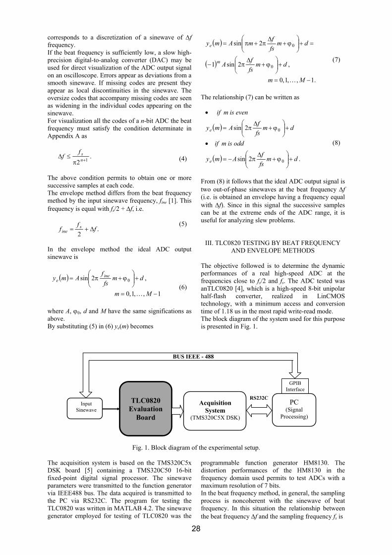
corresponds to a discretization of a sinewave of ∆f frequency. If the beat frequency is sufficiently low, a slow high-precision digital-to-analog converter (DAC) may be used for direct visualization of the ADC output signal on an oscilloscope. Errors appear as deviations from a smooth sinewave. If missing codes are present they appear as local discontinuities in the sinewave. The oversize codes that accompany missing codes are seen as widening in the individual codes appearing on the sinewave. For visualization all the codes of a n-bit ADC the beat frequency must satisfy the condition determinate in Appendix A as

.2 1+π

≤∆nsf

f

(4)

The above condition permits to obtain one or more successive samples at each code. The envelope method differs from the beat frequency method by the input sinewave frequency, fine [1]. This frequency is equal with fs/2 + ∆f, i.e.

.2

ff

f sine ∆+=

(5)

In the envelope method the ideal ADC output sinewave is

( )

1,,1,0

,2sin 0

−=

+⎟⎟⎠

⎞⎜⎜⎝

⎛ϕ+π=

Mm

dmfs

fAmy ine

e

K

(6)

where A, ϕ0, d and M have the same significations as above. By substituting (5) in (6) ye(m) becomes

( )

( )

.1,,1,0

,2sin1

2sin

0

0

−=

+⎟⎟⎠

⎞⎜⎜⎝

⎛ϕ+

∆π−

=+⎟⎟⎠

⎞⎜⎜⎝

⎛ϕ+

∆π+π=

Mm

dmfsf

A

dmfsf

mAmy

m

e

K

(7)

The relationship (7) can be written as

( )

( ) .2sin

2sin

0

0

dmfsfAmy

oddismif

dmfsf

Amy

evenismif

e

e

+⎟⎟⎠

⎞⎜⎜⎝

⎛ϕ+

∆π−=

•

+⎟⎟⎠

⎞⎜⎜⎝

⎛ϕ+

∆π=

•

(8)

From (8) it follows that the ideal ADC output signal is two out-of-phase sinewaves at the beat frequency ∆f (i.e. is obtained an envelope having a frequency equal with ∆f). Since in this signal the successive samples can be at the extreme ends of the ADC range, it is useful for analyzing slew problems.

III. TLC0820 TESTING BY BEAT FREQUENCY AND ENVELOPE METHODS

The objective followed is to determine the dynamic performances of a real high-speed ADC at the frequencies close to fs/2 and fs. The ADC tested was anTLC0820 [4], which is a high-speed 8-bit unipolar half-flash converter, realized in LinCMOS technology, with a minimum access and conversion time of 1.18 us in the most rapid write-read mode. The block diagram of the system used for this purpose is presented in Fig. 1.

Fig. 1. Block diagram of the experimental setup.

The acquisition system is based on the TMS320C5x DSK board [5] containing a TMS320C50 16-bit fixed-point digital signal processor. The sinewave parameters were transmitted to the function generator via IEEE488 bus. The data acquired is transmitted to the PC via RS232C. The program for testing the TLC0820 was written in MATLAB 4.2. The sinewave generator employed for testing of TLC0820 was the

programmable function generator HM8130. The distortion performances of the HM8130 in the frequency domain used permits to test ADCs with a maximum resolution of 7 bits. In the beat frequency method, in general, the sampling process is noncoherent with the sinewave of beat frequency. In this situation the relationship between the beat frequency ∆f and the sampling frequency fs is

Input Sinewave

TLC0820 Evaluation

Board

Acquisition System

(TMS320C5X DSK)

RS232C PC

(Signal Processing)

GPIB Interface

BUS IEEE - 488

28

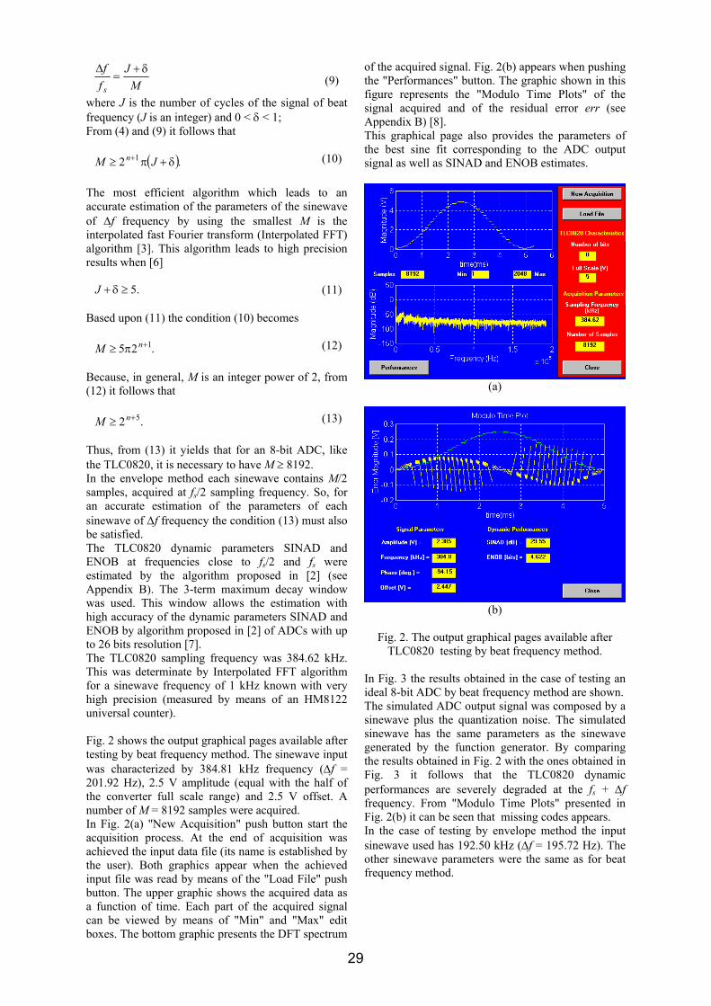
MJ

ff

s

δ+=

∆

(9)

where J is the number of cycles of the signal of beat frequency (J is an integer) and 0 < δ < 1; From (4) and (9) it follows that

( ).2 1 δ+π≥ + JM n (10)

The most efficient algorithm which leads to an accurate estimation of the parameters of the sinewave of ∆f frequency by using the smallest M is the interpolated fast Fourier transform (Interpolated FFT) algorithm [3]. This algorithm leads to high precision results when [6]

.5≥δ+J (11) Based upon (11) the condition (10) becomes

.25 1+π≥ nM (12) Because, in general, M is an integer power of 2, from (12) it follows that

.2 5+≥ nM (13) Thus, from (13) it yields that for an 8-bit ADC, like the TLC0820, it is necessary to have M ≥ 8192. In the envelope method each sinewave contains M/2 samples, acquired at fs/2 sampling frequency. So, for an accurate estimation of the parameters of each sinewave of ∆f frequency the condition (13) must also be satisfied. The TLC0820 dynamic parameters SINAD and ENOB at frequencies close to fs/2 and fs were estimated by the algorithm proposed in [2] (see Appendix B). The 3-term maximum decay window was used. This window allows the estimation with high accuracy of the dynamic parameters SINAD and ENOB by algorithm proposed in [2] of ADCs with up to 26 bits resolution [7]. The TLC0820 sampling frequency was 384.62 kHz. This was determinate by Interpolated FFT algorithm for a sinewave frequency of 1 kHz known with very high precision (measured by means of an HM8122 universal counter). Fig. 2 shows the output graphical pages available after testing by beat frequency method. The sinewave input was characterized by 384.81 kHz frequency (∆f = 201.92 Hz), 2.5 V amplitude (equal with the half of the converter full scale range) and 2.5 V offset. A number of M = 8192 samples were acquired. In Fig. 2(a) "New Acquisition" push button start the acquisition process. At the end of acquisition was achieved the input data file (its name is established by the user). Both graphics appear when the achieved input file was read by means of the "Load File" push button. The upper graphic shows the acquired data as a function of time. Each part of the acquired signal can be viewed by means of "Min" and "Max" edit boxes. The bottom graphic presents the DFT spectrum

of the acquired signal. Fig. 2(b) appears when pushing the "Performances" button. The graphic shown in this figure represents the "Modulo Time Plots" of the signal acquired and of the residual error err (see Appendix B) [8]. This graphical page also provides the parameters of the best sine fit corresponding to the ADC output signal as well as SINAD and ENOB estimates.

(a)

(b)

Fig. 2. The output graphical pages available after

TLC0820 testing by beat frequency method. In Fig. 3 the results obtained in the case of testing an ideal 8-bit ADC by beat frequency method are shown. The simulated ADC output signal was composed by a sinewave plus the quantization noise. The simulated sinewave has the same parameters as the sinewave generated by the function generator. By comparing the results obtained in Fig. 2 with the ones obtained in Fig. 3 it follows that the TLC0820 dynamic performances are severely degraded at the fs + ∆f frequency. From "Modulo Time Plots" presented in Fig. 2(b) it can be seen that missing codes appears. In the case of testing by envelope method the input sinewave used has 192.50 kHz (∆f = 195.72 Hz). The other sinewave parameters were the same as for beat frequency method.

29

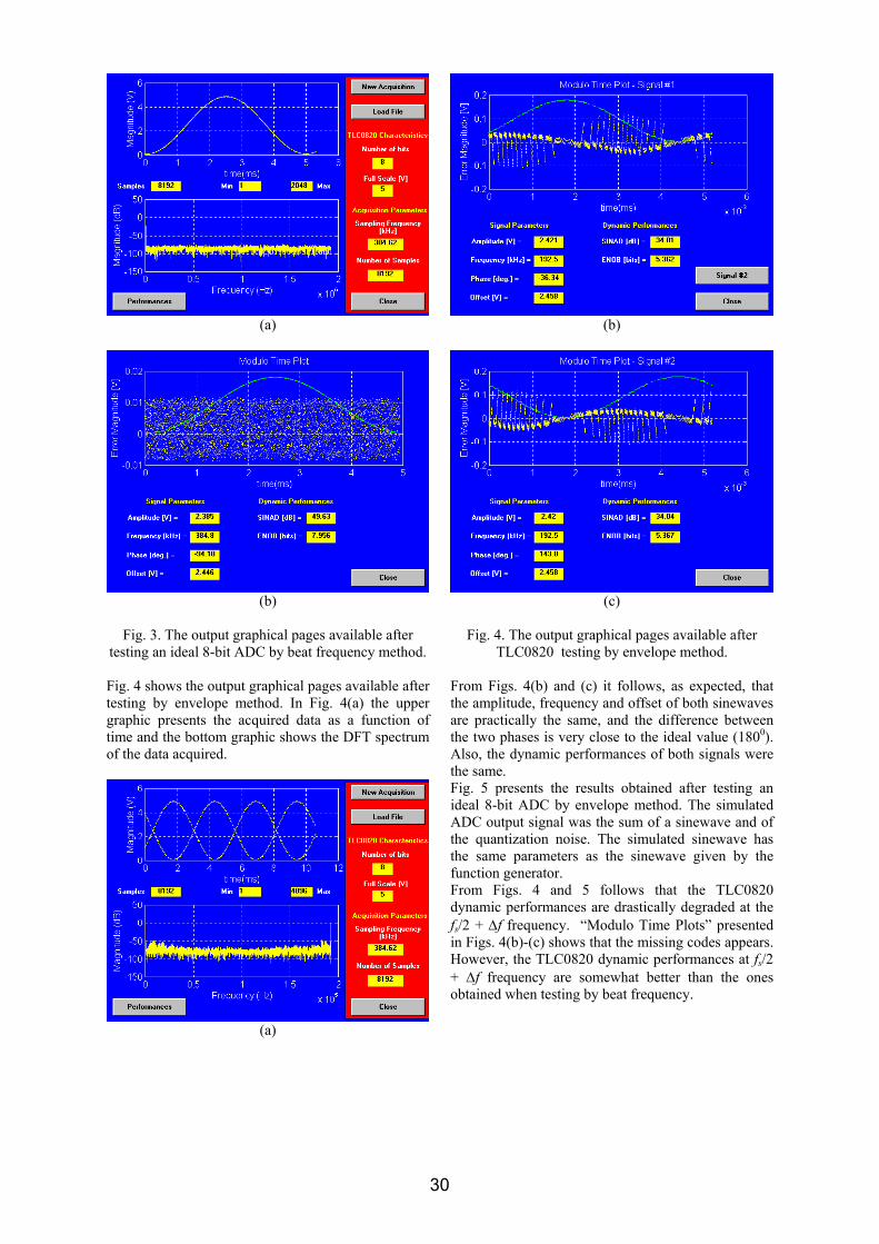
(a)

(b)

Fig. 3. The output graphical pages available after

testing an ideal 8-bit ADC by beat frequency method. Fig. 4 shows the output graphical pages available after testing by envelope method. In Fig. 4(a) the upper graphic presents the acquired data as a function of time and the bottom graphic shows the DFT spectrum of the data acquired.

(a)

(b)

(c)

Fig. 4. The output graphical pages available after

TLC0820 testing by envelope method.

From Figs. 4(b) and (c) it follows, as expected, that the amplitude, frequency and offset of both sinewaves are practically the same, and the difference between the two phases is very close to the ideal value (1800). Also, the dynamic performances of both signals were the same. Fig. 5 presents the results obtained after testing an ideal 8-bit ADC by envelope method. The simulated ADC output signal was the sum of a sinewave and of the quantization noise. The simulated sinewave has the same parameters as the sinewave given by the function generator. From Figs. 4 and 5 follows that the TLC0820 dynamic performances are drastically degraded at the fs/2 + ∆f frequency. “Modulo Time Plots” presented in Figs. 4(b)-(c) shows that the missing codes appears. However, the TLC0820 dynamic performances at fs/2 + ∆f frequency are somewhat better than the ones obtained when testing by beat frequency.

30

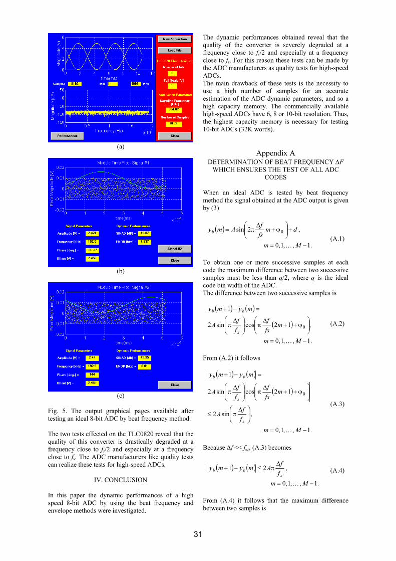
(a)

(b)

(c)

Fig. 5. The output graphical pages available after testing an ideal 8-bit ADC by beat frequency method. The two tests effected on the TLC0820 reveal that the quality of this converter is drastically degraded at a frequency close to fs/2 and especially at a frequency close to fs. The ADC manufacturers like quality tests can realize these tests for high-speed ADCs.

IV. CONCLUSION In this paper the dynamic performances of a high speed 8-bit ADC by using the beat frequency and envelope methods were investigated.

The dynamic performances obtained reveal that the quality of the converter is severely degraded at a frequency close to fs/2 and especially at a frequency close to fs. For this reason these tests can be made by the ADC manufacturers as quality tests for high-speed ADCs. The main drawback of these tests is the necessity to use a high number of samples for an accurate estimation of the ADC dynamic parameters, and so a high capacity memory. The commercially available high-speed ADCs have 6, 8 or 10-bit resolution. Thus, the highest capacity memory is necessary for testing 10-bit ADCs (32K words).

Appendix A DETERMINATION OF BEAT FREQUENCY ∆F

WHICH ENSURES THE TEST OF ALL ADC CODES

When an ideal ADC is tested by beat frequency method the signal obtained at the ADC output is given by (3)

( )

.1,,1,0

,2sin 0

−=

+⎟⎟⎠

⎞⎜⎜⎝

⎛ϕ+

∆π=

Mm

dmfsfAmyb

K

(A.1)

To obtain one or more successive samples at each code the maximum difference between two successive samples must be less than q/2, where q is the ideal code bin width of the ADC. The difference between two successive samples is

( ) ( )

( )

.1,,1,0

,12cossin2

1

0

−=

⎟⎟⎠

⎞⎜⎜⎝

⎛ϕ++

∆π⎟⎟

⎠

⎞⎜⎜⎝

⎛ ∆π

=−+

Mm

mfsf

ff

A

mymy

s

bb

K

(A.2)

From (A.2) it follows

( ) ( )

( )

.1,,1,0

,sin2

12cossin2

1

0

−=

⎟⎟⎠

⎞⎜⎜⎝

⎛ ∆π≤

⎟⎟⎠

⎞⎜⎜⎝

⎛ϕ++

∆π⎟⎟

⎠

⎞⎜⎜⎝

⎛ ∆π

=−+

MmffA

mfsf

ffA

mymy

s

s

bb

K

(A.3)

Because ∆f << fess (A.3) becomes

( ) ( )

.1,,1,0

,21

−=

∆π≤−+

MmffAmymys

bb

K

(A.4)

From (A.4) it follows that the maximum difference between two samples is

31

( ) ( )

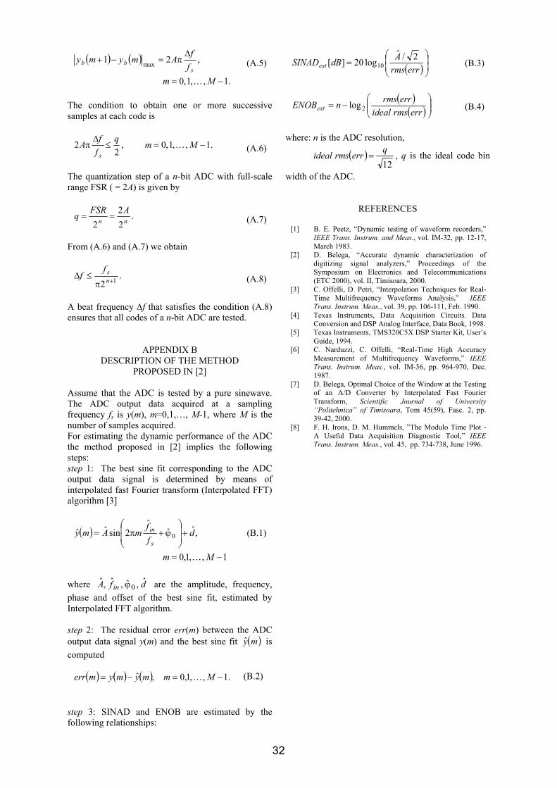
.1,,1,0

,21 max

−=

∆π=−+

MmffAmymys

bb

K

(A.5)

The condition to obtain one or more successive samples at each code is

.1,,1,0,2

2 −=≤∆

π MmqffAs

K (A.6)

The quantization step of a n-bit ADC with full-scale range FSR ( = 2A) is given by

.22

2 nnAFSRq ==

(A.7)

From (A.6) and (A.7) we obtain

.2 1+π

≤∆nsf

f (A.8)

A beat frequency ∆f that satisfies the condition (A.8) ensures that all codes of a n-bit ADC are tested.

APPENDIX B DESCRIPTION OF THE METHOD

PROPOSED IN [2] Assume that the ADC is tested by a pure sinewave. The ADC output data acquired at a sampling frequency fs is y(m), m=0,1,…, M-1, where M is the number of samples acquired. For estimating the dynamic performance of the ADC the method proposed in [2] implies the following steps: step 1: The best sine fit corresponding to the ADC output data signal is determined by means of interpolated fast Fourier transform (Interpolated FFT) algorithm [3]

( )

1,,1,0

,ˆˆˆ

2sinˆˆ 0

−=

+⎟⎟⎠

⎞⎜⎜⎝

⎛ϕ+π=

Mm

dff

mAmys

in

K

(B.1)

where dfA in

ˆ,ˆ,ˆ,ˆ0ϕ are the amplitude, frequency,

phase and offset of the best sine fit, estimated by Interpolated FFT algorithm. step 2: The residual error err(m) between the ADC output data signal y(m) and the best sine fit ( )my is computed

( ) ( ) ( ) .1,,1,0,ˆ −=−= Mmmymymerr K

(B.2)

step 3: SINAD and ENOB are estimated by the following relationships:

( )⎟⎟⎠

⎞⎜⎜⎝

⎛=

errrmsAdBSINADest

2/ˆlog20][ 10

(B.3)

( )

( )⎟⎟⎠

⎞⎜⎜⎝

⎛−=

errrmsidealerrrmsnENOBest 2log

(B.4)

where: n is the ADC resolution,

( )12qerrrmsideal = , q is the ideal code bin

width of the ADC.

REFERENCES

[1] B. E. Peetz, “Dynamic testing of waveform recorders,” IEEE Trans. Instrum. and Meas., vol. IM-32, pp. 12-17, March 1983.

[2] D. Belega, “Accurate dynamic characterization of digitizing signal analyzers,” Proceedings of the Symposium on Electronics and Telecommunications (ETC 2000), vol. II, Timisoara, 2000.

[3] C. Offelli, D. Petri, “Interpolation Techniques for Real-Time Multifrequency Waveforms Analysis,” IEEE Trans. Instrum. Meas., vol. 39, pp. 106-111, Feb. 1990.

[4] Texas Instruments, Data Acquisition Circuits. Data Conversion and DSP Analog Interface, Data Book, 1998.

[5] Texas Instruments, TMS320C5X DSP Starter Kit, User’s Guide, 1994.

[6] C. Narduzzi, C. Offelli, “Real-Time High Accuracy Measurement of Multifrequency Waveforms,” IEEE Trans. Instrum. Meas., vol. IM-36, pp. 964-970, Dec. 1987.

[7] D. Belega, Optimal Choice of the Window at the Testing of an A/D Converter by Interpolated Fast Fourier Transform, Scientific Journal of University “Politehnica” of Timisoara, Tom 45(59), Fasc. 2, pp. 39-42, 2000.

[8] F. H. Irons, D. M. Hummels, ”The Modulo Time Plot - A Useful Data Acquisition Diagnostic Tool,” IEEE Trans. Instrum. Meas., vol. 45, pp. 734-738, June 1996.

32

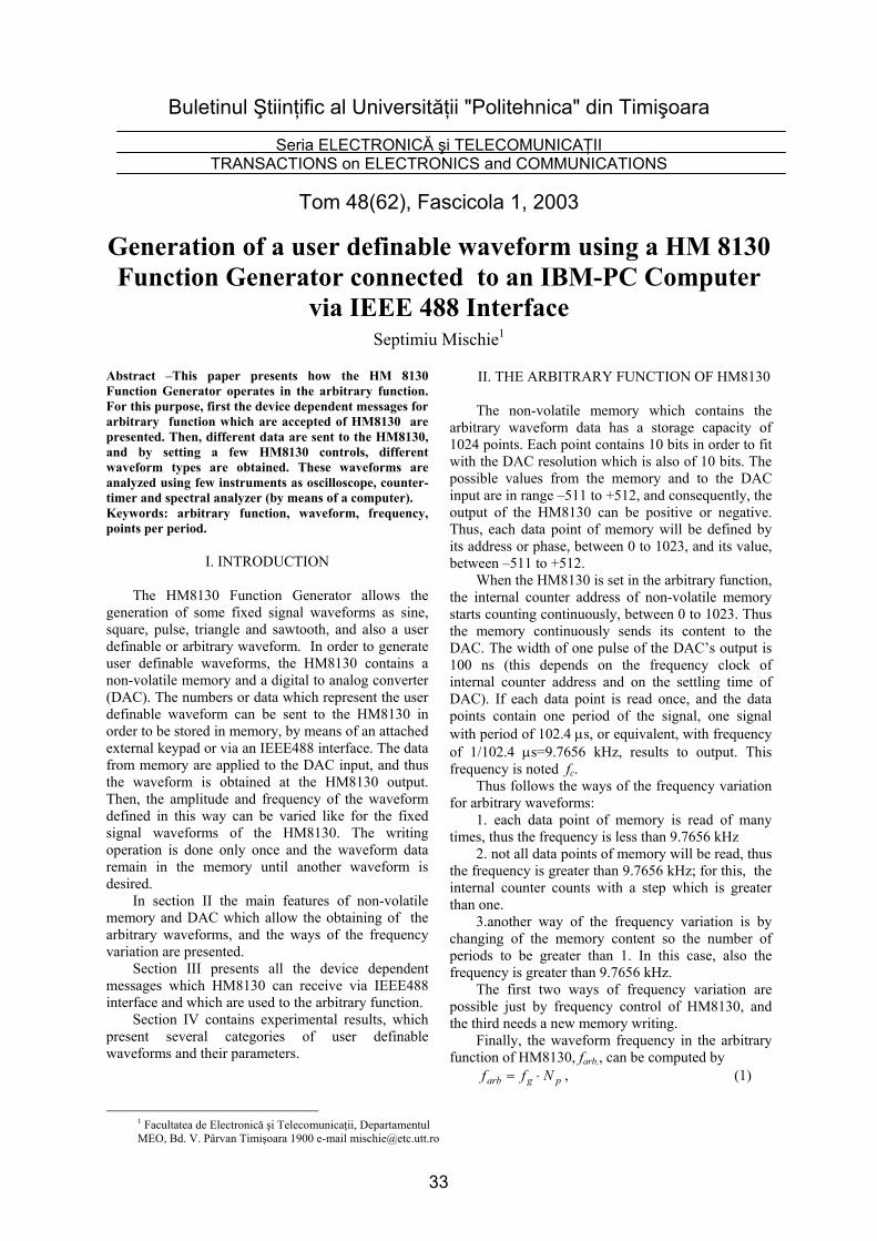
Buletinul Ştiinţific al Universităţii "Politehnica" din Timişoara

Seria ELECTRONICĂ şi TELECOMUNICAŢII TRANSACTIONS on ELECTRONICS and COMMUNICATIONS

Tom 48(62), Fascicola 1, 2003

Generation of a user definable waveform using a HM 8130 Function Generator connected to an IBM-PC Computer

via IEEE 488 Interface

Septimiu Mischie1

1 Facultatea de Electronică şi Telecomunicaţii, Departamentul MEO, Bd. V. Pârvan Timişoara 1900 e-mail mischie@etc.utt.ro

Abstract –This paper presents how the HM 8130 Function Generator operates in the arbitrary function. For this purpose, first the device dependent messages for arbitrary function which are accepted of HM8130 are presented. Then, different data are sent to the HM8130, and by setting a few HM8130 controls, different waveform types are obtained. These waveforms are analyzed using few instruments as oscilloscope, counter-timer and spectral analyzer (by means of a computer). Keywords: arbitrary function, waveform, frequency, points per period.

I. INTRODUCTION

The HM8130 Function Generator allows the generation of some fixed signal waveforms as sine, square, pulse, triangle and sawtooth, and also a user definable or arbitrary waveform. In order to generate user definable waveforms, the HM8130 contains a non-volatile memory and a digital to analog converter (DAC). The numbers or data which represent the user definable waveform can be sent to the HM8130 in order to be stored in memory, by means of an attached external keypad or via an IEEE488 interface. The data from memory are applied to the DAC input, and thus the waveform is obtained at the HM8130 output. Then, the amplitude and frequency of the waveform defined in this way can be varied like for the fixed signal waveforms of the HM8130. The writing operation is done only once and the waveform data remain in the memory until another waveform is desired.

In section II the main features of non-volatile memory and DAC which allow the obtaining of the arbitrary waveforms, and the ways of the frequency variation are presented.

Section III presents all the device dependent messages which HM8130 can receive via IEEE488 interface and which are used to the arbitrary function.

Section IV contains experimental results, which present several categories of user definable waveforms and their parameters.

II. THE ARBITRARY FUNCTION OF HM8130 The non-volatile memory which contains the

arbitrary waveform data has a storage capacity of 1024 points. Each point contains 10 bits in order to fit with the DAC resolution which is also of 10 bits. The possible values from the memory and to the DAC input are in range –511 to +512, and consequently, the output of the HM8130 can be positive or negative. Thus, each data point of memory will be defined by its address or phase, between 0 to 1023, and its value, between –511 to +512.

When the HM8130 is set in the arbitrary function, the internal counter address of non-volatile memory starts counting continuously, between 0 to 1023. Thus the memory continuously sends its content to the DAC. The width of one pulse of the DAC’s output is 100 ns (this depends on the frequency clock of internal counter address and on the settling time of DAC). If each data point is read once, and the data points contain one period of the signal, one signal with period of 102.4 µs, or equivalent, with frequency of 1/102.4 µs=9.7656 kHz, results to output. This frequency is noted fc.

Thus follows the ways of the frequency variation for arbitrary waveforms:

1. each data point of memory is read of many times, thus the frequency is less than 9.7656 kHz

2. not all data points of memory will be read, thus the frequency is greater than 9.7656 kHz; for this, the internal counter counts with a step which is greater than one.

3.another way of the frequency variation is by changing of the memory content so the number of periods to be greater than 1. In this case, also the frequency is greater than 9.7656 kHz.

The first two ways of frequency variation are possible just by frequency control of HM8130, and the third needs a new memory writing.

Finally, the waveform frequency in the arbitrary function of HM8130, farb,, can be computed by

pgarb Nff ⋅= , (1)

33

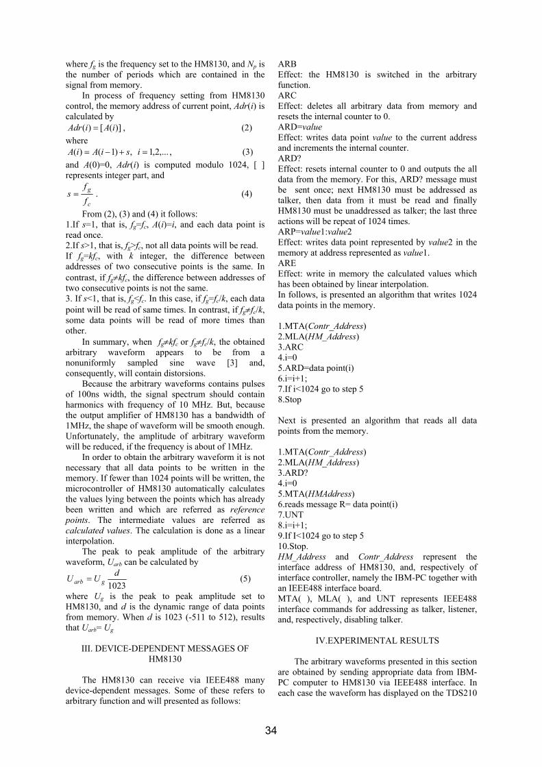
where fg is the frequency set to the HM8130, and Np is the number of periods which are contained in the signal from memory. In process of frequency setting from HM8130 control, the memory address of current point, Adr(i) is calculated by

)]([)( iAiAdr = , (2) where

,...2,1,)1()( =+−= isiAiA , (3) and A(0)=0, Adr(i) is computed modulo 1024, [ ] represents integer part, and

c

g

ff

s = . (4)

From (2), (3) and (4) it follows: 1.If s=1, that is, fg=fc, A(i)=i, and each data point is read once. 2.If s>1, that is, fg>fc, not all data points will be read. If fg=kfc, with k integer, the difference between addresses of two consecutive points is the same. In contrast, if fg≠kfc, the difference between addresses of two consecutive points is not the same. 3. If s<1, that is, fg<fc. In this case, if fg=fc/k, each data point will be read of same times. In contrast, if fg≠fc/k, some data points will be read of more times than other. In summary, when fg≠kfc or fg≠fc/k, the obtained arbitrary waveform appears to be from a nonuniformly sampled sine wave [3] and, consequently, will contain distorsions. Because the arbitrary waveforms contains pulses of 100ns width, the signal spectrum should contain harmonics with frequency of 10 MHz. But, because the output amplifier of HM8130 has a bandwidth of 1MHz, the shape of waveform will be smooth enough. Unfortunately, the amplitude of arbitrary waveform will be reduced, if the frequency is about of 1MHz. In order to obtain the arbitrary waveform it is not necessary that all data points to be written in the memory. If fewer than 1024 points will be written, the microcontroller of HM8130 automatically calculates the values lying between the points which has already been written and which are referred as reference points. The intermediate values are referred as calculated values. The calculation is done as a linear interpolation. The peak to peak amplitude of the arbitrary waveform, Uarb can be calculated by

1023dUU garb = (5)

where Ug is the peak to peak amplitude set to HM8130, and d is the dynamic range of data points from memory. When d is 1023 (-511 to 512), results that Uarb= Ug

III. DEVICE-DEPENDENT MESSAGES OF

HM8130 The HM8130 can receive via IEEE488 many device-dependent messages. Some of these refers to arbitrary function and will presented as follows:

ARB Effect: the HM8130 is switched in the arbitrary function. ARC Effect: deletes all arbitrary data from memory and resets the internal counter to 0. ARD=value Effect: writes data point value to the current address and increments the internal counter. ARD? Effect: resets internal counter to 0 and outputs the all data from the memory. For this, ARD? message must be sent once; next HM8130 must be addressed as talker, then data from it must be read and finally HM8130 must be unaddressed as talker; the last three actions will be repeat of 1024 times. ARP=value1:value2 Effect: writes data point represented by value2 in the memory at address represented as value1. ARE Effect: write in memory the calculated values which has been obtained by linear interpolation. In follows, is presented an algorithm that writes 1024 data points in the memory. 1.MTA(Contr_Address) 2.MLA(HM_Address) 3.ARC 4.i=0 5.ARD=data point(i) 6.i=i+1; 7.If i<1024 go to step 5 8.Stop Next is presented an algorithm that reads all data points from the memory. 1.MTA(Contr_Address) 2.MLA(HM_Address) 3.ARD? 4.i=0 5.MTA(HMAddress) 6.reads message R= data point(i) 7.UNT 8.i=i+1; 9.If I<1024 go to step 5 10.Stop. HM_Address and Contr_Address represent the interface address of HM8130, and, respectively of interface controller, namely the IBM-PC together with an IEEE488 interface board. MTA( ), MLA( ), and UNT represents IEEE488 interface commands for addressing as talker, listener, and, respectively, disabling talker.

IV.EXPERIMENTAL RESULTS The arbitrary waveforms presented in this section are obtained by sending appropriate data from IBM-PC computer to HM8130 via IEEE488 interface. In each case the waveform has displayed on the TDS210

34

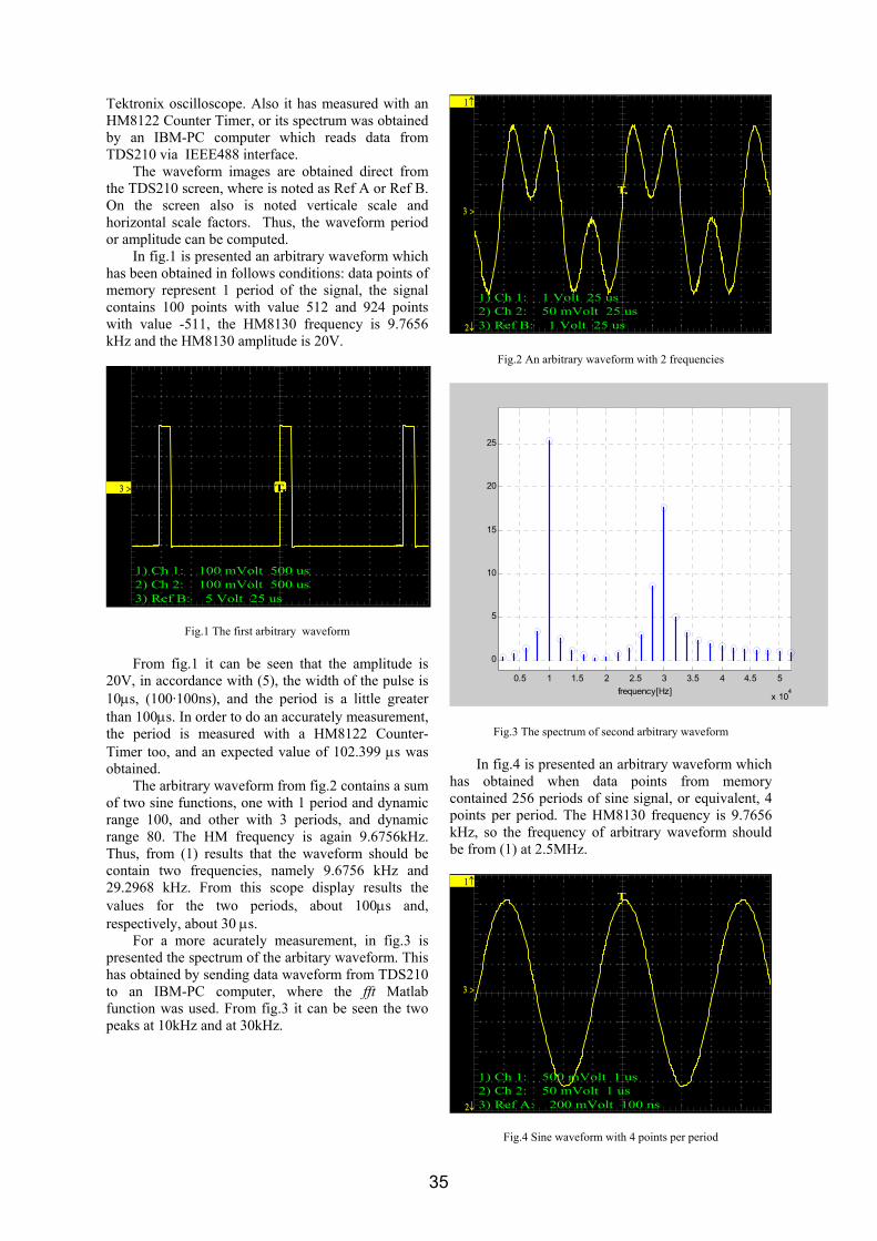
Tektronix oscilloscope. Also it has measured with an HM8122 Counter Timer, or its spectrum was obtained by an IBM-PC computer which reads data from TDS210 via IEEE488 interface.

The waveform images are obtained direct from the TDS210 screen, where is noted as Ref A or Ref B. On the screen also is noted verticale scale and horizontal scale factors. Thus, the waveform period or amplitude can be computed.

In fig.1 is presented an arbitrary waveform which has been obtained in follows conditions: data points of memory represent 1 period of the signal, the signal contains 100 points with value 512 and 924 points with value -511, the HM8130 frequency is 9.7656 kHz and the HM8130 amplitude is 20V.

TT1 >2 >3 >

1) Ch 1: 100 mVolt 500 us 2) Ch 2: 100 mVolt 500 us 3) Ref B: 5 Volt 25 us

Fig.1 The first arbitrary waveform

From fig.1 it can be seen that the amplitude is 20V, in accordance with (5), the width of the pulse is 10µs, (100·100ns), and the period is a little greater than 100µs. In order to do an accurately measurement, the period is measured with a HM8122 Counter-Timer too, and an expected value of 102.399 µs was obtained.

The arbitrary waveform from fig.2 contains a sum of two sine functions, one with 1 period and dynamic range 100, and other with 3 periods, and dynamic range 80. The HM frequency is again 9.6756kHz. Thus, from (1) results that the waveform should be contain two frequencies, namely 9.6756 kHz and 29.2968 kHz. From this scope display results the values for the two periods, about 100µs and, respectively, about 30 µs.

For a more acurately measurement, in fig.3 is presented the spectrum of the arbitary waveform. This has obtained by sending data waveform from TDS210 to an IBM-PC computer, where the fft Matlab function was used. From fig.3 it can be seen the two peaks at 10kHz and at 30kHz.

TT

1↑

2↓

3 >

1) Ch 1: 1 Volt 25 us 2) Ch 2: 50 mVolt 25 us 3) Ref B: 1 Volt 25 us

Fig.2 An arbitrary waveform with 2 frequencies

0.5 1 1.5 2 2.5 3 3.5 4 4.5 5

x 104

0

5

10

15

20

25

frequency[Hz]

Fig.3 The spectrum of second arbitrary waveform

In fig.4 is presented an arbitrary waveform which has obtained when data points from memory contained 256 periods of sine signal, or equivalent, 4 points per period. The HM8130 frequency is 9.7656 kHz, so the frequency of arbitrary waveform should be from (1) at 2.5MHz.

T1↑

2↓

3 >

1) Ch 1: 500 mVolt 1 us 2) Ch 2: 50 mVolt 1 us 3) Ref A: 200 mVolt 100 ns

Fig.4 Sine waveform with 4 points per period

35

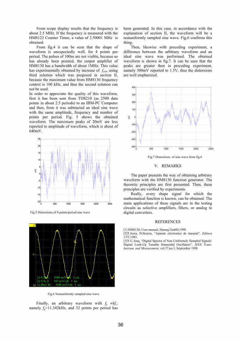
From scope display results that the frequency is about 2.5 MHz. If the frequency is measured with the HM8122 Counter Timer, a value of 2.50001 MHz is obtained. From fig.4 it can be seen that the shape of waveform is unexpectedly well, for 4 points per period. The pulses of 100ns are not visible, because so has already been pointed, the output amplifier of HM8130 has a bandwidth of about 1MHz. This value has experimentally obtained by increase of farb, using third solution which was proposed in section II, because the maximum value from HM8130 frequency control is 100 kHz, and thus the second solution can not be used. In order to appreciate the quality of this waveform, first it has been sent from TDS210 (as 2500 data points in about 2.5 periods) to an IBM-PC Computer and then, from it was subtracted an ideal sine wave with the same amplitude, frequency and number of points per period. Fig. 5 shows the obtained waveform. The maximum peaks of 20mV are less reported to amplitude of waveform, which is about of 640mV.

0 500 1000 1500 2000 2500-20

-15

-10

-5

0

5

10

15

20

25

mV

Fig.5 Distorsions of 4 points/period sine wave

TT

1↑

2↓

3 >

1) Ch 1: 500 mVolt 1 us 2) Ch 2: 50 mVolt 1 us 3) Ref B: 500 mVolt 1 us

Fig.6 Nonuniformly sampled sine wave

Finally, an arbitrary waveform with fg ≠kfc, namely fg=11.342kHz, and 32 points per period has

been generated. In this case, in accordance with the explanation of section II, the waveform will be a nonuniformly sampled sine wave. Fig.6 confirms this thing. Then, likewise with preceding experiment, a difference between the arbitrary waveform and an ideal sine wave was performed. The obtained waveform is shown in fig.7. It can be seen that the peaks are greater then in preceding experiment, namely 300mV reported to 1.5V, thus the distorsions are well emphasized.

0 500 1000 1500 2000 2500-400

-300

-200

-100

0

100

200

300

400

mV

Fig.7 Distorsions of sine wave from fig.6

V. REMARKS The paper presents the way of obtaining arbitrary waveform with the HM8130 function generator. The theoretic principles are first presented. Then, these principles are verified by experiments. Really, every shape signal for which the mathematical function is known, can be obtained. The main applications of these signals are in the testing circuits as selective amplifiers, filters, or analog to digital converters.

REFERENCES [1] HM8130, User manual, Hameg GmbH,1998 [2]T.Jurca, D.Stoiciu, “Aparate electronice de masurat”, Editura UTT,1993. [3]Y.C.Jenq, “Digital Spectra of Non-Uniformely Sampled Signals-Digital Look-Up Tunable Sinusoidal Oscillators”, IEEE Trans. Instrum. and Measurement, vol.37,no.3, September 1998

36

Buletinul Ştiinţific al Universităţii "Politehnica" din Timişoara

Seria ELECTRONICĂ şi TELECOMUNICAŢII TRANSACTIONS on ELECTRONICS and COMMUNICATIONS

Tom 48(62), Fascicola 1, 2003

Some Aspects Regarding Frequency Analysis of the Nonlinear Systems

Georgeta Budura1

1 Facultatea de Electronică şi Telecomunicaţii, Departamentul Comunicaţii Bd. V. Pârvan Timişoara 1900 e-mail getab@ee.utt.ro

Abstract – The Volterra model for nonlinear systems has develloped an identity of its one. We concentrate in this paper of some aspects regarding the characterization of the Volterra system in the frequency domain. Both types of filters are considered: analogues and discretized filters. The applications of the second order kernel transform are widely investigated in bouth cases. Finnaly we derive and analyze the input-output power transfer relationship. Two situations are considered: in the first one the input signal has Gaussian statistics, in the second one there is a little knowledge about the input statistics or the input is non-Gaussian. It is also noted that the ordinary coherence functions cannot be used in explaining the input-output power transfer relationship of a quadratic system excitated by a non-gaussian input signal. Keywords: Frequency domain Volterra filters, Second order kernel transform, input-output power transfer relationship.

I. INTRODUCTION

The Volterra series has been applied widely as nonlinear system modeling technique with considerable success. A difficulty encountered when one wants to apply the Volterra functional series to nonlinear problems involves the measurement of the Volterra kernels. Thus one of the major tasks in Volterra modeling is to determine the Volterra kernels(in time domain) or the Volterra transfer functions (in the frequency domain). Frequency domain methods for identification Volterra kernels have been widely explore . In this paper we presented theoretical results to handle Volterra filters in the frequency domain. In the theory of Volterra operators,

][iH , the transform of the different orders kernels also play an important role in analysis and synthesis. Also looking at the Fourier transform of the output of a Volterra filter gives a profound insight in the physical interpretation of those nonlinear filters. We begin our study, in Section II, with a derivation of the second order kernel transform which is then interpreted through various applications. To do this we first develop the two-dimensional Fourier

transform. Our development is obtained from the one-dimensional theory of Fourier transform. We consider first analogues Volterra filters and then the discreet Volterra filters. In Section III we derive and analyze the input-output power transfer relationship. Two situations are considered: in the first one the input signal has Gaussian statistics, in the second one there is a little knowledge about the input statistics or the input is non-Gaussian. It is also noted that the ordinary coherence functions cannot be used in explaining the input-output power transfer relationship of a quadratic system excitated by a non-gaussian input signal. It is often possible to satisfy the Gaussian assumption when the input excitation is under control of the experimentalist. In many practical cases, however, the input excitation is not under the direct control of the experimentalist.

II. THE VOLTERRA MODEL IN THE FREQUENCY DOMAIN

2.1 Volterra Filtering On Continuous Signals

Consider a nonlinear, continuous, finite-memory, time-invariant, single-input, single-output, causal system. According to the theorem by Frechet, such a system can be uniformly approximated, over a uniformly bounded equicontinuous set of inputs, to an arbitrary degree of accuracy by a Volterra series of sufficient but finite order [1]. If the system is single-input single-output and the finite order is I then the series takes the form:

( ) ( ) ( ) iiii

I

iiddtxtxhty ττττττ LLLL 111

0 0)( −−= ∫∑∫

=

∞

(1) Here x(t) is the system input and hi are the Volterra kernels, essentially multidimensional weighting functions in the Volterra series. In practice the upper limits of the integrals are set equal to T, the duration of the finite memory of the system.

37

The input-output relation (1) can be rewrite using the nonlinear operators of different orders:

)]([)]([)]([)( 210 txHtxHtxHHty n++++= K (2) For example the second order Volterra operator is defined by [1]:

∫ ∫∞

∞−

∞

∞−

−−= 21212122 )()(),()]([ ττττττ dtxtxhtxH (3)

In the theory of nonlinear Volterra operators the transform of the n-order kernel plays an important role in analysis and synthesis. We begin our discussion with a derivation of the second order kernel transform. The function H2(ω1, ω2) called the transform of the second order Volterra kernel is defined by [1]:

∫ ∫∞

∞−

∞

∞−

+−= 21)(

2122122211),(),( ττττωω τωτω ddehH j (4)

The condition sufficient to ensure the existence of the Fourier transform of the kernel h2 is:

⟨∞∫ ∫∞

∞−

∞

∞−21212 ),( ττττ dh (5)

The inverse relation is:

∫ ∫∞

∞−

∞

∞−

+= 21)(

21222122211),(

)2(1),( ωωωωπ

ττ τωτω deHh j

(6) As a first application of the second-order kernel transform, we consider the response of the operator

][2H for the sinusoidal input, tAtx 0cos)( ω= :

),(Re2

2

),(Re2

2)(

002

2

2002

20

ωω

ωω ω

−⎟⎠⎞

⎜⎝⎛

+⎟⎠⎞

⎜⎝⎛=

HA

eHAty tj

(7)

The response is seen to contain a costant (given by the second term in (7)) and a sinusoid of frequency 2ω0

and amplitude ),(2 0022

ωω −⎟⎠⎞⎜

⎝⎛ HA .

If the surface of the absolute value of the second-order kernel transform ),( 212 ωωH is plotted as a function of ω1 and ω2., then the output constant is proportional to the height of the surface along a

045− line in the 21 ωω − plane. We thus observe that the sinusoidal response of the second-order operator H2 does not characterize the system, since the response is determined only by the values of the kernel transform along the lines 21 ωω = and

21 ωω −= . This is different than the result for a stable first-order operator which is completely characterized by the sinusoidal response. Another application where the second-order kernel transform can be used is to express the input- output relation in the frequency domain when the input is a transient function [2]. Let )(2 ty be the response of a second order Volterra filter to a transient input signal )(tx , given by (3). The Fourier transform of a transient response and a transient input are, respectively,

∫∞

∞−

−= dtetyY tjωω )()( (8)

and

∫∞

∞−

−= dtetxX tjωω )()( (9)

We desired to express )(ωY in terms of )(ωX and

).,( 212 ωωH We first defined the artificial function ),( 21)2( tty according to (10):

∫ ∫∞

∞−

∞

∞−

−−= 21221121221)2( )()(),(),( ττττττ dtxtxhtty

(10)

We can observe that )(),()2( tytty =

The Two-dimensional Fourier transform of ),( 212 tty is:

∫ ∫∞

∞−

∞

∞−

+−= 21)(

21)2(21)2(2211),(),( dtdtettyY ttj ωωωω (11)

We now substitute eq.(8) in eq.(11) and obtain:

)()(),(),( 2121221)2( ωωωωωω XXHY = (12) In the eq.(12) ),( 212 ωωH is the kernel transform of

),( 212 ττh and )(ωX is the Fourier transform of the input x(t) . According to the inverse transform we have:

∫ ∫∞

∞−

∞

∞−

+== 21)(

21)2(2)2(2211),(

)2(1)()( ωωωωπ

ωω ddeYtyty ttj

(13)

The desired form is obtained by making the substitution: 21 ωωω += .

∫ ∫∞

∞−

∞

∞−

−= 111)2(2 ),()2(

1)( ωωωωωπ

ω ddeYty tj (14)

Analyzing eq.(14) we observe that y(t) is the inverse transform of the function:

38

111)2( ),(21)( ωωωωπ

ω ∫∞

∞−

−= dYY (15)

2.2 Volterra Filtering On Discretized Signals

In practical application, in the case of identification of real systems, the input and output signals are digitalized, and the identification technique is performed numerically on computers. The prototype for Volterra filtering on discretized signals is the second order Volterra filter (SVF). We will consider next a rigorous presentation in the frequency domain of the SVF. The input-output relationship in the case of SVF is:

][][],[

][][][

2

1

0

1

01212

1

01110

1 2

1

knxknxkkh

knxkhhny

N

k

N

k

N

k

−−

+−+=

∑ ∑

∑−

=

−

=

−

= (16)

where ][ 11 kh and ],[ 212 kkh are called the linear and quadratic filter weights, respectively, and N denotes the filter length. The quadratic filter weights are assumed to be symmetric, i.e., ],[],[ 122212 kkhkkh = . The Fourier transform of the second order kernel is:

∑ ∑−

=

−

=

Ω−Ω−=ΩΩ1

0

1

0212212

1 2

2211],[),(N

k

N

k

kjkj eekkhH (17)

The transform of the second order kernel has many applications. We consider next the frequency response of the SVF to a transient input. We will consider only the contribution of the second order kernel, ][2 ny , defined by the third term in rel. (16). As in continuous case we define the artificial function:

∑ ∑−

=

−

=

−−=1

0

1

0221121221)2(

1 2

][][],[],[N

k

N

kknxknxkkhnny

(18)The bidimensional Fourier of ],[ 21)2( nny is given by:

∑ ∑ ∑ ∑∞

=

∞

=

−

=

−

=

Ω−Ω−−−

=ΩΩ

0 0

1

0

1

02211212

21)2(

1 2 1 2

2211][][],[

),(

n n

N

k

N

k

njnj eeknxknxkkh

Y

(19) By making the change of variables 111 knu −= and

222 knu −= we can separate the quadruple sum into the product of sums that can be express in terms of ),( 212 ΩΩH and )(ΩX :

)()(),(),( 2121221)2( ΩΩΩΩ=ΩΩ XXHY (20)

),( 21)2( ΩΩY is called the bispectral response of the

second order kernel to the input signal )(ΩX . Considering that ],[][ )2(2 nnyny = we can express

][2 ny , as the inverse transform of:

∫ ΩΩ−ΩΩ=Ωππ 2

111)2(2 ),(21)( dYY (21)

The operation defined by (21) transforms a function on the ),( 21 ΩΩ plane to another function of Ω by integrating the first along the line 21 Ω+Ω=Ω . Considering also the contribution of the first order kernel the response of the SVF is:

∫ ΩΩ−ΩΩ+ΩΩ=Ωππ 2

111)2(112 ),(21)()()( dYXHY

(22) In the following we apply the eq. (22) to derive the response of the SVF to a Gaussian, ergodig input signal of zero mean and finite statistical moments up to fourth order. The autocorrelation function of the input is:

][][12

1lim][ 2121 knxknxN

kkrN

Nnnxx −−+

=− ∑−=∞→

(23)

Requiring the unbiasness of the filter output we have:

∑ ∑−

=

−

=

−−=1

0

1

0212120

1 2

][],[N

k

N

kxx kkrkkhh (24)

By combining (16) and (24) the output of the SVF output is expressed as:

∑ ∑

∑−

=

−

=

−

=

−−−−

+−+=

1

0

1

02121212

1

01110

1 2

1

][][][],[

][][][

N

k

N

kxx

N

k

kkrknxknxkkh

knxkhhny

(25)

The autocorrelation function of the output is:

∑−=∞→

++

=N

NnNyy nyknyN

kr ][][12

1lim][ (26)

According to the properties of Gaussian variables [3] express by (27)

434232

4131214321

321 0

xxxxxx

xxxxxxxxxx

xxx

++

+++=

=

(27)

we have:

39

][][],[],[2

][][][][

2121212212

1

0,,,

212111

1

0,

2121

21

kllrkkkrllhkkh

kkkrkhkhkr

xxxx

N

llkk

xx

N

kkyy

+−+−

−+−=

−

=

−

=

∑∑

∑∑

(28)

We also define the power spectral densities of ][nx and ][ny as:

∑

∑∞

−∞=

Ω−

∞

−∞=

Ω−

=ΩΦ

=ΩΦ

k

kjyyyy

k

kjxxxx

ekr

ekr

][)(

][)( (29)

Then, from the duality between the multidimensional convolution and the Fourier transform, it can be shown that:

∫ ΩΩ−ΩΩΦ+ΩΦΩ=ΩΦπ

π2

111)2(2

11 ),(212)(()( dH yyxxyy

(30) where:

)()(,(),( 212

21221)2( ΩΦΩΦΩΩ=ΩΩΦ xxxxyy H (31) The cross-spectral power density between

][ny and ][nx is [4]:

∑∞

−∞=

Ω−=ΩΦk

jkyxxy ekr ][)( (32)

where:

∑−=∞→

+=N

Nnnyx knxnyN

kr ][][21lim][ (33)

Finally we get:

)()()( 1 ΩΦΩ=ΩΦ xxxy H (34) which is a familiar result from linear system theory and is due to the property given by eq.(27). We can also define the cross-bispectral density between ][ny and ][nx as [4]:

)(21

,21

2211

21

],[),( Ω+Ω−∞

−∞=∑∑=ΩΩ kkj

xykk

xy ekktS (35)

where:

][][][12

1lim],[ 2121 knxknxnyN

kktN

Nnnyx +++

= ∑−=∞→

(36) represents the cross-bicorrelation function between

][ny and ][nx . The equation (35) can be rewritten as:

)()(),(2),( 2121221 ΩΦΩΦΩΩ=ΩΩ xxxxxy HS (37) Note from the above equation that the cross-bispectral density can specify the function ),( 212 ΩΩH

uniquely, assuming that )( ΩΦ xx is known and 0)( ≠ΩΦ xx for all Ф. This also reveals the possibility that one can compute the Quadratic transfer function directly from (37), using an estimate of the cross-bispectral density. This technique, called cross-bispectral analysis, can be implemented efficiently by using the FFT algorithm.

III. INPUT-OUTPUT POWER RELATIONSHIP Since we will concentrate on the frequency domain analysis the system model to be studied will be expressed follows [5]:

)()(),()()()( 2)1(,

1 jiji

M

mjiMji

mmm fXfXffHfXfHfY

=+−−=

∑∑+=

(38)

where )( mfX and )( mfY respectively represent the discret Fourier transforms(DFT’s) for a finite number (N) of observations of the input and output signals of the system described by a Volterra series up to second order, and 2/NM ff = signifies the Nyquist frequency associated with the sampling of the time domain signals. On the other hand, )(1 mfH and

),(2 ji ffH are the linear and quadratic transfer functions given at a discret set of frequencies:

2/,,2,1,0,1,2,,12/,/ NNnNnfn LL −−+−== . One can express the linear and quadratic transfer functions in terms of the input and output characteristics by solving the following set of equations which are obtained by multiplying (38) by

)(*mfX and )()( **

ji fXfX respectively, and then taking an expected value of each side. To simplify notation fm will be denoted as m, etc.

)]()()([

),(])([)()]()([

*

2,

21

*

jXiXmXE

jiHmXEmHmYmXE

mjiji

⋅

+=

=+

∑∑

(39)

)]()()()([),(

)]()()([)()]()()([**

2,

**1

**

jXiXlXkXEjiH

mXlXkXEmHmYlXkXE

mjiji=+

∑∑+=

(40) In (39) and (40) , ][⋅E denotes the expectation operator . Note that the right-hand side of (40)

40

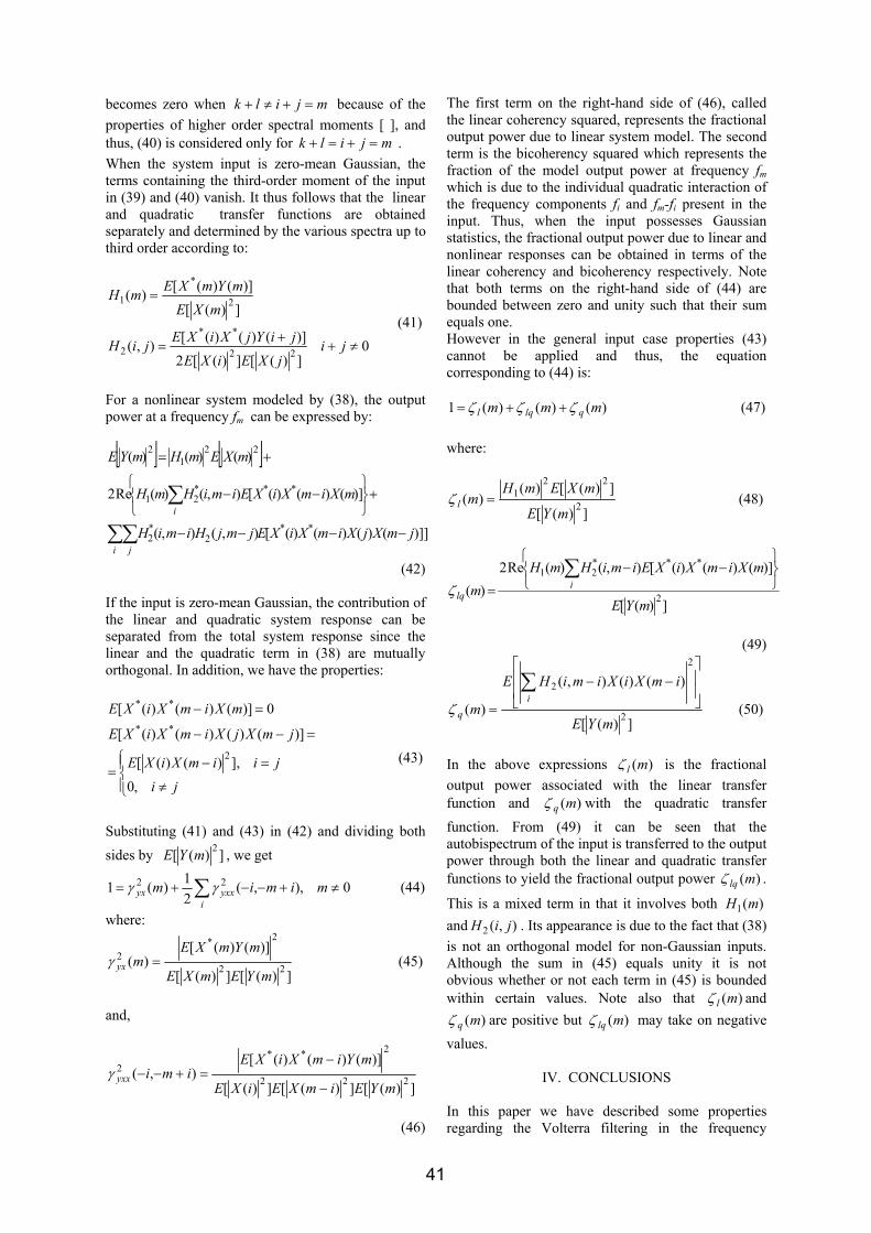
becomes zero when mjilk =+≠+ because of the properties of higher order spectral moments [ ], and thus, (40) is considered only for mjilk =+=+ . When the system input is zero-mean Gaussian, the terms containing the third-order moment of the input in (39) and (40) vanish. It thus follows that the linear and quadratic transfer functions are obtained separately and determined by the various spectra up to third order according to:

0])([])([2)]()()([),(

])([)]()([)(

22

**

2

2

*

1

≠++

=

=

jijXEiXE

jiYjXiXEjiH

mXEmYmXEmH

(41)

For a nonlinear system modeled by (38), the output power at a frequency fm can be expressed by: [ ] [ ]

)]]()()()([),(),(

)]()()([),()(Re2

)()()(

**2

*2

***21

221

2

jmXjXimXiXEjmjHimiH

mXimXiXEimiHmH

mXEmHmYE

i j

i

−−−−

+⎭⎬⎫

⎩⎨⎧

−−

+=

∑∑

∑

(42)

If the input is zero-mean Gaussian, the contribution of the linear and quadratic system response can be separated from the total system response since the linear and the quadratic term in (38) are mutually orthogonal. In addition, we have the properties:

⎪⎩

⎪⎨⎧

≠

=−=

=−−

=−

jijiimXiXE

jmXjXimXiXE

mXimXiXE

,0],)()([

)]()()()([

0)]()()([

2

**

**

(43)

Substituting (41) and (43) in (42) and dividing both sides by ])([ 2mYE , we get

∑ ≠+−−+=i

yxxyx mimim 0),,(21)(1 22 γγ (44)

where:

])([])([

)]()([)( 22

2*2

mYEmXE

mYmXEmyx =γ (45)

and,

])([])([])([

)]()()([),( 222

2**2

mYEimXEiXE

mYimXiXEimiyxx

−

−=+−−γ

(46)

The first term on the right-hand side of (46), called the linear coherency squared, represents the fractional output power due to linear system model. The second term is the bicoherency squared which represents the fraction of the model output power at frequency fm which is due to the individual quadratic interaction of the frequency components fi and fm-fi present in the input. Thus, when the input possesses Gaussian statistics, the fractional output power due to linear and nonlinear responses can be obtained in terms of the linear coherency and bicoherency respectively. Note that both terms on the right-hand side of (44) are bounded between zero and unity such that their sum equals one. However in the general input case properties (43) cannot be applied and thus, the equation corresponding to (44) is:

)()()(1 mmm qlql ζζζ ++= (47) where:

])([

])([)()( 2

221

mYE

mXEmHml =ζ (48)

])([

)]()()([),()(Re2)( 2

***21

mYE

mXimXiXEimiHmHm i

lq⎭⎬⎫

⎩⎨⎧

−−

=∑

ζ

(49)

])([

)()(),(

)( 2

2

2

mYE

imXiXimiHE

mi

q

⎥⎥

⎦

⎤

⎢⎢

⎣

⎡−−

=

∑ζ (50)

In the above expressions )(mlζ is the fractional output power associated with the linear transfer function and )(mqζ with the quadratic transfer function. From (49) it can be seen that the autobispectrum of the input is transferred to the output power through both the linear and quadratic transfer functions to yield the fractional output power )(mlqζ .

This is a mixed term in that it involves both )(1 mH and ),(2 jiH . Its appearance is due to the fact that (38) is not an orthogonal model for non-Gaussian inputs. Although the sum in (45) equals unity it is not obvious whether or not each term in (45) is bounded within certain values. Note also that )(mlζ and

)(mqζ are positive but )(mlqζ may take on negative values.

IV. CONCLUSIONS

In this paper we have described some properties regarding the Volterra filtering in the frequency

41

domain. We considered both case: continuous signals and discretized signals. We applied the theoretical results to derive the Volterra filter response to different signals. Un important case is represented by the evaluation of the filter response to an input signal which is Gaussian and has zero mean. The input-output relation in the frequency domain reveals important properties of the second order Volterra filter. Finally we evaluated the input-output power relationship. In the theory of nonlinear Volterra operators the transform of the n-order kernel plays an important role in analysis and synthesis. This relation permit to evaluate the contribution of each order operator on the Output power of the Volterra filter: the contribution due to the linear operator is represented by the linear coherency squared, while the contribution due to the quadratic operator is represented by the bicoherency squared function. This case corespond to an input signal which is Gaussian. For a general random input, of unknown statistics, we have demonstrated that the autobispectrum of the input is transferred to the output power through both the linear and quadratic transfer functions to yield the fractional output power )(mlqζ .

This is a mixed term in that it involves both )(1 mH and ),(2 jiH .

REFERENCES

[1] Schetzen, M., The Volterra and Wiener theories of nonlinear systems”, Wiley and Sons, New York, 1980. [2] Budura, G., “Contributii privind studiul sistemelor neliniare utilizând seriile Volterra”, Teză de doctorat, UPT, Timişoara, 1999. [3] Morthensen R.E., “Random Signals and Systems”, John Wiley & Sons, 1987. [4] Koh, T., Powers, E., J., “Second Order Volterra Filtering and its Application to Nonlinear System Identification” IEEE Trans on ASSP, Vol. ASSP-33, No. 6, pag.1445-1455, decembrie 1985. [5] Kim, K., I., Powers, E., J., “A Digital Method of Modeling Quadratic Nonlinear Systems with a General Random Input”, IEEE Trans on ASSP, vol.36, No. 11, pag. 1758-1769, Noiembrie 1988.

42

Buletinul Ştiinţific al Universităţii "Politehnica" din Timişoara

Seria ELECTRONICĂ şi TELECOMUNICAŢII TRANSACTIONS on ELECTRONICS and COMMUNICATIONS

Tom 48(62), Fascicola 1, 2003

Analysis and Modeling of Systems withNonlinearities

Georgeta Budura, Corina Botoca1

1 Facultatea de Electronică şi Telecomunicaţii, Departamentul Comunicaţii Bd. V. Pârvan Timişoara 1900 e-mail getab@ee.utt.ro

Abstract – Without going into great mathematical detail, this paper discusses the polynomial models of nonlinearity. At first we have mentioned the important applications in telecommunications area that made the model very popular. In all the applications considered nonlinear models are used to characterize and compensate the effects of unwanted nonlinearities. Such systems should ideally be linear; therefore nonlinearities constitute an imperfection in the systems. Two types of systems are considered: nonlinear systems without memory and nonlinear systems with memory. In both cases we try to represent low order nonlinearities. For representing memoryless nonlinearities we considered the power series and the sets of orthogonal polynomials. Nonlinear systems with memory are modeled by the Volterra series and the orthogonal Wiener functionals. Original contributions have been made regarding the performance of models considered. Keywords: Systems with nonlinearities in telecommunications, Power series representation, Volterra and Wiener models.

I. INTRODUCTION Linear systems are useful in a large number of applications. Analysis, modeling and implementation of such filters are relatively straightforward tasks in many applications. However there are several situations in which the performance of linear filters is unacceptable. A simple but omnipresent type of nonlinearity is the saturation –type nonlinearity. Trying to identify these types of systems using linear models can often give misleading results. Another situation where nonlinear models will do well when linear models will have unacceptable performance is that of trying to relate two signals with no overlapping spectral components. When confronted with nonlinear systems problems many researchers shy away from the situation mainly because the solutions are often difficult from an analytical and/or computational point of view. Moreover, the rich variety of highly developed tools available for solving linear systems engineering problems are just not there when it comes to most nonlinear systems problems. Without going into great mathematical detail, this paper will discuss

two common models of nonlinearity. Also, a tutorial style has been adopted throughout. 1.1 Motivation: The Necessity Of Nonlinear Models

To Improve System Performances Specific applications (for illustration) that need nonlinear structures are encountered in many area. The dynamic development of nonlinear filtering is indicated by the amount of research presently published and the popularity and wide spread use of nonlinear digital filters in a variety of applications, notably in telecommunications, image processing, in geophysical and biomedical signal processing. System analysis using nonlinear structures has many applications. High-speed communications channels often need nonlinear equalizers for acceptable performance. Although channel equalization using linear tap delay line structures is adequate in many applications, there are several other situations when they will not work at all. For example, error probability performance of data transmission systems operating at rates better than 4800 bits/s due almost entirely to nonlinear distortion [1]. In telephone transmission, nonlinearities arise principally from inaccuracies in signal compounding. In digital satellite links, the satellite amplifiers are usually driven to near the saturation point and they exhibit highly nonlinear characteristics. Several researchers have used nonlinear models [2], [3], [4], [5], [6], to implement nonlinear channel equalizers [7], [8], [9], [10], [11], [12], [13]. Acoustic echo cancellers (AECs) in today’s hands-free telephones and video conferencing systems rely on the assumption of linear echo path. However, low cost audio equipment or constraints of portable communication systems cause nonlinear distortions in the loud speaker and its amplifier which limit the echo reduction of linear AECs. This means that an annoying nonlinearly distorted echo (“nonlinear echo”) will be transmitted back to the far end subscriber especially at loud speech portions [14], [15], [16], [17], [18].

43

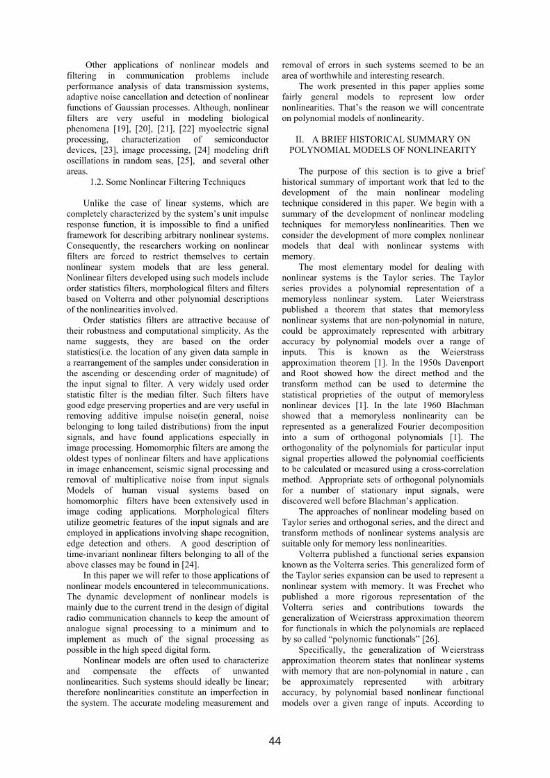
Other applications of nonlinear models and filtering in communication problems include performance analysis of data transmission systems, adaptive noise cancellation and detection of nonlinear functions of Gaussian processes. Although, nonlinear filters are very useful in modeling biological phenomena [19], [20], [21], [22] myoelectric signal processing, characterization of semiconductor devices, [23], image processing, [24] modeling drift oscillations in random seas, [25], and several other areas.

1.2. Some Nonlinear Filtering Techniques

Unlike the case of linear systems, which are completely characterized by the system’s unit impulse response function, it is impossible to find a unified framework for describing arbitrary nonlinear systems. Consequently, the researchers working on nonlinear filters are forced to restrict themselves to certain nonlinear system models that are less general. Nonlinear filters developed using such models include order statistics filters, morphological filters and filters based on Volterra and other polynomial descriptions of the nonlinearities involved. Order statistics filters are attractive because of their robustness and computational simplicity. As the name suggests, they are based on the order statistics(i.e. the location of any given data sample in a rearrangement of the samples under consideration in the ascending or descending order of magnitude) of the input signal to filter. A very widely used order statistic filter is the median filter. Such filters have good edge preserving properties and are very useful in removing additive impulse noise(in general, noise belonging to long tailed distributions) from the input signals, and have found applications especially in image processing. Homomorphic filters are among the oldest types of nonlinear filters and have applications in image enhancement, seismic signal processing and removal of multiplicative noise from input signals Models of human visual systems based on homomorphic filters have been extensively used in image coding applications. Morphological filters utilize geometric features of the input signals and are employed in applications involving shape recognition, edge detection and others. A good description of time-invariant nonlinear filters belonging to all of the above classes may be found in [24]. In this paper we will refer to those applications of nonlinear models encountered in telecommunications. The dynamic development of nonlinear models is mainly due to the current trend in the design of digital radio communication channels to keep the amount of analogue signal processing to a minimum and to implement as much of the signal processing as possible in the high speed digital form. Nonlinear models are often used to characterize and compensate the effects of unwanted nonlinearities. Such systems should ideally be linear; therefore nonlinearities constitute an imperfection in the system. The accurate modeling measurement and

removal of errors in such systems seemed to be an area of worthwhile and interesting research. The work presented in this paper applies some fairly general models to represent low order nonlinearities. That’s the reason we will concentrate on polynomial models of nonlinearity.

II. A BRIEF HISTORICAL SUMMARY ON POLYNOMIAL MODELS OF NONLINEARITY

The purpose of this section is to give a brief historical summary of important work that led to the development of the main nonlinear modeling technique considered in this paper. We begin with a summary of the development of nonlinear modeling techniques for memoryless nonlinearities. Then we consider the development of more complex nonlinear models that deal with nonlinear systems with memory. The most elementary model for dealing with nonlinear systems is the Taylor series. The Taylor series provides a polynomial representation of a memoryless nonlinear system. Later Weierstrass published a theorem that states that memoryless nonlinear systems that are non-polynomial in nature, could be approximately represented with arbitrary accuracy by polynomial models over a range of inputs. This is known as the Weierstrass approximation theorem [1]. In the 1950s Davenport and Root showed how the direct method and the transform method can be used to determine the statistical proprieties of the output of memoryless nonlinear devices [1]. In the late 1960 Blachman showed that a memoryless nonlinearity can be represented as a generalized Fourier decomposition into a sum of orthogonal polynomials [1]. The orthogonality of the polynomials for particular input signal properties allowed the polynomial coefficients to be calculated or measured using a cross-correlation method. Appropriate sets of orthogonal polynomials for a number of stationary input signals, were discovered well before Blachman’s application. The approaches of nonlinear modeling based on Taylor series and orthogonal series, and the direct and transform methods of nonlinear systems analysis are suitable only for memory less nonlinearities. Volterra published a functional series expansion known as the Volterra series. This generalized form of the Taylor series expansion can be used to represent a nonlinear system with memory. It was Frechet who published a more rigorous representation of the Volterra series and contributions towards the generalization of Weierstrass approximation theorem for functionals in which the polynomials are replaced by so called “polynomic functionals” [26]. Specifically, the generalization of Weierstrass approximation theorem states that nonlinear systems with memory that are non-polynomial in nature , can be approximately represented with arbitrary accuracy, by polynomial based nonlinear functional models over a given range of inputs. According to

44

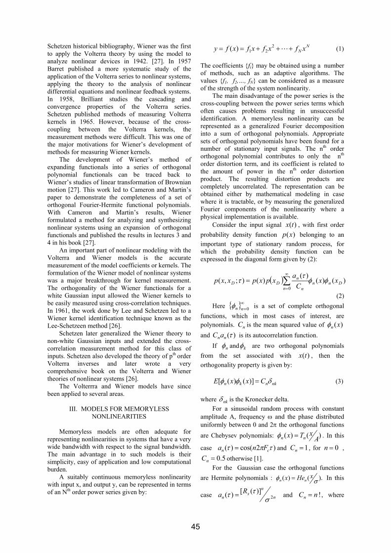
Schetzen historical bibliography, Wiener was the first to apply the Volterra theory by using the model to analyze nonlinear devices in 1942. [27]. In 1957 Barret published a more systematic study of the application of the Volterra series to nonlinear systems, applying the theory to the analysis of nonlinear differential equations and nonlinear feedback systems. In 1958, Brilliant studies the cascading and convergence properties of the Volterra series. Schetzen published methods of measuring Volterra kernels in 1965. However, because of the cross-coupling between the Volterra kernels, the measurement methods were difficult. This was one of the major motivations for Wiener’s development of methods for measuring Wiener kernels. The development of Wiener’s method of expanding functionals into a series of orthogonal polynomial functionals can be traced back to Wiener’s studies of linear transformation of Brownian motion [27]. This work led to Cameron and Martin’s paper to demonstrate the completeness of a set of orthogonal Fourier-Hermite functional polynomials. With Cameron and Martin’s results, Wiener formulated a method for analyzing and synthesizing nonlinear systems using an expansion of orthogonal functionals and published the results in lectures 3 and 4 in his book [27]. An important part of nonlinear modeling with the Volterra and Wiener models is the accurate measurement of the model coefficients or kernels. The formulation of the Wiener model of nonlinear systems was a major breakthrough for kernel measurement. The orthogonality of the Wiener functionals for a white Gaussian input allowed the Wiener kernels to be easily measured using cross-correlation techniques. In 1961, the work done by Lee and Schetzen led to a Wiener kernel identification technique known as the Lee-Schetzeen method [26]. Schetzen later generalized the Wiener theory to non-white Gaussian inputs and extended the cross-correlation measurement method for this class of inputs. Schetzen also developed the theory of pth order Volterra inverses and later wrote a very comprehensive book on the Volterra and Wiener theories of nonlinear systems [26]. The Volterrra and Wiener models have since been applied to several areas.

III. MODELS FOR MEMORYLESS NONLINEARITIES

Memoryless models are often adequate for representing nonlinearities in systems that have a very wide bandwidth with respect to the signal bandwidth. The main advantage in to such models is their simplicity, easy of application and low computational burden.

A suitably continuous memoryless nonlinearity with input x, and output y, can be represented in terms of an Nth order power series given by:

NN xfxfxfxfy +++== L2

21)( (1)

The coefficients fi may be obtained using a number of methods, such as an adaptive algorithms. The values f1, f2,…, fN can be considered as a measure of the strength of the system nonlinearity.

The main disadvantage of the power series is the cross-coupling between the power series terms which often causes problems resulting in unsuccessful identification. A memoryless nonlinearity can be represented as a generalized Fourier decomposition into a sum of orthogonal polynomials. Appropriate sets of orthogonal polynomials have been found for a number of stationary input signals. The nth order orthogonal polynomial contributes to only the nth order distortion term, and its coefficient is related to the amount of power in the nth order distortion product. The resulting distortion products are completely uncorrelated. The representation can be obtained either by mathematical modeling in case where it is tractable, or by measuring the generalized Fourier components of the nonlinearity where a physical implementation is available.

Consider the input signal )(tx , with first order probability density function )(xp belonging to an important type of stationary random process, for which the probability density function can be expressed in the diagonal form given by (2):

( ) )()()(

)();,(0

Dnnn n

nDD xx

Ca

xpxpxxp φφτ

τ ∑∞

=

=

(2) Here ∞=0nnφ is a set of complete orthogonal

functions, which in most cases of interest, are polynomials. nC is the mean squared value of )(xnφ and )(τnnaC is its autocorrelation function.

If nφ and kφ are two orthogonal polynomials from the set associated with )(tx , then the orthogonality property is given by:

nknkn CxxE δφφ =)]()([ (3)

where nkδ is the Kronecker delta.

For a sinusoidal random process with constant amplitude A, frequency ω and the phase distributed uniformly between 0 and 2π the orthogonal functions are Chebysev polynomials: )()( A

xTx nn =φ . In this

case )2cos()( τπτ cn Fna = and 1=nC , for 0=n , 5.0=nC otherwise [1].

For the Gaussian case the orthogonal functions are Hermite polynomials : ).()( σφ xHex nn = In this

case n

nx

nRa 2

)]([)(σ

ττ = and !nCn = , where

45

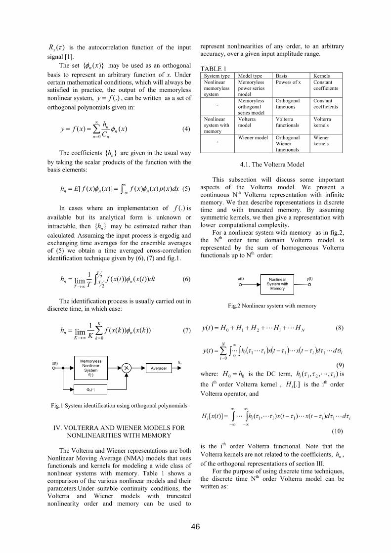
)(τxR is the autocorrelation function of the input signal [1].

The set )( xnφ may be used as an orthogonal basis to represent an arbitrary function of x. Under certain mathematical conditions, which will always be satisfied in practice, the output of the memoryless nonlinear system, (.)fy = , can be written as a set of orthogonal polynomials given in:

∑∞

=

==0

)()(n

nn

n xChxfy φ (4)

The coefficients nh are given in the usual way

by taking the scalar products of the function with the basis elements:

∫∞

∞−== dxxpxxfxxfEh nnn )()()()]()([ φφ (5)

In cases where an implementation of (.)f is

available but its analytical form is unknown or intractable, then nh may be estimated rather than calculated. Assuming the input process is ergodig and exchanging time averages for the ensemble averages of (5) we obtain a time averaged cross-correlation identification technique given by (6), (7) and fig.1.

∫−∞→

= 2

2))(())((1

limT

T nT

n dttxtxfT

h φ (6)

The identification process is usually carried out in

discrete time, in which case:

∑=∞→

=K

kn

Kn kxkxf

Kh

0))(())((1

lim φ (7)

Fig.1 System identification using orthogonal polynomials

IV. VOLTERRA AND WIENER MODELS FOR NONLINEARITIES WITH MEMORY

The Volterra and Wiener representations are both Nonlinear Moving Average (NMA) models that uses functionals and kernels for modeling a wide class of nonlinear systems with memory. Table 1 shows a comparison of the various nonlinear models and their parameters.Under suitable continuity conditions, the Volterra and Wiener models with truncated nonlinearity order and memory can be used to

represent nonlinearities of any order, to an arbitrary accuracy, over a given input amplitude range. TABLE 1

System type Model type Basis Kernels Nonlinear memoryless system

Memoryless power series model

Powers of x Constant coefficients

˝

Memoryless orthogonal series model

Orthogonal functions

Constant coefficients

Nonlinear system with memory

Volterra model

Volterra functionals

Volterra kernels

˝

Wiener model Orthogonal Wiener functionals

Wiener kernels

4.1. The Volterra Model

This subsection will discuss some important aspects of the Volterra model. We present a continuous Nth Volterra representation with infinite memory. We then describe representations in discrete time and with truncated memory. By assuming symmetric kernels, we then give a representation with lower computational complexity. For a nonlinear system with memory as in fig.2, the Nth order time domain Volterra model is represented by the sum of homogeneous Volterra functionals up to Nth order:

Fig.2 Nonlinear system with memory

Ni HHHHHty LL ++++= 210)( (8)

( ) ( ) ( ) iiii

N

iiddtxtxhty ττττττ LLLL 111

0 0)( −−= ∫∑∫

=

∞

(9) where: 00 hH = is the DC term, ),,,( 21 iih τττ L is the ith order Volterra kernel , [.]iH is the ith order Volterra operator, and

iiiii ddtxtxhtxH ττττττ LLLL 111 )()(),()]([ −−= ∫ ∫∞

∞−

∞

∞−

(10) is the ith order Volterra functional. Note that the Volterra kernels are not related to the coefficients, nh , of the orthogonal representations of section III. For the purpose of using discrete time techniques, the discrete time Nth order Volterra model can be written as:

Nonlinear System with

Memory

x(t) y(t)

Memoryless Nonlinear System

f(·)

Фn(·)

Averagerhnx(t)

46

)()(),,(

)()(),(

)()(][

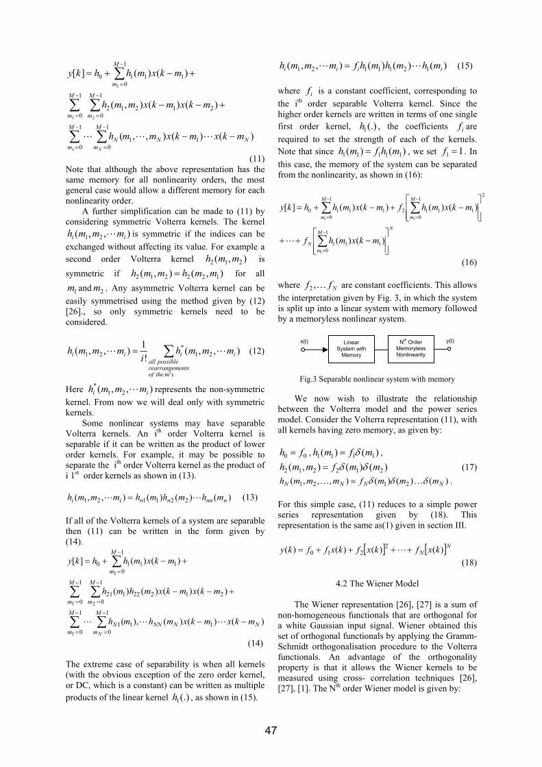
11

1

0

1

0

1

0

1

021212

1

01110

1

1 2

1

NN

M

m

M

mN

M

m

M

m

M

m

mkxmkxmmh

mkxmkxmmh

mkxmhhky

N

−−

+−−

+−+=

∑ ∑

∑ ∑

∑

−

=

−

=

−

=

−

=

−

=

LLL

(11) Note that although the above representation has the same memory for all nonlinearity orders, the most general case would allow a different memory for each nonlinearity order. A further simplification can be made to (11) by considering symmetric Volterra kernels. The kernel

),,( 21 ii mmmh L is symmetric if the indices can be exchanged without affecting its value. For example a second order Volterra kernel ),( 212 mmh is symmetric if ),(),( 122212 mmhmmh = for all

1m and 2m . Any asymmetric Volterra kernel can be easily symmetrised using the method given by (12) [26]., so only symmetric kernels need to be considered.

∑=

smtheofentsrearrangem

possiblealliiii mmmh

immmh

'

21*

21 ),,(!

1),,( LL (12)

Here ),,( 21*

ii mmmh L represents the non-symmetric kernel. From now we will deal only with symmetric kernels. Some nonlinear systems may have separable Volterra kernels. An ith order Volterra kernel is separable if it can be written as the product of lower order kernels. For example, it may be possible to separate the ith order Volterra kernel as the product of i 1st order kernels as shown in (13).

)()()(),,( 221121 nnnnnii mhmhmhmmmh LL = (13) If all of the Volterra kernels of a system are separable then (11) can be written in the form given by (14).

)()()(),(

)()()()(

)()(][

11

1

0

1

01

1

0

1

021222121

1

01110

1

1 2

1

NNNN

M

m

M

mN

M

m

M

m

M

m

mkxmkxmhmh

mkxmkxmhmh

mkxmhhky

N

−−

+−−

+−+=

∑ ∑

∑ ∑

∑

−

=

−

=

−

=

−

=

−

=

LLL

(14) The extreme case of separability is when all kernels (with the obvious exception of the zero order kernel, or DC, which is a constant) can be written as multiple products of the linear kernel (.)1h , as shown in (15).

)()()(),,( 1211121 iiii mhmhmhfmmmh LL = (15) where if is a constant coefficient, corresponding to the ith order separable Volterra kernel. Since the higher order kernels are written in terms of one single first order kernel, (.)1h , the coefficients if are required to set the strength of each of the kernels. Note that since )()( 11111 mhfmh = , we set 11 =f . In this case, the memory of the system can be separated from the nonlinearity, as shown in (16):

NM

mN

M

m

M

m

mkxmhf

mkxmhfmkxmhhky

⎥⎥⎦

⎤

⎢⎢⎣

⎡−++

⎥⎥⎦

⎤

⎢⎢⎣

⎡−+−+=

∑

∑ ∑

−

=

−

=

−

=

1

0111

21

0

1

011121110

1

1 1

)()(

)()()()(][

L

(16)

where Nff K,2 are constant coefficients. This allows the interpretation given by Fig. 3, in which the system is split up into a linear system with memory followed by a memoryless nonlinear system.

Fig.3 Separable nonlinear system with memory

We now wish to illustrate the relationship between the Volterra model and the power series model. Consider the Volterra representation (11), with all kernels having zero memory, as given by:

00 fh = , )()( 1111 mfmh δ= , )()(),( 212212 mmfmmh δδ= (17)

)()()(),,,( 2121 NNNN mmmfmmmh δδδ KK = . For this simple case, (11) reduces to a simple power series representation given by (18). This representation is the same as(1) given in section III.

[ ] [ ]NN kxfkxfkxffky )()()()( 2210 ++++= L

(18)

4.2 The Wiener Model

The Wiener representation [26], [27] is a sum of non-homogeneous functionals that are orthogonal for a white Gaussian input signal. Wiener obtained this set of orthogonal functionals by applying the Gramm-Schmidt orthogonalisation procedure to the Volterra functionals. An advantage of the orthogonality property is that it allows the Wiener kernels to be measured using cross- correlation techniques [26], [27], [1]. The Nth order Wiener model is given by:

y(t)Linear System with

Memory

x(t) Nth Order Memoryless Nonlinearity

47

)](;[)](;[)](;[)](;[)( 1100

txkKtxkKtxkKtxkKty

NN

ii

L

L +++=

(19) where: - the ith order Wiener operator is referred to as

[.]iK ;

- 0)](;[)](;[ =txkKtxkK jjii for ji ≠ and

. denotes averaging. The significance of the kernels ki will emerge in the following discussion. Continuous time expressions for the Wiener functionals up to third order are given below:

000 )](;[ ktxkK = (20)

∫∞

−=0

111111 )()()](;[ τττ dtxktxkK (21)

∫ ∫∞∞

−−=0 0

212121222 ))((),()](;[ ττττττ ddttxktxkK

(22)

210

122132

310

31321333

)(),,(3

)()(),,()](;[

ττττττσ

τττττττ

ddtxk

ddtxtxktxkK

∫∫

∫∫∫−−

−−= LL

(23) As with the Volterra model, discrete time versions of the above can be easily written by following the method used for the Volterra representations. Also, a Wiener truncated order and memory can be obtained by following the same procedure as foe the Volterra case. A Wiener model that uses symmetric Wiener kernels can also be derived, but it is a little more involved than the symmetrised Volterra representation because of the non-homogenity of the Wiener functionals. For example a 3rd order discrete time Wiener model with symmetric kernels can be written as:

)](;[)](;[)](;[)](;[)(

3322

1100

nxkKnxkKnxkKnxkKny

+++=

(24)

where:

000 )](;[ knxkK = (25)

∑−

=

−=1

011111

1

)()()](;[M

mmnxmknxkK (26)

∑ ∑−

=

−

=

−−=1

0

1

21212221 12

)()(),()](;[M

m

M

mmmnxmnxmmknxkK

(27)

)()(),,(

)(),,(3)()(

)(),,()](;[

2

1

0

1

012213

2

1

011113

222

1

0

1

0

1

01321333

112

2

1

1 2 3

mnxmnxmmmk

mnxmmmkmnxmnx

mnxmmmknxkK

M

m

M

mmm

M

m

M

m

M

m

M

m

−−−

−−−−

−=

∑ ∑

∑

∑ ∑∑

−

=

−

≠=

−

=

−

=

−

=

−

=

σ

σ

(28) Also, in the same way as the Volterra model can be compared to the power series model, the Wiener model can be compared to its memoryless counterpart, the Hermite polynomial representation It is easy to show that if memoryless Wiener kernels are substituted in equations (21) –(23), the Wiener functionals degenerate to Hermite polynomials. Although the main advantage of the orthogonality property is that it allows simple Wiener kernel measurement by cross-correlation approach, there are other benefits related to the orthogonality of the model. For example, the orthogonality property may also lead to improved convergence compared to the Volterra model. Higher order models entail a high computational burden. So, often, we choose or are forced to use a Volterra or Wiener representation of lower nonlinearity order than the system to be modeled. Under the appropriate continuity conditions, either a finite order Volterra or Wiener representation will give an arbitrary degree of accuracy (generalized Weierstrass theorem). However, there is a significant difference between using the Volterra and Wiener models. The values of the Volterra kernels will depend on the order of the Volterra representation being used. If the order of the Volterra model is change, The Volterra kernels will change, and they must be recalculated. If the order of the Volterra representation reaches the actual system order, any further increase in the Volterra representation order would not cause the Volterra kernels to change. However, the completeness property of the orthogonal Wiener model gives the following advantage. For a Wiener model of order N, the Wiener kernels are always optimum in least mean squared error sense. If the Wiener model order is increased, the lower order Wiener kernels remain the same and do not have to be re-estimated. Only the additional higher order Wiener kernels need to bee measured. The completeness property also means that the ith order Wiener kernel contains higher than ith order information about the system. Therefore, an ith order Wiener model will contain higher order information than an ith order Volterra model. In some situations, one may need to derive Volterra kernels from a set of Wiener kernels, or Wiener kernels from a set of Volterra kernels. A set of Volterra model kernels up to Nth order may be obtained from a set of Wiener kernels up to Nth order, by using the relationships obtained from [26] and given below as (29)-(34). For the purpose of illustration we consider a third order case. The 0th

48

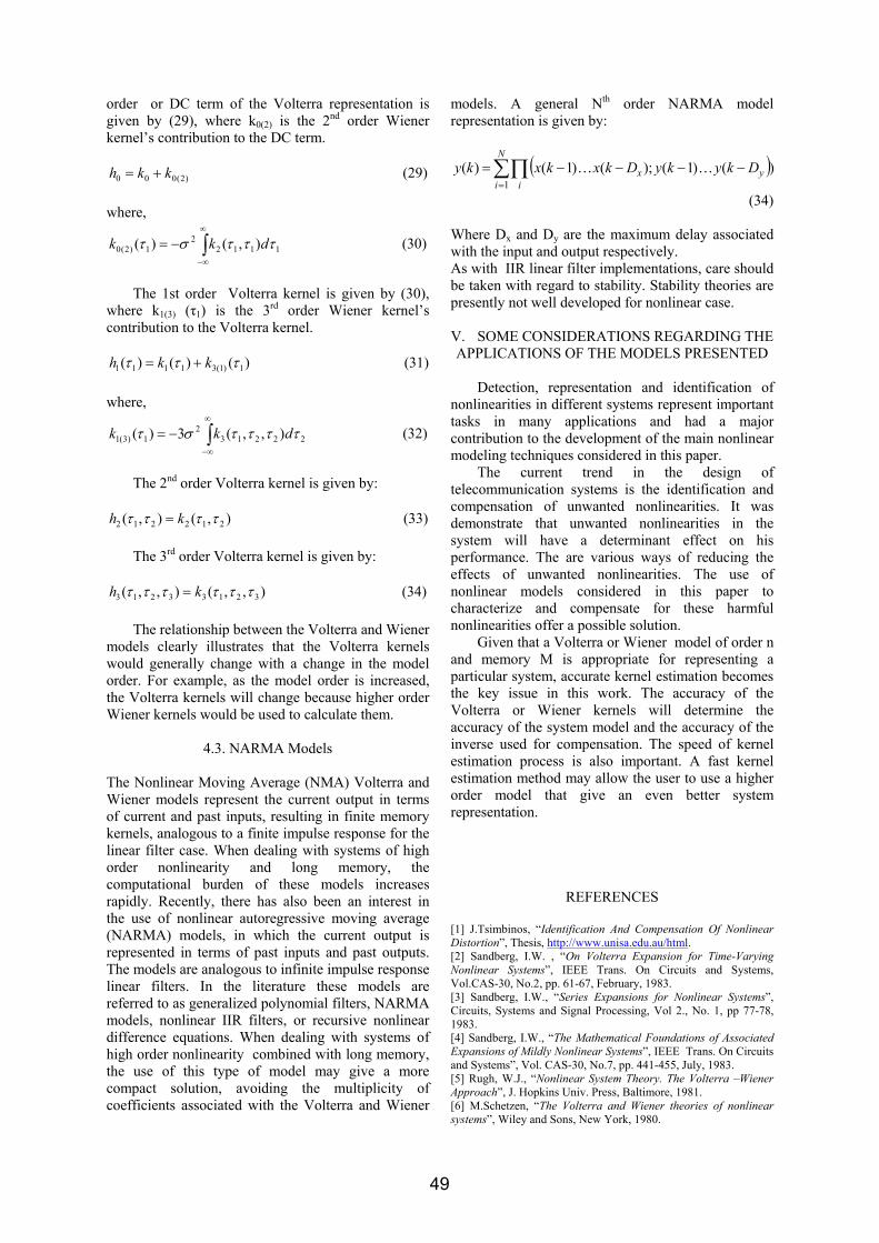
order or DC term of the Volterra representation is given by (29), where k0(2) is the 2nd order Wiener kernel’s contribution to the DC term.

)2(000 kkh += (29) where,

∫∞

∞−

−= 11122

1)2(0 ),()( τττστ dkk (30)

The 1st order Volterra kernel is given by (30), where k1(3) (τ1) is the 3rd order Wiener kernel’s contribution to the Volterra kernel.

)()()( 1)1(31111 τττ kkh += (31) where,

∫∞

∞−

−= 222132

1)3(1 ),,(3)( ττττστ dkk (32)

The 2nd order Volterra kernel is given by:

),(),( 212212 ττττ kh = (33) The 3rd order Volterra kernel is given by:

),,(),,( 32133213 ττττττ kh = (34) The relationship between the Volterra and Wiener models clearly illustrates that the Volterra kernels would generally change with a change in the model order. For example, as the model order is increased, the Volterra kernels will change because higher order Wiener kernels would be used to calculate them.

4.3. NARMA Models

The Nonlinear Moving Average (NMA) Volterra and Wiener models represent the current output in terms of current and past inputs, resulting in finite memory kernels, analogous to a finite impulse response for the linear filter case. When dealing with systems of high order nonlinearity and long memory, the computational burden of these models increases rapidly. Recently, there has also been an interest in the use of nonlinear autoregressive moving average (NARMA) models, in which the current output is represented in terms of past inputs and past outputs. The models are analogous to infinite impulse response linear filters. In the literature these models are referred to as generalized polynomial filters, NARMA models, nonlinear IIR filters, or recursive nonlinear difference equations. When dealing with systems of high order nonlinearity combined with long memory, the use of this type of model may give a more compact solution, avoiding the multiplicity of coefficients associated with the Volterra and Wiener

models. A general Nth order NARMA model representation is given by:

( ))()1();()1()(1∑∏=

−−−−=N

i iyx DkykyDkxkxky KK

(34) Where Dx and Dy are the maximum delay associated with the input and output respectively. As with IIR linear filter implementations, care should be taken with regard to stability. Stability theories are presently not well developed for nonlinear case. V. SOME CONSIDERATIONS REGARDING THE APPLICATIONS OF THE MODELS PRESENTED

Detection, representation and identification of nonlinearities in different systems represent important tasks in many applications and had a major contribution to the development of the main nonlinear modeling techniques considered in this paper. The current trend in the design of telecommunication systems is the identification and compensation of unwanted nonlinearities. It was demonstrate that unwanted nonlinearities in the system will have a determinant effect on his performance. The are various ways of reducing the effects of unwanted nonlinearities. The use of nonlinear models considered in this paper to characterize and compensate for these harmful nonlinearities offer a possible solution. Given that a Volterra or Wiener model of order n and memory M is appropriate for representing a particular system, accurate kernel estimation becomes the key issue in this work. The accuracy of the Volterra or Wiener kernels will determine the accuracy of the system model and the accuracy of the inverse used for compensation. The speed of kernel estimation process is also important. A fast kernel estimation method may allow the user to use a higher order model that give an even better system representation.

REFERENCES [1] J.Tsimbinos, “Identification And Compensation Of Nonlinear Distortion”, Thesis, http://www.unisa.edu.au/html. [2] Sandberg, I.W. , “On Volterra Expansion for Time-Varying Nonlinear Systems”, IEEE Trans. On Circuits and Systems, Vol.CAS-30, No.2, pp. 61-67, February, 1983. [3] Sandberg, I.W., “Series Expansions for Nonlinear Systems”, Circuits, Systems and Signal Processing, Vol 2., No. 1, pp 77-78, 1983. [4] Sandberg, I.W., “The Mathematical Foundations of Associated Expansions of Mildly Nonlinear Systems”, IEEE Trans. On Circuits and Systems”, Vol. CAS-30, No.7, pp. 441-455, July, 1983. [5] Rugh, W.J., “Nonlinear System Theory. The Volterra –Wiener Approach”, J. Hopkins Univ. Press, Baltimore, 1981. [6] M.Schetzen, “The Volterra and Wiener theories of nonlinear systems”, Wiley and Sons, New York, 1980.

49

[7]Lin, J.N., Unbehaunen, R., “2-D Adaptive Volterra Filter for 2-D Nonlinear Channel Equalization and Image Restoration”, Electron. Letters, Vol.28, No.2, pp. 180-182, Jan., 1992. [8] Gin-Kou Ma, Junghsi Lee, Mathews V.J., “A RLS Bilinear Filter for Channel Equalization”, IEEE Proceedings, Vol. III, pp. 257-260, 1994. [9] Bellafemina M., Benedetto S., ”Identification and Equalization of Nonlinear Channels for Digital Transmission”, Proc. IEEE Int. Symp. Circuits and Systems, pp. 1477-1480, 1985. [10] Giannakis, G.B., Serpedin, E., “Linear Multichannel Blind Equalizers of Nonlinear FIR Volterra Channels”, IEEE Trans. On Signal Processing, Vol. 45, No. 1, pp. 67-81, Jan., 1997. [11] Prakriya, S., Hatzianakos, “Blind identification of LTI-ZMNL-LTI Nonlinear Channel Models”, IEEE Trans. Signal Processing, Vol. 43, pp 3007-3013, Dec., 1995. [12] Grohan, P., Marcos, S., “ Limits and Cures of Nonlinear Channel Equalization by Polynomial Filters”, NSIP 95, http://poseidon.csd.auth.gr/HEADER/Internal/Workshop/papers/p_15_2.html. [13] Perry, A., “A Tutorial On The Origin and Control of Echo in Telecommunications Systems”, NMS Communications, http://www.nmscommunications.com [14] Stenger, A., Kellermann, W., Rabenstein, R., “Adaptation of Acoustic Echo Cancellers Incorporating a Memoryless Nonlinearity”, IEEE Work Shop on Acoustic Echo and Noise Control” (IWAENC’99), Pacono Manor, USA, 1992, stenger@nt.e-technik.uni-erlangen.de [15] Stenger, A., Rabenstein, R., “Adaptive Volterra Filters for Nonlinear Acoustic Echo Cancellation”, Proc. NSIP’99, Antalya, Turkey, Jun., 1999, stenger@nt.e-technik.uni-erlangen.de [16] Stenger, A., Kellermann, W., “ Nonlinear Acoustic Echo Cancellation with Fast Converging Memoryless Preprocessor”, Proceedings of the ICASSP 2000, pp. 805-809, Istanbul, Turkey, 2000. [17] Stenger, A., Kellermann, W., “Adaptation of a Memoryless Preprocessor for Nonlinear Acoustic Echo Canceling”, Signal Processing 80, No.9, pp. 1747-1760, 2000. [18] Stenger, A., Kellermann, W., “RLS-Adapted Polynomial for Nonlinear Acoustic Echo Canceling”, Proceedings of the EUSIPCO 2000, pp. 1867-1870, Tampere, Finland, 2000. [19] Korenberg, M., Hunter, I., “,The Identification of Nonlinear Biological Systems: Wiener Kernel Approaches”, Annals of Biomedical Engineering, Vol.18,pp. 629-654,1990. [20] Marmarelis, V.Z., “Identification of Nonlinear Biological Systems using Laguerre Expansion of Kernels”, Annals of Biomedical Engineering, Vol. 21., pp. 573-589, 1999. [21]Chon, Ki H., Chen, Yu-Ming, Holstein-Rathlou, Marmarelis, V.Z., “Nonlinear System Analysis of Renal Auto Regulation in Normotensive and Hypertensive Rats”, IEEE Trans. On Biomedical Engineering, Vol. 45., No. 3, pp 342-353. [22] Zhang, Q., et. al., “Factors Affecting Volterra Kernel Estimation: Emphasis on Lung Tissue Viscoelasticity”, Annals of Biomedical Engineering, Vol. 26., pp. 103-116, 1998. [23] Mc Rory, J.G. Johnson, R., “Volterra Kernel Estimation for Mildly Nonlinear Amplifiers”, Electronic Letters, Vol. 29, No.23, pp. 2007-2008, 1993. [24] Pitas, I., Venetsanopoulos, A.N., “Nonlinear Digital Filters Principles and Applications” Kluwer Academic Publisher, Boston/ Dordrecht/ London, 1990. [25] ] Koh, T., Powers, E., J., “Second Order Volterra Filtering and its Application to Nonlinear System Identification” IEEE Trans on ASSP, Vol. ASSP-33, No. 6, pag.1445-1455, decembrie 1985. [26] Schetzen, M., “The Volterra and Wiener theories of nonlinear systems”, Wiley and Sons, New York, 1980 [27] Wiener, N., “Nonlinear Problems in Random Theory”, The Technology Press of MIT and John Wiley and Sons, 1958.

50

Buletinul Ştiinţific al Universităţii "Politehnica" din Timişoara

Seria ELECTRONICĂ şi TELECOMUNICAŢII TRANSACTIONS on ELECTRONICS and COMMUNICATIONS

Tom 48(62), Fascicola 1, 2003

Neural Networks Intelligent Tools For Telecommunications Problems

Corina Botoca1, Georgeta Budura

1 Facultatea de Electronică şi Telecomunicaţii, Departamentul Comunicaţii Bd. V. Pârvan Timişoara 1900 e-mail corinab@etc.ee.utt.ro

Abstract: Neural Networks are nonlinear dynamic systems able to offer a solution almost anywhere classic methods have failed. This paper gives an overview of the applications of neural networks in telecommunications. There are presented the relevant characteristics that recommend neural networks as elegant and reliable tools for complex telecommunications problems. There are exposed some of the training algorithms. The conclusions highlight the difficulties that may arise in using neural networks. Key words: neural networks, training algorithm, neuron, telecommunication applications

I.INTRODUCTION

Intelligence is defined as the ability to adapt to new situations, to solve ongoing problems on the basis of acquired experience (dictionary). In computer engineering the significance of the term intelligence is still of actual debate. One thing is clear: intelligence implies the capability of deriving useful data from the stored information, to change the behavior without the intervention of a user.

There are two distinctive directions of developing artificial intelligence: • On the basis of efficient soft programs using

traditional computers; • On the basis of a brand new architecture, trying to

model the human brains processing; In the first direction it is important to achieve the

proposed task in the most secure and efficient way, without trying to model the human methods and techniques of knowledge processing. It includes all rule-based methods such as artificial intelligence, fuzzy logic and genetic algorithms.

Anywhere the conventional formalism has failed due to the combinatorial explosion and the long processing time caused by the sequentiallity of operation, neural networks offer a new frame for knowledge processing. A NN is a computer architecture soft , hard or both models, that works on the way that human brains process sensory stimuli. NN is a non rule-based technique and can be made stochastic, so the same action does not necessary take place each time for the same input. A stochastic behavior allows to a NN to fully explore its environment and potentially to find a better solution than all other methods.

There have been conceived many definitions for NN, one of them of Haykin [17], a personality in this field, is following: "A neural network is a massively parallel distributed processor that has a natural propensity for storing experiential knowledge and making it available for use. It resembles the brain in two respects: 1.Knowledge is acquired by the network through a learning process. 2.Interneuron connection strengths known as synaptic weights are used to store the knowledge" NN take a great amount of information and draw all at once a conclusion, not as a traditional computer in deductive consecutive steps. Some training data are fed into the NN and it learns by modifying its parameters in order to find the correct answer. The more data fed into a NN the better the results (it’s not the case of a conventional computer).

II THE ARGUMENTS OF NEURAL NETWORKS USE

The characteristics of NN are also argu-ments of

using them in complex problems of telecommunications: Learning from examples Learning is the ability of NN to modify their parameters, improving their performance, in order to minimize a cost function. In general learning is stopped according to given criteria (e.g. when the obtained weights produce a sufficiently small error performance). Adaptability is closely related with learning and it is indispensable when the NN operates in a nonstationary environment.

From this point of view there are two types of NN: • with fixed weights , when the weights are

modified during a first phase of processing (named learning or training) and than "frizzed" at the final values obtained (that are used during operation);

• with adaptable weights, when learning continues also during the phase of functioning (" on line" learning) ;

51

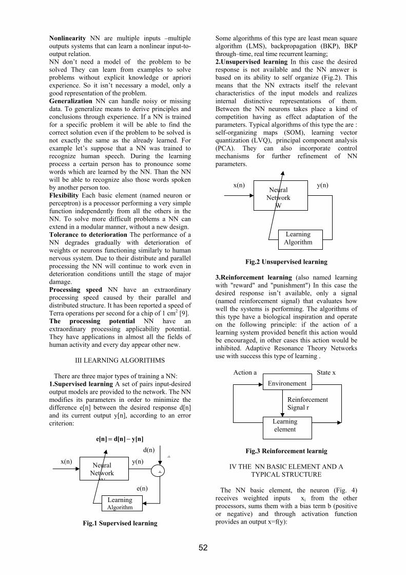
Nonlinearity NN are multiple inputs –multiple outputs systems that can learn a nonlinear input-to-output relation. NN don’t need a model of the problem to be solved They can learn from examples to solve problems without explicit knowledge or apriori experience. So it isn’t necessary a model, only a good representation of the problem. Generalization NN can handle noisy or missing data. To generalize means to derive principles and conclusions through experience. If a NN is trained for a specific problem it will be able to find the correct solution even if the problem to be solved is not exactly the same as the already learned. For example let’s suppose that a NN was trained to recognize human speech. During the learning process a certain person has to pronounce some words which are learned by the NN. Than the NN will be able to recognize also those words spoken by another person too. Flexibility Each basic element (named neuron or perceptron) is a processor performing a very simple function independently from all the others in the NN. To solve more difficult problems a NN can extend in a modular manner, without a new design. Tolerance to deterioration The performance of a NN degrades gradually with deterioration of weights or neurons functioning similarly to human nervous system. Due to their distribute and parallel processing the NN will continue to work even in deterioration conditions untill the stage of major damage. Processing speed NN have an extraordinary processing speed caused by their parallel and distributed structure. It has been reported a speed of Terra operations per second for a chip of 1 cm2 [9]. The processing potential NN have an extraordinary processing applicability potential. They have applications in almost all the fields of human activity and every day appear other new.

III LEARNING ALGORITHMS

There are three major types of training a NN: 1.Supervised learning A set of pairs input-desired output models are provided to the network. The NN modifies its parameters in order to minimize the difference e[n] between the desired response d[n] and its current output y[n], according to an error criterion:

]n[y]n[d]n[e −=

Fig.1 Supervised learning

Some algorithms of this type are least mean square algorithm (LMS), backpropagation (BKP), BKP through–time, real time recurrent learning; 2.Unsupervised learning In this case the desired response is not available and the NN answer is based on its ability to self organize (Fig.2). This means that the NN extracts itself the relevant characteristics of the input models and realizes internal distinctive representations of them. Between the NN neurons takes place a kind of competition having as effect adaptation of the parameters. Typical algorithms of this type the are : self-organizing maps (SOM), learning vector quantization (LVQ), principal component analysis (PCA). They can also incorporate control mechanisms for further refinement of NN parameters.

Fig.2 Unsupervised learning

3.Reinforcement learning (also named learning with "reward" and "punishment") In this case the desired response isn’t available, only a signal (named reinforcement signal) that evaluates how well the systems is performing. The algorithms of this type have a biological inspiration and operate on the following principle: if the action of a learning system provided benefit this action would be encouraged, in other cases this action would be inhibited. Adaptive Resonance Theory Networks use with success this type of learning .

Fig.3 Reinforcement learnig

IV THE NN BASIC ELEMENT AND A

TYPICAL STRUCTURE

The NN basic element, the neuron (Fig. 4) receives weighted inputs xi from the other processors, sums them with a bias term b (positive or negative) and through activation function provides an output x=f(y):

Neural Network

W

x(n) y(n)

Learning Algorithm

Neural Network

W

x(n) y(n)

Learning Algorithm

d(n)

e(n)

+

++

Environement

Learning element

Reinforcement Signal r

Action a State x

52

∑=

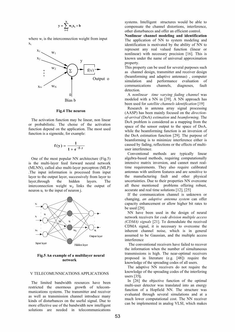
+=N

1iii bxwy

where wi is the interconnection weight from input xi.

Fig.4 The neuron

The activation function may be linear, non linear

or probabilistic. The choise of the activation function depend on the application. The most used function is a sigmoide, for example:

y.e11)y(f

β−+=

One of the most popular NN architecture (Fig.5)

is the multi-layer feed forward neural network (MLNN), called also multi-layer perceptron (MLP) .The input information is processed from input layer to the output layer, successively from layer to layer,through the hidden layers. The interconnection weight wji links the output of neuron ui to the input of neuron j.

Input layer Hidden layer

Output layer

x1

xi

xN

ui

uk

wji

···

··· ·

·uj

wkj

···

Fig.5 An example of a multilayer neural network

V TELECOMUNNICATIONS APPLICATIONS

The limited bandwidth resources have been

restricted the enormous growth of telecom-munications systems. The transmitter and receiver as well as transmission channel introduce many kinds of disturbances on the useful signal. Due to more effective use of the bandwidth new intelligent solutions are needed in telecommunications

systems. Intelligent structures would be able to compensate the channel distortions, interference, other disturbances and offer an efficient control. Nonlinear channel modeling and identification The application of NN to system modeling and identification is motivated by the ability of NN to represent any real valued function (linear or nonlinear) with necessary precision [16]. This is known under the name of universal approximation property. This property can be used for several purposes such as channel design, transmitter and receiver design (beamforming and adaptive antennas) , computer simulation and performance evaluation of communications channels, diagnoses, fault detection.

A nonlinear time varying fading channel was modeled with a NN in [39]. A NN approach has been used for satellite channels identification [19]

Research in antenna array signal processing (AASP) has been mainly focused on the direction-of-arrival (DoA) estimation and beamforming. The DoA problem is considered as a mapping from the space of the sensor output to the space of DoA, while the beamforming function is an inversion of the DoA estimation function [29]. The purpose of beamforming is to minimize interference either is caused by fading, reflections or the effects of multi-user interference.

Conventional methods are typically linear algebra-based methods, requiring computationally intensive matrix inversion, and cannot meet real-time requirements. They also require calibrated antennas with uniform features and are sensitive to the manufacturing fault and other physical uncertainties. Due to their properties NN overcome all these mentioned problems offering robust, accurate and real time solutions [12], [25]

If the communication channel is unknown or changing, an adaptive antenna system can offer capacity enhancement or allow higher bit rates to be used [29].

NN have been used in the design of neural network receivers for code division multiple access (CDMA) signals [21]. To demodulate the received CDMA signal, it is necessary to overcome the inherent channel noise, which is in general assumed to be Gaussian, and the multiple access interference

The conventional receivers have failed to recover the information when the number of simultaneous transmissions is high. The near-optimal receivers proposed in literature (e.g. [48]) require the knowledge of the spreading codes of all users.

The adaptive NN receivers do not require the knowledge of the spreading codes of the interfering users [35].

In [26] the objective function of the optimal multi-user detector was translated into an energy function of a Hopfield NN. The structure was evaluated through several simulations and at a much lower computational cost. The NN receiver can be implemented in analog VLSI, which makes

Output o

xN

w1 x1

x2

Bias b

wN

Σ

y

f(y) w2

53

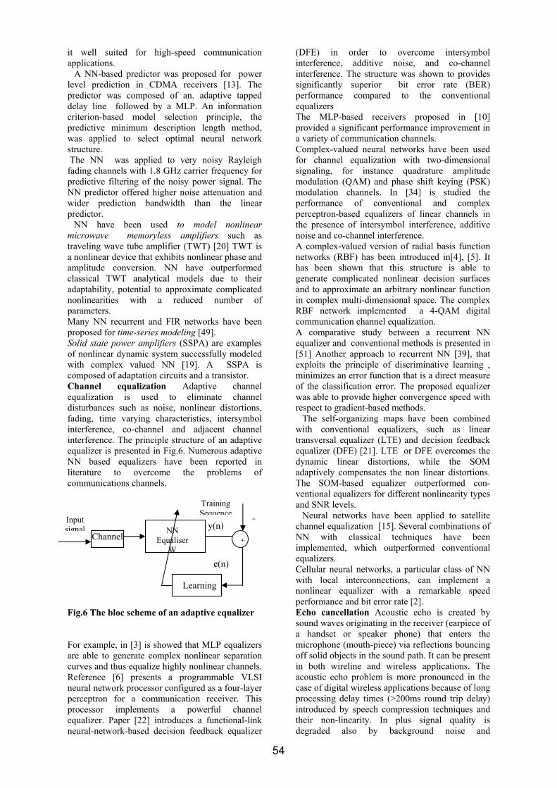
it well suited for high-speed communication applications.

A NN-based predictor was proposed for power level prediction in CDMA receivers [13]. The predictor was composed of an. adaptive tapped delay line followed by a MLP. An information criterion-based model selection principle, the predictive minimum description length method, was applied to select optimal neural network structure. The NN was applied to very noisy Rayleigh fading channels with 1.8 GHz carrier frequency for predictive filtering of the noisy power signal. The NN predictor offered higher noise attenuation and wider prediction bandwidth than the linear predictor.

NN have been used to model nonlinear microwave memoryless amplifiers such as traveling wave tube amplifier (TWT) [20] TWT is a nonlinear device that exhibits nonlinear phase and amplitude conversion. NN have outperformed classical TWT analytical models due to their adaptability, potential to approximate complicated nonlinearities with a reduced number of parameters. Many NN recurrent and FIR networks have been proposed for time-series modeling [49]. Solid state power amplifiers (SSPA) are examples of nonlinear dynamic system successfully modeled with complex valued NN [19]. A SSPA is composed of adaptation circuits and a transistor. Channel equalization Adaptive channel equalization is used to eliminate channel disturbances such as noise, nonlinear distortions, fading, time varying characteristics, intersymbol interference, co-channel and adjacent channel interference. The principle structure of an adaptive equalizer is presented in Fig.6. Numerous adaptive NN based equalizers have been reported in literature to overcome the problems of communications channels.

Fig.6 The bloc scheme of an adaptive equalizer For example, in [3] is showed that MLP equalizers are able to generate complex nonlinear separation curves and thus equalize highly nonlinear channels. Reference [6] presents a programmable VLSI neural network processor configured as a four-layer perceptron for a communication receiver. This processor implements a powerful channel equalizer. Paper [22] introduces a functional-link neural-network-based decision feedback equalizer

(DFE) in order to overcome intersymbol interference, additive noise, and co-channel interference. The structure was shown to provides significantly superior bit error rate (BER) performance compared to the conventional equalizers The MLP-based receivers proposed in [10] provided a significant performance improvement in a variety of communication channels. Complex-valued neural networks have been used for channel equalization with two-dimensional signaling, for instance quadrature amplitude modulation (QAM) and phase shift keying (PSK) modulation channels. In [34] is studied the performance of conventional and complex perceptron-based equalizers of linear channels in the presence of intersymbol interference, additive noise and co-channel interference. A complex-valued version of radial basis function networks (RBF) has been introduced in[4], [5]. It has been shown that this structure is able to generate complicated nonlinear decision surfaces and to approximate an arbitrary nonlinear function in complex multi-dimensional space. The complex RBF network implemented a 4-QAM digital communication channel equalization. A comparative study between a recurrent NN equalizer and conventional methods is presented in [51] Another approach to recurrent NN [39], that exploits the principle of discriminative learning , minimizes an error function that is a direct measure of the classification error. The proposed equalizer was able to provide higher convergence speed with respect to gradient-based methods.

The self-organizing maps have been combined with conventional equalizers, such as linear transversal equalizer (LTE) and decision feedback equalizer (DFE) [21]. LTE or DFE overcomes the dynamic linear distortions, while the SOM adaptively compensates the non linear distortions. The SOM-based equalizer outperformed con-ventional equalizers for different nonlinearity types and SNR levels.

Neural networks have been applied to satellite channel equalization [15]. Several combinations of NN with classical techniques have been implemented, which outperformed conventional equalizers. Cellular neural networks, a particular class of NN with local interconnections, can implement a nonlinear equalizer with a remarkable speed performance and bit error rate [2]. Echo cancellation Acoustic echo is created by sound waves originating in the receiver (earpiece of a handset or speaker phone) that enters the microphone (mouth-piece) via reflections bouncing off solid objects in the sound path. It can be present in both wireline and wireless applications. The acoustic echo problem is more pronounced in the case of digital wireless applications because of long processing delay times (>200ms round trip delay) introduced by speech compression techniques and their non-linearity. In plus signal quality is degraded also by background noise and

NN Equaliser

W

Input signal y(n)

Channel

Training Sequence

e(n)

+

++

Learning

54

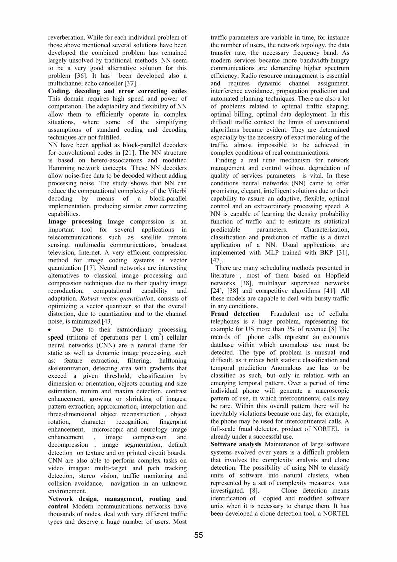
reverberation. While for each individual problem of those above mentioned several solutions have been developed the combined problem has remained largely unsolved by traditional methods. NN seem to be a very good alternative solution for this problem [36]. It has been developed also a multichannel echo canceller [37]. Coding, decoding and error correcting codes This domain requires high speed and power of computation. The adaptability and flexibility of NN allow them to efficiently operate in complex situations, where some of the simplifying assumptions of standard coding and decoding techniques are not fulfilled. NN have been applied as block-parallel decoders for convolutional codes in [21]. The NN structure is based on hetero-associations and modified Hamming network concepts. These NN decoders allow noise-free data to be decoded without adding processing noise. The study shows that NN can reduce the computational complexity of the Viterbi decoding by means of a block-parallel implementation, producing similar error correcting capabilities. Image processing Image compression is an important tool for several applications in telecommunications such as satellite remote sensing, multimedia communications, broadcast television, Internet. A very efficient compression method for image coding systems is vector quantization [17]. Neural networks are interesting alternatives to classical image processing and compression techniques due to their quality image reproduction, computational capability and adaptation. Robust vector quantization. consists of optimizing a vector quantizer so that the overall distortion, due to quantization and to the channel noise, is minimized.[43] • Due to their extraordinary processing speed (trilions of operations per 1 cm2) cellular neural networks (CNN) are a natural frame for static as well as dynamic image processing, such as: feature extraction, filtering, halftoning skeletonization, detecting area with gradients that exceed a given threshold, classification by dimension or orientation, objects counting and size estimation, minim and maxim detection, contrast enhancement, growing or shrinking of images, pattern extraction, approximation, interpolation and three-dimensional object reconstruction , object rotation, character recognition, fingerprint enhancement, microscopic and neurology image enhancement , image compression and decompression , image segmentation, default detection on texture and on printed circuit boards. CNN are also able to perform complex tasks on video images: multi-target and path tracking detection, stereo vision, traffic monitoring and collision avoidance, navigation in an unknown environement. Network design, management, routing and control Modern communications networks have thousands of nodes, deal with very different traffic types and deserve a huge number of users. Most

traffic parameters are variable in time, for instance the number of users, the network topology, the data transfer rate, the necessary frequency band. As modern services became more bandwidth-hungry communications are demanding higher spectrum efficiency. Radio resource management is essential and requires dynamic channel assignment, interference avoidance, propagation prediction and automated planning techniques. There are also a lot of problems related to optimal traffic shaping, optimal billing, optimal data deployment. In this difficult traffic context the limits of conventional algorithms became evident. They are determined especially by the necessity of exact modeling of the traffic, almost impossible to be achieved in complex conditions of real communications.

Finding a real time mechanism for network management and control without degradation of quality of services parameters is vital. In these conditions neural networks (NN) came to offer promising, elegant, intelligent solutions due to their capability to assure an adaptive, flexible, optimal control and an extraordinary processing speed. A NN is capable of learning the density probability function of traffic and to estimate its statistical predictable parameters. Characterization, classification and prediction of traffic is a direct application of a NN. Usual applications are implemented with MLP trained with BKP [31], [47].

There are many scheduling methods presented in literature , most of them based on Hopfield networks [38], multilayer supervised networks [24], [38] and competitive algorithms [41]. All these models are capable to deal with bursty traffic in any conditions. Fraud detection Fraudulent use of cellular telephones is a huge problem, representing for example for US more than 3% of revenue [8] The records of phone calls represent an enormous database within which anomalous use must be detected. The type of problem is unusual and difficult, as it mixes both statistic classification and temporal prediction Anomalous use has to be classified as such, but only in relation with an emerging temporal pattern. Over a period of time individual phone will generate a macroscopic pattern of use, in which intercontinental calls may be rare. Within this overall pattern there will be inevitably violations because one day, for example, the phone may be used for intercontinental calls. A full-scale fraud detector, product of NORTEL is already under a successful use. Software analysis Maintenance of large software systems evolved over years is a difficult problem that involves the complexity analysis and clone detection. The possibility of using NN to classify units of software into natural clusters, when represented by a set of complexity measures was investigated. [8]. Clone detection means identification of copied and modified software units when it is necessary to change them. It has been developed a clone detection tool, a NORTEL

55

product, which proved to be very useful in examination of the PROTEL soft system. Consumer products These products have already the capability of high-speed communications. This requires low cost and low power electronics. However, the domestic environment may not be radio frequency friendly so intelligent and adaptive receiver may improve the throughput without requiring an increase in transmitter power.

VI DESADVANTAGES

Although NN have proved the capability to solve many difficult problems, a critical analyses reveals some drawbacks: • NN is a "black box" – it doesn’t explain its

decisions. Deriving behavior rules seems inherent difficult.

• It’s a fact that NN can handle large numbers of variables and parameters. But data acquisition, relevant selection of variables is a difficult and time-consuming task. Data are normally pre-processed or parameterized before being presented to a NN. In this designing phase expertise in the field of the problem to be solved is necessary and invaluable.

• There are not clear construction rules concerning the best NN architecture for a given application (e.g. number of layers, number of neurons on a layer, type of network, with or without feedback) .The most used method in NN design is "trial and error".

• There is an art in choosing also the best method of learning, since if an inappropriate method is chosen the networks’ weights might not converge at all during training.

• The obtained NN configuration is appropriate only to a particular application, adaptation to another application is very difficult.

• Usually the NN configuration results in a massive structure, with many interconnections, of higher order, that can create difficulties in hard implementation. Repairing is practically impossible, because the operation is distributed in the whole NN structure and identification of broken component is not possible.

• It has become apparent that the task of moving from a successful, NN based prototype to a full applicable system is quite difficult.

VII CONCLUSIONS

This paper gives an overview of the applications

of NN in telecommunications. The exponentially growing number of papers in recent years show the great interest of researchers to neural based communications systems. A lot of successful products already developed show that NN can provide a powerful tool for telecommunications industry.

As one of the experts in NN concluded [50]: "NN can determine relationships between things you didn’t even know existed and will reveal hidden truths about your business".

Modern communications with their complex problems are quite the field recommended for NN applications. As conclusions, NN may offer solutions: • where a conventional process is not suitable,

can’t be easy defined or cannot fully capture the complexity in the data;

• where stochastic behavior is important, where an explanation of the NN decision is not required; NN will certainly be one of the key technologies

in the 21st century, so it is expected to concentrate a special effort of world research community. A rapid evolution has had recently the merging research field between all intelligent techniques : NN, genetic algorithms, fuzzy and expert systems. Hybrid intelligent systems will offer better, robust solutions implying a greater intelligence coefficient.

VIII REFERENCES [1] B. Baykal, A. Constantinides, "A Neural Network Approach to the Underdetermined Order Recursive Least-squares Adaptive Filtering", Neural Networks vol.10, no.8 1997, pp.1523-1531. [2] Corina Botoca, Georgeta Budura, “Using Cellular Neural Network To Adaptive Equalization”, Proceedings of the Symposium on Electronics and Telecommunications, ETC.2000, pp.245-249 [3] S. Chen, G. Gibson, C. Cowan, P. Grant, "Adaptive Equalization of Finite Non-linear Channels Using Multilayer Perceptron", Signal Processing 20, 1990, pp.107-119. [4] S. Chen, S. McLaughlin, B. Mulgrew, "Complex-valued radial basis function networks, Part I: Network Architecture and Learning Algorithms", Signal Processing 35, January, 1994, pp.19-31 [5] S. Chen, S. McLaughlin, B. Mulgrew, "Complex-valued Radial Basis Function Networks, Part II: Application to Digital Communication Channel Equalization", Signal Processing, 36, March, 1994, pp. 175-188 [6]J.Choi, S. Bang, B. Sheu, "A Programmable Analog VLSI Neural Network processor for Communication Receivers", IEEE Trans. Neural Networks ,May, 1993, pp. 484-495. [7] J.M.Cioffi, Limited-Precision Effects in Adaptive Filtering, IEEE Transactions On Circuits And Systems, vol. Cas-34, no. 7, July, 1987, pp.821-833 [8] T.Clarkson, "Applications of Neural Networks in Telecommunications" , 2002 [9]L.Chua, T.Roska, " Cellular Neural Network and Visual Computing - Foundations and Applications", Cambridge University Press, 2001 [10] G. De Veciana, A. Zakhor, "Neural Net-based Continuous Phase Modulation Receivers" , IEEE Trans. Communications, 40 August, 1992 [11] C.Douligeris, G.Develekos, "Neurofuzzy Control In ATM Networks", IEEE Communi-cations Magazine, May, 1997, pp.154-162 [12] Dorffner, 1999, Internal Report for NeuroNet, http://klc.ac.uk/neuronet/ [13] X.M. Gao, X.Z. Gao, J. Tanskanen, S. Ovaska, "Power Prediction in Mobile Com-munication Systems Using an Optimal Neural Network Structure", IEEE Trans. Neural Networks 8,November,1997. [14] G.J. Gibson, S. Siu, C. F. N. Cowan, “The Application of Nonlinear Structures to The Reconstruction of Binary Signals” ,vol. 39, no. 8, August, 1991 [15] A. Guntsch, M. Ibnkahla, G. Losquadro, M. Mazzella, D.Roviras, A. Timm, "EU's R&D Activities on Third Generation Mobile Satellite Systems ", IEEE Communications Magazine, February, 1998 [16] S. Haykin, L. Li, "Non Linear Adaptive Prediction of Nonstationary Signals", IEEE Trans. Signal Processing, 1995, pp.526-535

56

[17] S.Haykin “Neural Networks” Mcmillan Publishing Co., Englewood Cliffs, 1994 [18 ] Hecht-Nielsen "Neurocomputing" Addison-Wesley Publishing Company, 1990 [19] M. Ibnkahla, N.J. Bershad, J. Sombrin, F. CastanieH , "Neural Network Modeling and Identification of Non-linear Channels with Memory: Algorithms, Applications and Analytic models, IEEE Trans. Signal Process. ,May 1998, pp.1208-1220. [20] M. Ibnkahla, J. Sombrin, F. CastanieH , N.J. Bershad, "Neural Networks for Modeling Non-linear Memoryless Communication Channels", IEEE Trans. Commun.7, July, 1997, pp.768-771 [21] M. Ibnkahla, "Applications of Neural Networks to Digital Communication a Survey" IEEE Signal Processing Magazine,November, 1997, pp.1186-1215 [22] A. Hussain, J. Soraghan, T. Durrani, A New Adaptive Functional-link Neural Network-based DFE for Overcoming Co-channel Interference, IEEE Trans. Commun. 11, November, 1997,pp. 1358-1362 [23] J. Hwang, S. Kung, M. Niranjan, J. Principe, "The Past, Present, and Future of Neural Networks for Signal Processing",IEEE Signal Process. Mag, November, 1997, pp.28-48 [24] S.Jagannathan, A.Tohmaz, J.Talluri, "Congestion Control of ATM Networks Using a Learning Methodology," Proceedings of 2001 IEEE International Conference on Control Applications [25]Kartaloupoulus , 1999, Internal Report for IEEE Communications Society, http://www.comsoc.org/ [26] G. Kechriotis, E. Manolakos, "Hopfield Neural Network Implementation of The Optimal CDMA Multiuser Detector", IEEE Trans. Neural Networks,1,January,1996, pp.131-141. [27]B.Kosko "Neural Networks and Fuzzy Systems",Prentice Hall, Englewood Cliffs, NJ,1992 [28] B.Kosko "Neural Networks for Signal Processing, Prentice Hall, Englewood Cliffs, NJ, 1992 [29] A.K.Y.Lai, K.K.M.Cheng M.N.S.Swamy "Neural Methods For Antenna Array Signal Processing: A Review", Signal Processing Magazine, 2002, www.elsevier.com/locate/sigpro [30] J.Lee, Ch.Beach, N.Tepedelenloiglu, A Practical Radial Basis Function Equalizer, IEEE Transactions on Neural Networks, vol10,nr.2,pp.450-455, march, 1999 [31] N Leitao, L.Ahmeida, "Neural Networks In BIDN Flow Control:ATM Traffic Prediction Or Network Modeling", IEEE Communications Mag,October,1995, pp.50-56 [32] R.Logeswaran, "Transmission Issues of Artificial Neural Networks in a Prediction/ Based Lossless Data Compression Scheme", Proceedings IEEE ICT, 2001, pp.578-583, [33] Lester, S.H.Ngi, "Efficient Training of Neural Nets for Nonlinear Adaptive Filtering Using a Recursive Levenberg–Marquardt Algorithm", IEEE Transactions On Signal Processing, vol. 48, no. 7, July, 2000 [34] N. Lo, H. Hafez, "Neural Network Channel Equalization", Proceedings of International Joint Conference on Neural Networks , IJCNN'92, Vol. 2, 1992, pp. 981-986 [35] U. Mitra, V. Poor, "Adaptive Receiver Algorithms for Near-far Resistant CDMA", IEEE Transactions on Communications 43, February/March/April, 1995, pp.1713-1724 [36] M. Moonen, Y.Dologlou, G.Rombouts, "Combination Of Multimicrophone Echo And Noise Suppression Techniques For Enhancement Of Audio Signals", www.esat.kulueven.ac.be/sista/yearreport97 [37] M. Moonen, Y.Dologlou, G.Rombouts, "Adaptive Signal Processing Techniques For Long Acoustic Echo Cancellation And Hand-Free Teleconferencing", http://www.esat. kuleuven.ac.be/sista/yearreport97 [38] E.Nordstrom, J.Carlström, O.Gällmo, "Neural Networks For Adaptive Traffic Control In ATM Networks", IEEE Communications magazine, Vol33, No. 10, 1995, pp.43-49 [39] R. Parisi, E. Di Claudio, G. Orlandi, B. Rao, "Fast Adaptive Digital Equalization by Recurrent Neural Networks", IEEE Trans. Signal Process. 45, November, 1997, pp.2731-2739. [40] I. Popescu, I.Naforniţă, P. Constantinou, A. Kanatas, N. Moraitis, "Prediction of Outdoor Propagation Path Loss with Neural Networks", Proceedings of the 8th telecommunications Forum Telfor'2000, 21-23 November 2000, Belgrade, Serbia, pp. 140-143 [41] I.Reljin "Neural Network Based Low Cell Scheduler", Proceedings of 4th Neural Network Applications in Electrical Engineering, NEUREL’97, Belgrade, pp. 168-172

[42]B.Reljin, I.Reljin, "Neural Network In Telegraphic Control. Pro Et Contra ", IEEE Proceedings of 4th International Conference On Telecommunications In Modern Satellite Broadcasting, TELSIKS’99, pp 518-527,1999 [43] Seyed Bahram Zahir Azami, Gang Feng " Robust Vector Quantizer Design Using Self-Organizing Neural networks" Signal Proc. Magazine, 80, www.elsevier.com/locate/sigpro/, 2000 [44] L.M.San, J.Revuelta "A neuro-evolutionary framework for Bayesian blind equalization in digital communications " Signal Processing Magazine, 2002, www.elsevier.com/locate/sigpro [45]S.Sezer, Ph.Power, Neural Networks for High-Bandwidth QAM Channels, Proceedings IEEE ICT, 2001,pp.225-229 [46]Bertram E. Shi, Gabor-Type Filtering in Space and Time with Cellular Neural Networks, IEEE Transactions On Circuits And Systems—I: Fundamental Theory And Applications, vol. 45, no. 2, February, 1998,pp.121-132 [47]A.Taraff, I.Habib, T.Saadowi,"Intelligent Traffic Control For ATM Broadband Networks" , IEEE Communications Magazine, October,1995, pp. 76-82 [48] M. Varanasi, B. Aazhang, "Multistage Detection in Asynchronous Code-division Multiple Access Communications", IEEE Trans. Commun. 38, April, 1990,pp. 509-519. [49] H. Yu, S. Bang, "An Improved Time Series Prediction by Applying the Layer-by-layer Learning Method to FIR Neural Networks", Neural Networks 10, Nov,1997,pp.1717-1729. [50] "Making Brain Waves", CIO Magazine, January 1995, [http://www.cio.com] [51]"Time varying Channel Equalization", 2002, www.soma.mcmaster.ca/ASLWeb/Projects/ ChannelEqualization/

57

58

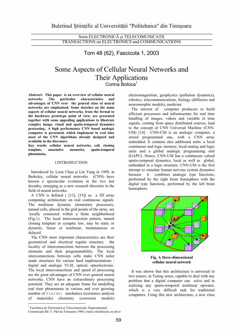
Buletinul Ştiinţific al Universităţii "Politehnica" din Timişoara

Seria ELECTRONICĂ şi TELECOMUNICAŢII TRANSACTIONS on ELECTRONICS and COMMUNICATIONS

Tom 48 (62), Fascicola 1, 2003

Some Aspects of Cellular Neural Networks and

Their Applications Corina Botoca1

1 Facultatea de Electronică şi Telecomunicaţii, Departamentul Comunicaţii Bd. V. Pârvan Timişoara 1900 e-mail corinab@etc.ee.utt.ro

Abstract: This paper is an overview of cellular neural networks .The particular characteristics and advantages of CNN over the general class of neural networks are emphasised. Some sketches on the main aspects of cellular neural networks, from the formal to the hardware prototype point of view, are presented together with some appealing applications to illustrate complex image, visual and spatio-temporal dynamics processing.. A high performance CNN based analogic computer is presented, which implement in real time most of the CNN algorithms already designed and available in the literature. Key words: cellular neural networks, cell, cloning template, associative memories, spatio-temporal phenomena,

I INTRODUCTION

Introduced by Leon Chua şi Lin Yang in 1988, at Berkeley, cellular neural networks (CNN) have known a spectacular evolution in the two last decades, emerging as a new research direction in the field of neural networks.

A CNN is defined ( [13], [15]) as a 3D array computing architecture on real continuous signals. The nonlinear dynamic elementary processors, named cells, placed in the grid points of the array, are locally connected within a finite neighborhood (Fig.1). The local interconnection pattern, named cloning template or synaptic law, may be static or dynamic, linear or nonlinear, instantaneous or delayed.

The CNN most important characteristics are their geometrical and electrical regular structure, the locality of interconnections between the processing elements and their programmability. The local interconnections between cells make CNN tailor made structures for various hard implementations : digital and analogic VLSI, optical, optoelectronic. The local interconnections and speed of processing are the great advantages of CNN over general neural networks. CNN have an extraordinary processing potential. They are an adequate frame for modelling real time phenomena in various and ever growing number of fields: mechanics (resistance analysis of materials) chemistry (corrosion models)

electromagnetism, geophysics (pollution dynamics), robotics, telecommunications, biology (diffusion and neuromorphic models), medicine.

The interest of computer producers to build efficient processors and infrastructure for real time handling of images, videos and variable in time signals, coming from space distributed sources, lead to the concept of CNN Universal Machine (CNN-UM) [14] . CNN-UM is an analogic computer, a stored programmed one, with a CNN array embedded. It contains also additional units: a local continuous and logic memory, local analog and logic units and a global analogic programming unit (GAPU). Hence, CNN-UM has a continuous valued spatio-temporal dynamics, local as well as global, embedded in a logic structure. CNN-UM is the first attempt to simulate human nervous system dynamics because it combines analogic type functions, performed by the right brain hemisphere with the digital type functions, performed by the left brain hemisphere.

Fig. A three-dimensional cellular neural network

It was shown that this architecture is universal in

two senses: in Turing sense, capable to deal with any problem that a digital computer can solve and in realizing any spatio-temporal nonlinear operator, which is a very difficult task for traditional computers. Using this new architecture, a new class

59

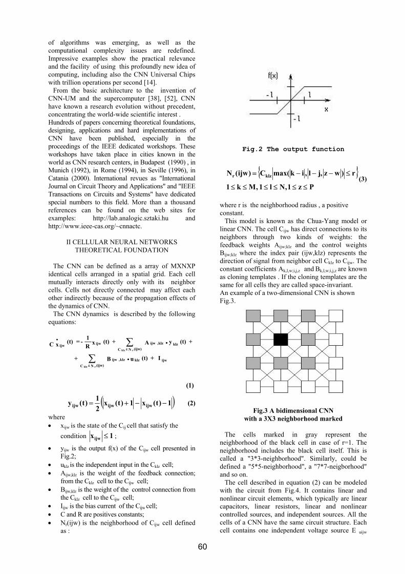
of algorithms was emerging, as well as the computational complexity issues are redefined. Impressive examples show the practical relevance and the facility of using this profoundly new idea of computing, including also the CNN Universal Chips with trillion operations per second [14].

From the basic architecture to the invention of CNN-UM and the supercomputer [38], [52], CNN have known a research evolution without precedent, concentrating the world-wide scientific interest . Hundreds of papers concerning theoretical foundations, designing, applications and hard implementations of CNN have been published, especially in the proceedings of the IEEE dedicated workshops. These workshops have taken place in cities known in the world as CNN research centers, in Budapest (1990) , in Munich (1992), in Rome (1994), in Seville (1996), in Catania (2000). International revues as "International Journal on Circuit Theory and Applications" and "IEEE Transactions on Circuits and Systems" have dedicated special numbers to this field. More than a thousand references can be found on the web sites for examples: http://lab.analogic.sztaki.hu and http://www.ieee-cas.org/~cnnactc.

II CELLULAR NEURAL NETWORKS THEORETICAL FOUNDATION

The CNN can be defined as a array of MXNXP

identical cells arranged in a spatial grid. Each cell mutually interacts directly only with its neighbor cells. Cells not directly connected may affect each other indirectly because of the propagation effects of the dynamics of CNN.

The CNN dynamics is described by the following equations:

I +(t)uB

+(t)yA+(t)xR1-=(t)xC

ijwklzklz,ijw(ijw)NC

klzklz,ijw(ijw)NC

ijwijw

.

.

rklz

rklz

∑

∑

ε

ε

•

+

(1)

( )1)t(x1)t(x21)t(y ijwijwijw −−+= (2)

where • xijw is the state of the Cij cell that satisfy the

condition 1xijw ≤ ;

• yijw is the output f(x) of the Cijw cell presented in Fig.2;

• uklz is the independent input in the Cklz cell; • Aijw,klz is the weight of the feedback connection;

from the Cklz cell to the Cijw cell; • Bijw,klz is the weight of the control connection from

the Cklz cell to the Cijw cell; • Iijw is the bias current of the Cijw cell; • C and R are positives constants; • Nr(ijw) is the neighborhood of Cijw cell defined

as :

Fig.2 The output function

Pz1,Nl1,Mk1

r)wz,jl,ikmax(C)ijw(N klzr

≤≤≤≤≤≤

≤−−−=(3)

where r is the neighborhood radius , a positive constant.

This model is known as the Chua-Yang model or linear CNN. The cell Cijw has direct connections to its neighbors through two kinds of weights: the feedback weights Aijw;klz and the control weights Bijw;klz where the index pair (ijw,klz) represents the direction of signal from neighbor cell Cklz to Cijw. The constant coefficients Ak,l,w;i,j,z and Bk,l,w;i,j,z are known as cloning templates . If the cloning templates are the same for all cells they are called space-invariant. An example of a two-dimensional CNN is shown Fig.3.

Fig.3 A bidimensional CNN

with a 3X3 neighborhood marked

The cells marked in gray represent the neighborhood of the black cell in case of r=1. The neighborhood includes the black cell itself. This is called a "3*3-neighborhood". Similarly, could be defined a "5*5-neighborhood", a "7*7-neigborhood" and so on.

The cell described in equation (2) can be modeled with the circuit from Fig.4. It contains linear and nonlinear circuit elements, which typically are linear capacitors, linear resistors, linear and nonlinear controlled sources, and independent sources. All the cells of a CNN have the same circuit structure. Each cell contains one independent voltage source E uijw

60

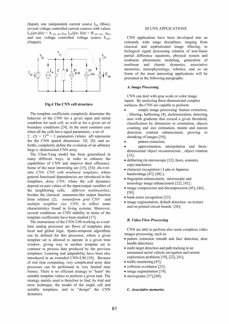
(Input), one independent current source Iijw (Bias), several voltage controlled current sources with values Ixy(ijw,klz) = A ijw, klz.yklz Ixu(ijw; klz) = B ijw; kl,z .uklz and one voltage controlled voltage source Eyijw (Output).

Fig.4 The CNN cell structure

The template coefficients completely determine the

behavior of the CNN for a given input and initial condition for each cell, as well as for a given set of boundary conditions [24]. In the most common case when all the cells have equal parameters, a set of 2 . (2r + 1)nD + 1 parameters (where nD represents the the CNN spatial dimension: 1D, 2D, and so-forth), completely define the evolution of an arbitrary large n -dimensional CNN array.

The Chua-Yang model has been generalized in many different ways, in order to enhance the capabilities of CNN and improve their efficiency. Some of the most interesting are [15], [54]: discrete-time CNN, CNN with nonlinear templates, where general functional dependencies are introduced in the templates, delay CNN, where the cell dynamics depend on past values of the input/output variables of the neighboring cells, different nonlinearities, besides the classical saturation-like output function from relation (2), nonuniform grid CNN and multiple neighbor size CNN, to reflect some characteristics found in living systems. Moreover, several conditions on CNN stability in terms of the template coefficients have been studied [17].

The instructions of the CNN-UM working as a real-time analog processor are flows of templates plus local and global logic. Spatio-temporal algorithms can be defined for this processor, where a given template set is allowed to operate in a given time window, giving way to another template set to continue to process data produced by the previous templates. Learning and adaptability have been also introduced in an extended CNN-UM [38]. Because of real time computing, very complicated array data processes can be performed in very limited time frames. There is no efficient strategy to "learn" the suitable template values to perform a given task. The strategy mainly used is therefore to find, by trial and error technique, the model of the single cell and suitable templates, and to "design" the CNN dynamics.

III CNN APPLICATIONS

CNN applications have been developed into an

extremely wide range disciplines, ranging from classical and sophisticated image filtering, to biological signal processing solution of non-linear partial difference equations, physical system and nonlinear phenomena modeling, generation of nonlinear and chaotic dynamics, associative memories, neurophysiology, robotics, and so on Some of the most interesting applications will be presented in the following paragraphs.

A. Image Processing

CNN can deal with gray-scale or color image inputs. By analyzing three-dimensional complex surfaces, the CNN are capable to perform: • simple image processing: feature extraction,

, filtering, halftoning [4], skeletonization, detecting area with gradients that exceed a given threshold, classification by dimension or orientation, objects counting and size estimation, minim and maxim detection, contrast enhancement, growing or shrinking of images [54];

• pattern extraction; • approximation, interpolation and three-

dimensional object reconstruction , object rotation [35];

• deblurring (in microscopic [32], faxes, scanners, copy-machines);

• character recognition ( Latin or Japanese handwritings [47], [48] );

• fingerprint enhancement, microscopic and neurology image enhancement [22], [42] ;

• image compression and decompression [45], [46], [50];

• bank-notes recognition [52]; • image segmentation, default detection on texture

and on printed circuit boards [26];

B. Video Flow Processing

CNN are able to perform also some complexe video images processing, such as: • pattern extraction (mouth and face detection, door

handle detection); • multi target detection and path tracking in an

unmanned aerial vehicle navigation and terrain exploration problems [19], [22], [41];

• traffic monitoring [47]; • collision avoidance [23]; • image segmentation [19]; • stereograms [37],[40];

C. Associative memories

61

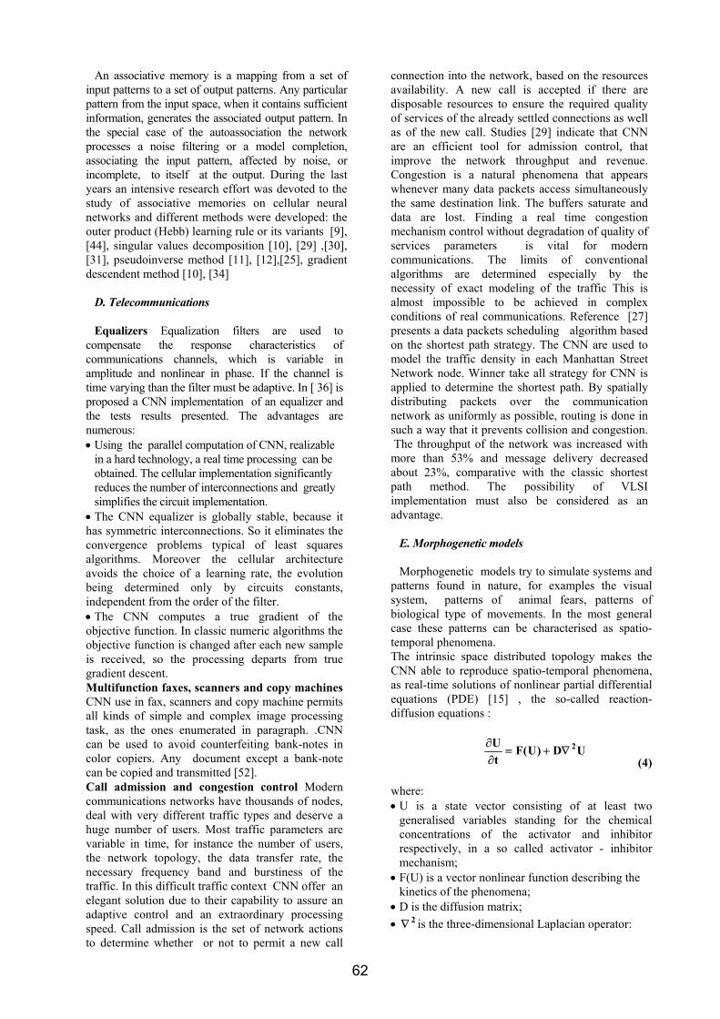
An associative memory is a mapping from a set of input patterns to a set of output patterns. Any particular pattern from the input space, when it contains sufficient information, generates the associated output pattern. In the special case of the autoassociation the network processes a noise filtering or a model completion, associating the input pattern, affected by noise, or incomplete, to itself at the output. During the last years an intensive research effort was devoted to the study of associative memories on cellular neural networks and different methods were developed: the outer product (Hebb) learning rule or its variants [9], [44], singular values decomposition [10], [29] ,[30], [31], pseudoinverse method [11], [12],[25], gradient descendent method [10], [34]

D. Telecommunications

Equalizers Equalization filters are used to compensate the response characteristics of communications channels, which is variable in amplitude and nonlinear in phase. If the channel is time varying than the filter must be adaptive. In [ 36] is proposed a CNN implementation of an equalizer and the tests results presented. The advantages are numerous: • Using the parallel computation of CNN, realizable

in a hard technology, a real time processing can be obtained. The cellular implementation significantly reduces the number of interconnections and greatly simplifies the circuit implementation.

• The CNN equalizer is globally stable, because it has symmetric interconnections. So it eliminates the convergence problems typical of least squares algorithms. Moreover the cellular architecture avoids the choice of a learning rate, the evolution being determined only by circuits constants, independent from the order of the filter. • The CNN computes a true gradient of the objective function. In classic numeric algorithms the objective function is changed after each new sample is received, so the processing departs from true gradient descent. Multifunction faxes, scanners and copy machines CNN use in fax, scanners and copy machine permits all kinds of simple and complex image processing task, as the ones enumerated in paragraph. .CNN can be used to avoid counterfeiting bank-notes in color copiers. Any document except a bank-note can be copied and transmitted [52]. Call admission and congestion control Modern communications networks have thousands of nodes, deal with very different traffic types and deserve a huge number of users. Most traffic parameters are variable in time, for instance the number of users, the network topology, the data transfer rate, the necessary frequency band and burstiness of the traffic. In this difficult traffic context CNN offer an elegant solution due to their capability to assure an adaptive control and an extraordinary processing speed. Call admission is the set of network actions to determine whether or not to permit a new call

connection into the network, based on the resources availability. A new call is accepted if there are disposable resources to ensure the required quality of services of the already settled connections as well as of the new call. Studies [29] indicate that CNN are an efficient tool for admission control, that improve the network throughput and revenue. Congestion is a natural phenomena that appears whenever many data packets access simultaneously the same destination link. The buffers saturate and data are lost. Finding a real time congestion mechanism control without degradation of quality of services parameters is vital for modern communications. The limits of conventional algorithms are determined especially by the necessity of exact modeling of the traffic This is almost impossible to be achieved in complex conditions of real communications. Reference [27] presents a data packets scheduling algorithm based on the shortest path strategy. The CNN are used to model the traffic density in each Manhattan Street Network node. Winner take all strategy for CNN is applied to determine the shortest path. By spatially distributing packets over the communication network as uniformly as possible, routing is done in such a way that it prevents collision and congestion. The throughput of the network was increased with more than 53% and message delivery decreased about 23%, comparative with the classic shortest path method. The possibility of VLSI implementation must also be considered as an advantage.

E. Morphogenetic models

Morphogenetic models try to simulate systems and patterns found in nature, for examples the visual system, patterns of animal fears, patterns of biological type of movements. In the most general case these patterns can be characterised as spatio-temporal phenomena. The intrinsic space distributed topology makes the CNN able to reproduce spatio-temporal phenomena, as real-time solutions of nonlinear partial differential equations (PDE) [15] , the so-called reaction-diffusion equations :

UD)U(FtU 2∇+=∂∂

(4)

where: • U is a state vector consisting of at least two

generalised variables standing for the chemical concentrations of the activator and inhibitor respectively, in a so called activator - inhibitor mechanism;

• F(U) is a vector nonlinear function describing the kinetics of the phenomena;

• D is the diffusion matrix; • 2∇ is the three-dimensional Laplacian operator:

62

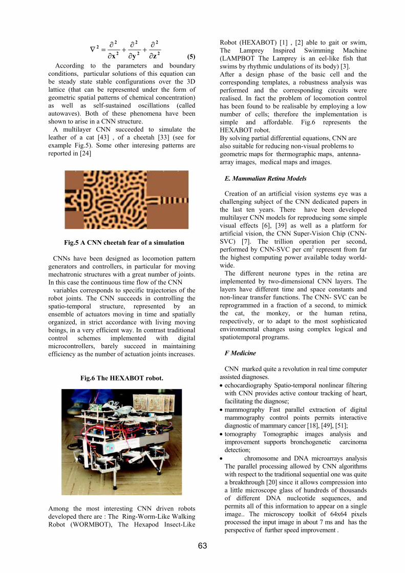
2

2

2

2

2

22

zyx ∂∂

+∂∂

+∂∂

=∇ (5)

According to the parameters and boundary

conditions, particular solutions of this equation can be steady state stable configurations over the 3D lattice (that can be represented under the form of geometric spatial patterns of chemical concentration) as well as self-sustained oscillations (called autowaves). Both of these phenomena have been shown to arise in a CNN structure.

A multilayer CNN succeeded to simulate the leather of a cat [43] , of a cheetah [33] (see for example Fig.5). Some other interesing patterns are reported in [24]

Fig.5 A CNN cheetah fear of a simulation

CNNs have been designed as locomotion pattern

generators and controllers, in particular for moving mechatronic structures with a great number of joints. In this case the continuous time flow of the CNN

variables corresponds to specific trajectories of the robot joints. The CNN succeeds in controlling the spatio-temporal structure, represented by an ensemble of actuators moving in time and spatially organized, in strict accordance with living moving beings, in a very efficient way. In contrast traditional control schemes implemented with digital microcontrollers, barely succeed in maintaining efficiency as the number of actuation joints increases.

Fig.6 The HEXABOT robot.

Among the most interesting CNN driven robots developed there are : The Ring-Worm-Like Walking Robot (WORMBOT), The Hexapod Insect-Like

Robot (HEXABOT) [1] , [2] able to gait or swim, The Lamprey Inspired Swimming Machine (LAMPBOT The Lamprey is an eel-like fish that swims by rhythmic undulations of its body) [3]. After a design phase of the basic cell and the corresponding templates, a robustness analysis was performed and the corresponding circuits were realised. In fact the problem of locomotion control has been found to be realisable by employing a low number of cells; therefore the implementation is simple and affordable. Fig.6 represents the HEXABOT robot. By solving partial differential equations, CNN are also suitable for reducing non-visual problems to geometric maps for thermographic maps, antenna-array images, medical maps and images.

E. Mammalian Retina Models

Creation of an artificial vision systems eye was a challenging subject of the CNN dedicated papers in the last ten years. There have been developed multilayer CNN models for reproducing some simple visual effects [6], [39] as well as a platform for artificial vision, the CNN Super-Vision Chip (CNN- SVC) [7]. The trillion operation per second, performed by CNN-SVC per cm2 represent from far the highest computing power available today world-wide.

The different neurone types in the retina are implemented by two-dimensional CNN layers. The layers have different time and space constants and non-linear transfer functions. The CNN- SVC can be reprogrammed in a fraction of a second, to mimick the cat, the monkey, or the human retina, respectively, or to adapt to the most sophisticated environmental changes using complex logical and spatiotemporal programs.

F Medicine

CNN marked quite a revolution in real time computer assisted diagnoses. • echocardiography Spatio-temporal nonlinear filtering

with CNN provides active contour tracking of heart, facilitating the diagnose;

• mammography Fast parallel extraction of digital mammography control points permits interactive diagnostic of mammary cancer [18], [49], [51];

• tomography Tomographic images analysis and improvement supports bronchogenetic carcinoma detection;

• chromosome and DNA microarrays analysis The parallel processing allowed by CNN algorithms with respect to the traditional sequential one was quite a breakthrough [20] since it allows compression into a little microscope glass of hundreds of thousands of different DNA nucleotide sequences, and permits all of this information to appear on a single image.. The microscopy toolkit of 64x64 pixels processed the input image in about 7 ms and has the perspective of further speed improvement .

63

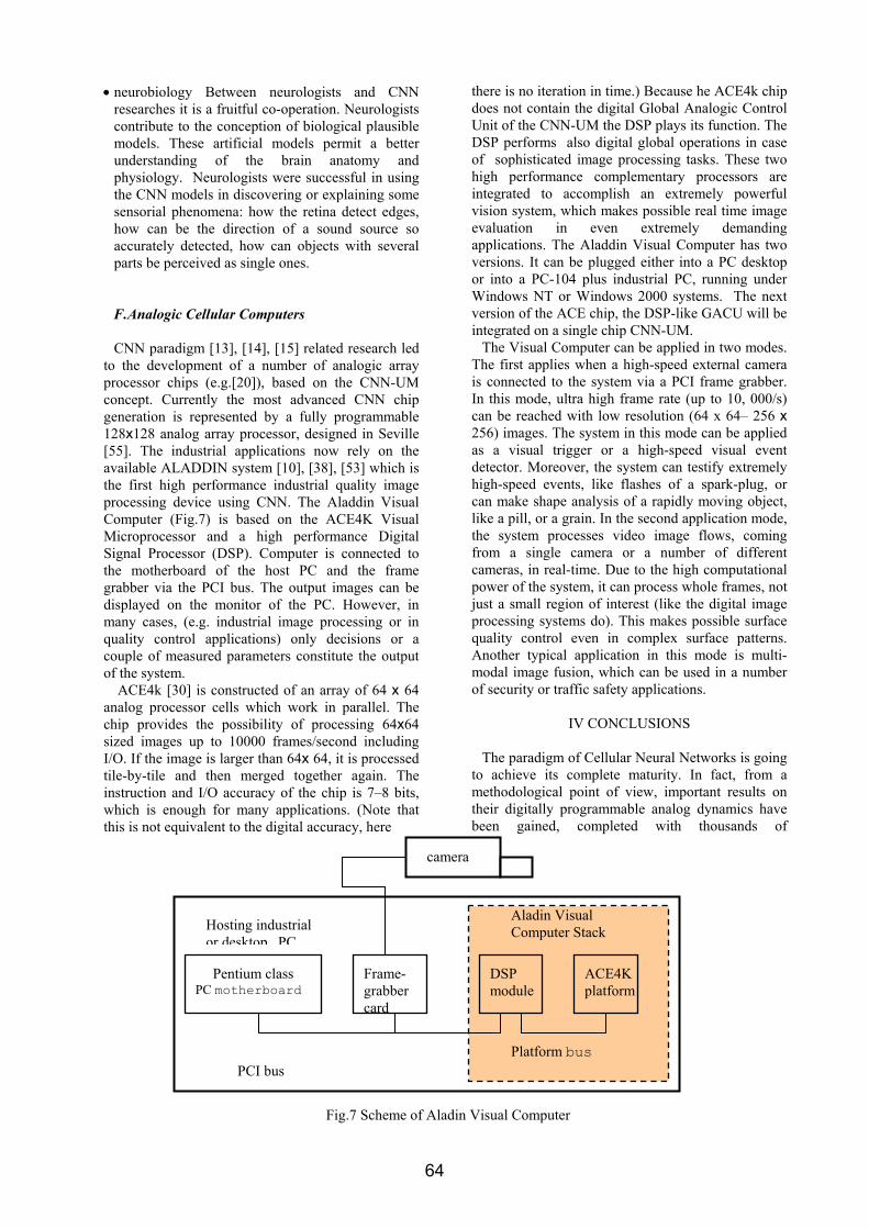
• neurobiology Between neurologists and CNN researches it is a fruitful co-operation. Neurologists contribute to the conception of biological plausible models. These artificial models permit a better understanding of the brain anatomy and physiology. Neurologists were successful in using the CNN models in discovering or explaining some sensorial phenomena: how the retina detect edges, how can be the direction of a sound source so accurately detected, how can objects with several parts be perceived as single ones.

F.Analogic Cellular Computers

CNN paradigm [13], [14], [15] related research led to the development of a number of analogic array processor chips (e.g.[20]), based on the CNN-UM concept. Currently the most advanced CNN chip generation is represented by a fully programmable 128x128 analog array processor, designed in Seville [55]. The industrial applications now rely on the available ALADDIN system [10], [38], [53] which is the first high performance industrial quality image processing device using CNN. The Aladdin Visual Computer (Fig.7) is based on the ACE4K Visual Microprocessor and a high performance Digital Signal Processor (DSP). Computer is connected to the motherboard of the host PC and the frame grabber via the PCI bus. The output images can be displayed on the monitor of the PC. However, in many cases, (e.g. industrial image processing or in quality control applications) only decisions or a couple of measured parameters constitute the output of the system.

ACE4k [30] is constructed of an array of 64 x 64 analog processor cells which work in parallel. The chip provides the possibility of processing 64x64 sized images up to 10000 frames/second including I/O. If the image is larger than 64x 64, it is processed tile-by-tile and then merged together again. The instruction and I/O accuracy of the chip is 7–8 bits, which is enough for many applications. (Note that this is not equivalent to the digital accuracy, here

there is no iteration in time.) Because he ACE4k chip does not contain the digital Global Analogic Control Unit of the CNN-UM the DSP plays its function. The DSP performs also digital global operations in case of sophisticated image processing tasks. These two high performance complementary processors are integrated to accomplish an extremely powerful vision system, which makes possible real time image evaluation in even extremely demanding applications. The Aladdin Visual Computer has two versions. It can be plugged either into a PC desktop or into a PC-104 plus industrial PC, running under Windows NT or Windows 2000 systems. The next version of the ACE chip, the DSP-like GACU will be integrated on a single chip CNN-UM.

The Visual Computer can be applied in two modes. The first applies when a high-speed external camera is connected to the system via a PCI frame grabber. In this mode, ultra high frame rate (up to 10, 000/s) can be reached with low resolution (64 x 64– 256 x 256) images. The system in this mode can be applied as a visual trigger or a high-speed visual event detector. Moreover, the system can testify extremely high-speed events, like flashes of a spark-plug, or can make shape analysis of a rapidly moving object, like a pill, or a grain. In the second application mode, the system processes video image flows, coming from a single camera or a number of different cameras, in real-time. Due to the high computational power of the system, it can process whole frames, not just a small region of interest (like the digital image processing systems do). This makes possible surface quality control even in complex surface patterns. Another typical application in this mode is multi-modal image fusion, which can be used in a number of security or traffic safety applications.

IV CONCLUSIONS

The paradigm of Cellular Neural Networks is going to achieve its complete maturity. In fact, from a methodological point of view, important results on their digitally programmable analog dynamics have been gained, completed with thousands of

Pentium class PC motherboard

Frame- grabber card

ACE4K platform

Aladin Visual Computer Stack

Platform bus PCI bus

Hosting industrial or desktop PC

DSP module

camera

Fig.7 Scheme of Aladin Visual Computer

64

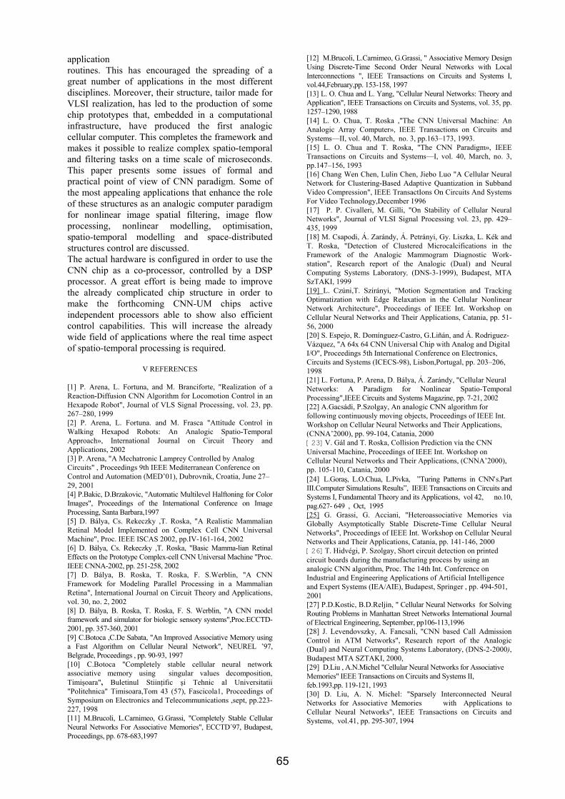
application routines. This has encouraged the spreading of a great number of applications in the most different disciplines. Moreover, their structure, tailor made for VLSI realization, has led to the production of some chip prototypes that, embedded in a computational infrastructure, have produced the first analogic cellular computer. This completes the framework and makes it possible to realize complex spatio-temporal and filtering tasks on a time scale of microseconds. This paper presents some issues of formal and practical point of view of CNN paradigm. Some of the most appealing applications that enhance the role of these structures as an analogic computer paradigm for nonlinear image spatial filtering, image flow processing, nonlinear modelling, optimisation, spatio-temporal modelling and space-distributed structures control are discussed. The actual hardware is configured in order to use the CNN chip as a co-processor, controlled by a DSP processor. A great effort is being made to improve the already complicated chip structure in order to make the forthcoming CNN-UM chips active independent processors able to show also efficient control capabilities. This will increase the already wide field of applications where the real time aspect of spatio-temporal processing is required.

V REFERENCES [1] P. Arena, L. Fortuna, and M. Branciforte, "Realization of a Reaction-Diffusion CNN Algorithm for Locomotion Control in an Hexapode Robot", Journal of VLS Signal Processing, vol. 23, pp. 267–280, 1999 [2] P. Arena, L. Fortuna. and M. Frasca "Attitude Control in Walking Hexapod Robots: An Analogic Spatio-Temporal Approach», International Journal on Circuit Theory and Applications, 2002 [3] P. Arena, "A Mechatronic Lamprey Controlled by Analog Circuits" , Proceedings 9th IEEE Mediterranean Conference on Control and Automation (MED’01), Dubrovnik, Croatia, June 27–29, 2001 [4] P.Bakic, D.Brzakovic, "Automatic Multilevel Halftoning for Color Images", Proceedings of the International Conference on Image Processing, Santa Barbara,1997 [5] D. Bálya, Cs. Rekeczky ,T. Roska, "A Realistic Mammalian Retinal Model Implemented on Complex Cell CNN Universal Machine", Proc. IEEE ISCAS 2002, pp.IV-161-164, 2002 [6] D. Bálya, Cs. Rekeczky ,T. Roska, "Basic Mamma-lian Retinal Effects on the Prototype Complex-cell CNN Universal Machine "Proc. IEEE CNNA-2002, pp. 251-258, 2002 [7] D. Bálya, B. Roska, T. Roska, F. S.Werblin, "A CNN Framework for Modeling Parallel Processing in a Mammalian Retina", International Journal on Circuit Theory and Applications, vol. 30, no. 2, 2002 [8] D. Bálya, B. Roska, T. Roska, F. S. Werblin, "A CNN model framework and simulator for biologic sensory systems",Proc.ECCTD-2001, pp. 357-360, 2001 [9] C.Botoca ,C.De Sabata, "An Improved Associative Memory using a Fast Algorithm on Cellular Neural Network", NEUREL ’97, Belgrade, Proceedings , pp. 90-93, 1997 [10] C.Botoca "Completely stable cellular neural network associative memory using singular values decomposition, Timişoara", Buletinul Stiinţific şi Tehnic al Universitatii "Politehnica" Timisoara,Tom 43 (57), Fascicola1, Proceedings of Symposium on Electronics and Telecommunications ,sept, pp.223-227, 1998 [11] M.Brucoli, L.Carnimeo, G.Grassi, "Completely Stable Cellular Neural Networks For Associative Memories", ECCTD´97, Budapest, Proceedings, pp. 678-683,1997

[12] M.Brucoli, L.Carnimeo, G.Grassi, " Associative Memory Design Using Discrete-Time Second Order Neural Networks with Local Interconnections ", IEEE Transactions on Circuits and Systems I, vol.44,February,pp. 153-158, 1997 [13] L. O. Chua and L. Yang, "Cellular Neural Networks: Theory and Application", IEEE Transactions on Circuits and Systems, vol. 35, pp. 1257–1290, 1988 [14] L. O. Chua, T. Roska ,"The CNN Universal Machine: An Analogic Array Computer», IEEE Transactions on Circuits and Systems—II, vol. 40, March, no. 3, pp.163–173, 1993. [15] L. O. Chua and T. Roska, "The CNN Paradigm», IEEE Transactions on Circuits and Systems—I, vol. 40, March, no. 3, pp.147–156, 1993 [16] Chang Wen Chen, Lulin Chen, Jiebo Luo "A Cellular Neural Network for Clustering-Based Adaptive Quantization in Subband Video Compression", IEEE TransactIons On Circuits And Systems For Video Technology,December 1996 [17] P. P. Civalleri, M. Gilli, "On Stability of Cellular Neural Networks", Journal of VLSI Signal Processing vol. 23, pp. 429–435, 1999 [18] M. Csapodi, Á. Zarándy, Á. Petrányi, Gy. Liszka, L. Kék and T. Roska, "Detection of Clustered Microcalcifications in the Framework of the Analogic Mammogram Diagnostic Work-station", Research report of the Analogic (Dual) and Neural Computing Systems Laboratory, (DNS-3-1999), Budapest, MTA SzTAKI, 1999 [19] L. Czúni,T. Szirányi, "Motion Segmentation and Tracking Optimatization with Edge Relaxation in the Cellular Nonlinear Network Architecture", Proceedings of IEEE Int. Workshop on Cellular Neural Networks and Their Applications, Catania, pp. 51-56, 2000 [20] S. Espejo, R. Domínguez-Castro, G.Liñán, and Á. Rodriguez-Vázquez, "A 64x 64 CNN Universal Chip with Analog and Digital I/O", Proceedings 5th International Conference on Electronics, Circuits and Systems (ICECS-98), Lisbon,Portugal, pp. 203–206, 1998 [21] L. Fortuna, P. Arena, D. Bálya, Á. Zarándy, "Cellular Neural Networks: A Paradigm for Nonlinear Spatio-Temporal Processing",IEEE Circuits and Systems Magazine, pp. 7-21, 2002 [22] A.Gacsádi, P.Szolgay, An analogic CNN algorithm for following continuously moving objects, Proceedings of IEEE Int. Workshop on Cellular Neural Networks and Their Applications, (CNNA’2000), pp. 99-104, Catania, 2000 [23]V. Gál and T. Roska, Collision Prediction via the CNN Universal Machine, Proceedings of IEEE Int. Workshop on Cellular Neural Networks and Their Applications, (CNNA’2000), pp. 105-110, Catania, 2000 [24] L.Goraş, L.O.Chua, L.Pivka, ”Turing Patterns in CNN′s.Part III.Computer Simulations Results”, IEEE Transactions on Circuits and Systems I, Fundamental Theory and its Applications, vol 42, no.10, pag.627- 649 , Oct, 1995 [25] G. Grassi, G. Acciani, "Heteroassociative Memories via Globally Asymptotically Stable Discrete-Time Cellular Neural Networks", Proceedings of IEEE Int. Workshop on Cellular Neural Networks and Their Applications, Catania, pp. 141-146, 2000 [26]T. Hidvégi, P. Szolgay, Short circuit detection on printed circuit boards during the manufacturing process by using an analogic CNN algorithm, Proc. The 14th Int. Conference on Industrial and Engineering Applications of Artificial Intelligence and Expert Systems (IEA/AIE), Budapest, Springer , pp. 494-501, 2001 [27] P.D.Kostic, B.D.Reljin, " Cellular Neural Networks for Solving Routing Problems in Manhattan Street Networks International Journal of Electrical Engineering, September, pp106-113,1996 [28] J. Levendovszky, A. Fancsali, "CNN based Call Admission Control in ATM Networks", Research report of the Analogic (Dual) and Neural Computing Systems Laboratory, (DNS-2-2000), Budapest MTA SZTAKI, 2000, [29] D.Liu , A.N.Michel "Cellular Neural Networks for Associative Memories" IEEE Transactions on Circuits and Systems II, feb.1993,pp. 119-121, 1993 [30] D. Liu, A. N. Michel: "Sparsely Interconnected Neural Networks for Associative Memories with Applications to Cellular Neural Networks", IEEE Transactions on Circuits and Systems, vol.41, pp. 295-307, 1994

65

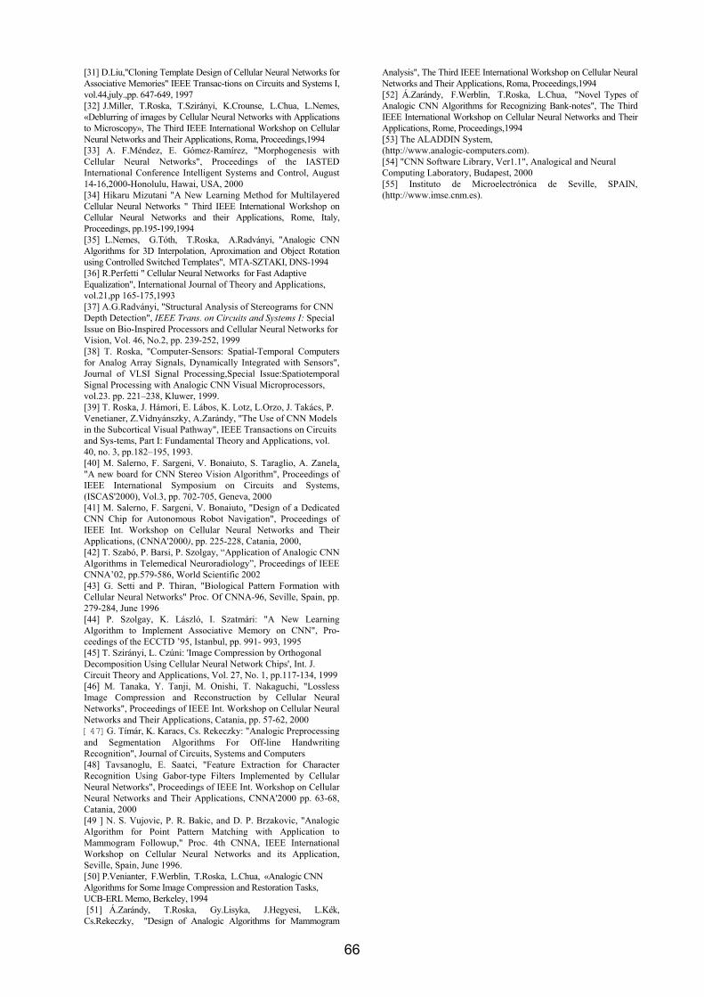
[31] D.Liu,"Cloning Template Design of Cellular Neural Networks for Associative Memories" IEEE Transac-tions on Circuits and Systems I, vol.44,july.,pp. 647-649, 1997 [32] J.Miller, T.Roska, T.Szirányi, K.Crounse, L.Chua, L.Nemes, «Deblurring of images by Cellular Neural Networks with Applications to Microscopy», The Third IEEE International Workshop on Cellular Neural Networks and Their Applications, Roma, Proceedings,1994 [33] A. F.Méndez, E. Gómez-Ramírez, "Morphogenesis with Cellular Neural Networks", Proceedings of the IASTED International Conference Intelligent Systems and Control, August 14-16,2000-Honolulu, Hawai, USA, 2000 [34] Hikaru Mizutani "A New Learning Method for Multilayered Cellular Neural Networks " Third IEEE International Workshop on Cellular Neural Networks and their Applications, Rome, Italy, Proceedings, pp.195-199,1994 [35] L.Nemes, G.Tóth, T.Roska, A.Radványi, "Analogic CNN Algorithms for 3D Interpolation, Aproximation and Object Rotation using Controlled Switched Templates", MTA-SZTAKI, DNS-1994 [36] R.Perfetti " Cellular Neural Networks for Fast Adaptive Equalization", International Journal of Theory and Applications, vol.21,pp 165-175,1993 [37] A.G.Radványi, "Structural Analysis of Stereograms for CNN Depth Detection", IEEE Trans. on Circuits and Systems I: Special Issue on Bio-Inspired Processors and Cellular Neural Networks for Vision, Vol. 46, No.2, pp. 239-252, 1999i [38] T. Roska, "Computer-Sensors: Spatial-Temporal Computers for Analog Array Signals, Dynamically Integrated with Sensors", Journal of VLSI Signal Processing,Special Issue:Spatiotemporal Signal Processing with Analogic CNN Visual Microprocessors, vol.23. pp. 221–238, Kluwer, 1999. [39] T. Roska, J. Hámori, E. Lábos, K. Lotz, L.Orzo, J. Takács, P. Venetianer, Z.Vidnyánszky, A.Zarándy, "The Use of CNN Models in the Subcortical Visual Pathway", IEEE Transactions on Circuits and Sys-tems, Part I: Fundamental Theory and Applications, vol. 40, no. 3, pp.182–195, 1993. [40] M. Salerno, F. Sargeni, V. Bonaiuto, S. Taraglio, A. Zanela, "A new board for CNN Stereo Vision Algorithm", Proceedings of IEEE International Symposium on Circuits and Systems, (ISCAS'2000), Vol.3, pp. 702-705, Geneva, 2000 [41] M. Salerno, F. Sargeni, V. Bonaiuto, "Design of a Dedicated CNN Chip for Autonomous Robot Navigation", Proceedings of IEEE Int. Workshop on Cellular Neural Networks and Their Applications, (CNNA'2000), pp. 225-228, Catania, 2000, [42] T. Szabó, P. Barsi, P. Szolgay, “Application of Analogic CNN Algorithms in Telemedical Neuroradiology”, Proceedings of IEEE CNNA’02, pp.579-586, World Scientific 2002 [43] G. Setti and P. Thiran, "Biological Pattern Formation with Cellular Neural Networks" Proc. Of CNNA-96, Seville, Spain, pp. 279-284, June 1996 [44] P. Szolgay, K. László, I. Szatmári: "A New Learning Algorithm to Implement Associative Memory on CNN", Pro-ceedings of the ECCTD ’95, Istanbul, pp. 991- 993, 1995 [45] T. Szirányi, L. Czúni: 'Image Compression by Orthogonal Decomposition Using Cellular Neural Network Chips', Int. J. Circuit Theory and Applications, Vol. 27, No. 1, pp.117-134, 1999 [46] M. Tanaka, Y. Tanji, M. Onishi, T. Nakaguchi, "Lossless Image Compression and Reconstruction by Cellular Neural Networks", Proceedings of IEEE Int. Workshop on Cellular Neural Networks and Their Applications, Catania, pp. 57-62, 2000 [47]G. Tímár, K. Karacs, Cs. Rekeczky: "Analogic Preprocessing and Segmentation Algorithms For Off-line Handwriting Recognition", Journal of Circuits, Systems and Computers [48] Tavsanoglu, E. Saatci, "Feature Extraction for Character Recognition Using Gabor-type Filters Implemented by Cellular Neural Networks", Proceedings of IEEE Int. Workshop on Cellular Neural Networks and Their Applications, CNNA'2000 pp. 63-68, Catania, 2000 [49 ] N. S. Vujovic, P. R. Bakic, and D. P. Brzakovic, "Analogic Algorithm for Point Pattern Matching with Application to Mammogram Followup," Proc. 4th CNNA, IEEE International Workshop on Cellular Neural Networks and its Application, Seville, Spain, June 1996. [50] P.Venianter, F.Werblin, T.Roska, L.Chua, «Analogic CNN Algorithms for Some Image Compression and Restoration Tasks, UCB-ERL Memo, Berkeley, 1994 [51] Á.Zarándy, T.Roska, Gy.Lisyka, J.Hegyesi, L.Kék, Cs.Rekeczky, "Design of Analogic Algorithms for Mammogram

Analysis", The Third IEEE International Workshop on Cellular Neural Networks and Their Applications, Roma, Proceedings,1994 [52] Á.Zarándy, F.Werblin, T.Roska, L.Chua, "Novel Types of Analogic CNN Algorithms for Recognizing Bank-notes", The Third IEEE International Workshop on Cellular Neural Networks and Their Applications, Rome, Proceedings,1994 [53] The ALADDIN System, (http://www.analogic-computers.com). [54] "CNN Software Library, Ver1.1", Analogical and Neural Computing Laboratory, Budapest, 2000 [55] Instituto de Microelectrónica de Seville, SPAIN, (http://www.imse.cnm.es).

66

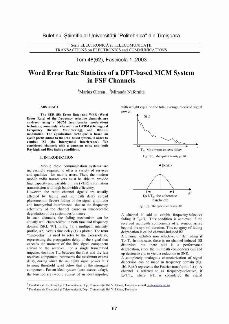
Buletinul Ştiinţific al Universităţii "Politehnica" din Timişoara

Seria ELECTRONICĂ şi TELECOMUNICAŢII TRANSACTIONS on ELECTRONICS and COMMUNICATIONS

Tom 48(62), Fascicola 1, 2003

Word Error Rate Statistics of a DFT-based MCM System

in FSF Channels

1Marius Oltean , 2Miranda Naforniţă

1 Facultatea de Electronică şi Teleomunicaţii, Dept. Comunicaţii, Bd. V. Pârvan, Timişoara, e-mail moltean@etc.utt.ro 2 Facultatea de Electronică şi Teleomunicaţii, Dept. Comunicaţii, Bd. V. Pârvan, Timişoara

ABSTRACT The BER (Bit Error Rate) and WER (Word Error Rate) of the frequency selective channels are analysed using a MCM (multicarrier modulation) technique, commonly referred to as OFDM (Orthogonal Frequency Division Multiplexing), and DBPSK modulation. The equalization technique is based on cyclic prefix added to the DFT based system, in order to combat ISI (the intersymbol interference). We considered channels with a gaussian noise and both Rayleigh and Rice fading conditions.

I. INTRODUCTION Mobile radio communication systems are increasingly required to offer a variety of services and qualities for mobile users. Then, the modern mobile radio transceivers must be able to provide high capacity and variable bit rate (VBR) information transmission with high bandwidth efficiency. However, the radio channel signals are usually affected by fading and multipath delay spread phenomenon. Severe fading of the signal amplitude and intersymbol interference due to the frequency selectivity of the channel cause an unacceptable degradation of the system performance. In such channels, the fading mechanism can be equally well characterized in both time and frequency domain [SKL ‘97]. In fig. 1a, a multipath intensity profile, s(τ), versus time delay (τ) is plotted. The term “time-delay” is used to refer to the excess-delay, representing the propagation delay of the signal that exceeds the moment of the first signal component arrival to the receiver. For a single transmitted impulse, the time Tm, between the first and the last received component, represents the maximum excess delay, during which the multipath signal power falls to some threshold level below that of the strongest component. For an ideal system (zero excess delay), the function s(τ) would consist of an ideal impulse,

with weight equal to the total average received signal power. A channel is said to exhibit frequency-selective fading if Tm>Ts. This condition is achieved if the received multipath components of a symbol arrive beyond the symbol duration. This category of fading degradation is called channel-induced ISI. A channel exhibits non selective, or flat fading if Tm<Ts. In this case, there is no channel-induced ISI distortion, but there still is a performance degradation, since the multipath components can add up destructively, to yield a reduction in SNR. A completely analogous characterization of signal dispersion can be made in frequency domain (fig. 1b). R(∆f) represents the Fourier transform of s(τ). A channel is referred to as frequency-selective, if f0<1/Ts, where 1/Ts is considered the signal

f0≈1/Tm, the coherence bandwidth

∆f

|R(∆f)|

Fig. 1(b). The coherence bandwidth

Fig. 1(a). Multipath intensity profile

Tm, Maximum excess delay τ

S(τ)

67

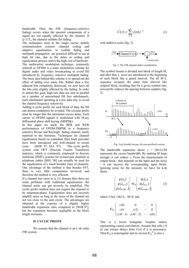
bandwidth. Thus, the FSF (frequency-selective fading) occurs when the spectral components of a signal are not equally affected by the channel. If f0>1/Ts, the channel exhibits flat fading. The techniques used in the single carrier mobile communication systems -channel coding and adaptive equalization- to combat fading and multipath propagation are practical difficult to use at high bit rate, due to the delay in coding and equalization process and to the high cost of hardware. The multicarrier modulation technique, commonly referred as OFDM is a main modulation scheme for digital audio and video broadcasting to avoid ISI introduced by frequency selective multipath fading. The basic idea behind this scheme is to spread-out the effect of fading over many bits. Rather then a few adjacent bits completely destroyed, we now have all the bits only slightly affected by the fading. In order to attend this goal, high-rate data are sent in parallel on a number of narrowband ISI free subchannels, each subchannel operating at a low data rate, to avoid the channel frequency selectivity. Adding a cyclic prefix for each block of data, the ISI can almost completely be avoided. The circular prefix must be longer that the maximum excess delay. Each carrier of OFDM signals is modulated with M-ary differential phase shift keying (MDPSK). In this paper we study the BER and WER performances of OFDM-DBPSK in a frequency selective Rician and Rayleigh fading channel, rarely reported in the literature. Techniques for channel equalization based on redundant filter bank precoder have been introduced and well-situated in recent years [SGB `97, XIA `97]. The cyclic prefix system with DFT (Discrete Fourier Transform) matrices, which is commonly employed in discrete multitone (DMT) systems for twisted pair channels in telephone cables [BIN `90] can actually be used for the equalization of a much broader class of channels. One advantage of the method is that besides FFT, there is very little computation involved, and therefore the method is very efficient. If a channel has zeros in |z |≥1 domain then there are some problems with traditional equalization: the channel noise can get severely be amplified. The cyclic prefix method does not require the channel to be minimum-phase. Equalization does not severely amplify noise as long as the zeros of the channel are not too close to the unit circle. The advantages are obtained at the expense of a slightly higher bandwidth expansion ratio compared to [SGB`97], but the expansion becomes negligible as the block length increases.

II. CYCLIC PREFIX

We assume that the channel is an L-th order

FIR system:

0

( ) ( )L

n

nC z c n z−

=

= ∑ (1)

with additive noise (fig. 2). The symbol stream is divided into block of length M, and after that, L zeros are introduced at the beginning of each block like a guard interval. The all M+L sequence occupies the same time interval like original block, resulting that for a given symbol rate, zero-prefix reduces the spacing between samples (fig. 3). The bandwidth expansion factor γ = (M+L)/M represents the excess bandwidth. By making M large enough, it can reduce γ. From the measurement of output block - that depends on the input and the noise - it can recover the corresponding input block. Ignoring noise for the moment, we have for k-th block:

⎥⎥⎥

⎦

⎤

⎢⎢⎢

⎣

⎡

−+

+

)()(

)(

1

1

Mk

k

k

JyJyJy

=C∆

⎥⎥⎥

⎦

⎤

⎢⎢⎢

⎣

⎡

−+

+

)()(

)(

1

1

Mk

k

k

JsJsJs

(2)

where J=k(L+M)+L, M>0, and

C∆=

⎟⎟⎟

⎠

⎞

⎜⎜⎜

⎝

⎛

−− )0()2()1(0)2()1(00)0(

cMcMccc

c

L

L

L

This is a lower triangular Toeplitz matrix representing causal convolution. Assume that c(0) ≠ 0 (it can extract delays from C(z) if it is necessary). Then C∆ is nonsingular and its inverse C∆

-1 is also a

a block of M symbols

a)

012

s (n)n

b))

0 LL zeros

x (n)

nL zeros

Fig. 3.(a) Symbol stream, (b) zero-prefixed version

Channel C(z) +s(n)

noise e(n)

Fig. 2. The FIR channel under consideration

y(n)

68

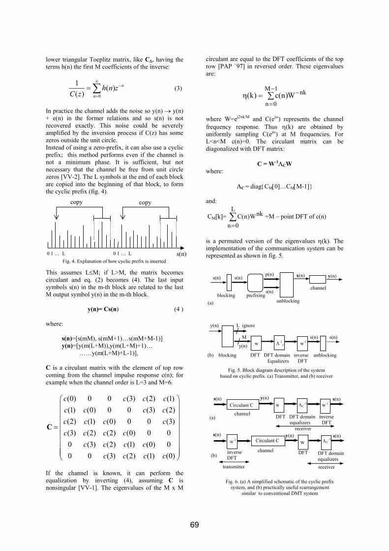
lower triangular Toeplitz matrix, like C∆, having the terms h(n) the first M coefficients of the inverse:

0

1 ( )( )

n

nh n z

C z

∞−

=

= ∑ (3)

In practice the channel adds the noise so y(n) → y(n) + e(n) in the former relations and so s(n) is not recovered exactly. This noise could be severely amplified by the inversion process if C(z) has some zeros outside the unit circle. Instead of using a zero-prefix, it can also use a cyclic prefix; this method performs even if the channel is not a minimum phase. It is sufficient, but not necessary that the channel be free from unit circle zeros [VV-2]. The L symbols at the end of each block are copied into the beginning of that block, to form the cyclic prefix (fig. 4). This assumes L≤M; if L>M, the matrix becomes circulant and eq. (2) becomes (4). The last input symbols s(n) in the m-th block are related to the last M output symbol y(n) in the m-th block.

y(n)= Cs(n) (4 )

where: s(n)=[s(mM), s(mM+1)…s(mM+M-1)] y(n)=[y(m(L+M)),y(m(L+M)+1)… ……y(m(L+M)+L-1)], C is a circulant matrix with the element of top row coming from the channel impulse response c(n); for example when the channel order is L=3 and M=6.

(0) 0 0 (3) (2) (1)(1) (0) 0 0 (3) (2)(2) (1) (0) 0 0 (3)(3) (2) (2) (0) 0 00 (3) (2) (1) (0) 00 0 (3) (2) (1) (0)

c c c cc c c cc c c cc c c c

c c c cc c c c

⎛ ⎞⎜ ⎟⎜ ⎟⎜ ⎟

= ⎜ ⎟⎜ ⎟⎜ ⎟⎜ ⎟⎜ ⎟⎝ ⎠

C

If the channel is known, it can perform the equalization by inverting (4), assuming C is nonsingular [VV-1]. The eigenvalues of the M x M

circulant are equal to the DFT coefficients of the top row [PAP `97] in reversed order. These eigenvalues are:

nk1M

0nW)n(c)k( −−

=∑=η

where W=ej2πk/M and C(ejω) represents the channel frequency response. Thus η(k) are obtained by uniformly sampling C(ejω) at M frequencies. For L<n<M c(n)=0. The circulant matrix can be diagonalized with DFT matrix:

C = W-1ΛCW where:

ΛC = diagCM[0]…CM[M-1] and:

CM[k]= ∑=

L

0n

nkW)n(C =M – point DFT of c(n)

is a permuted version of the eigenvalues η(k). The implementation of the communication system can be represented as shown in fig. 5.

y(n) L ignore M s(n) s(n) w Λ-1

c w-1

(b) blocking DFT DFT domain inverse unblocking Equalizers DFT

p(n) s(n)

blocking prefixing

s(n) x(n) y(n)

channel

unblocking (a)

Fig. 5. Block diagram description of the system based on cyclic prefix. (a) Transmitter, and (b) receiver

s(n)

y(n)

Fig. 6. (a) A simplified schematic of the cyclic prefix system, and (b) practically useful rearrangement

similar to conventional DMT system

s(n) y(n) s(n) Circulant C

channel

w ΛC-1 w-1

DFT DFT domain inverse equalizers DFT receiver

s(n)

(b)

(a)

channel

y(n) w-1 Circulant C w ΛC

-1

DFT DFT domain equalizers

inverse DFT

transmitter receiver

s(n)

0 1 … L 0 1 … L

copy copy

s(n) Fig. 4. Explanation of how cyclic prefix is inserted

69

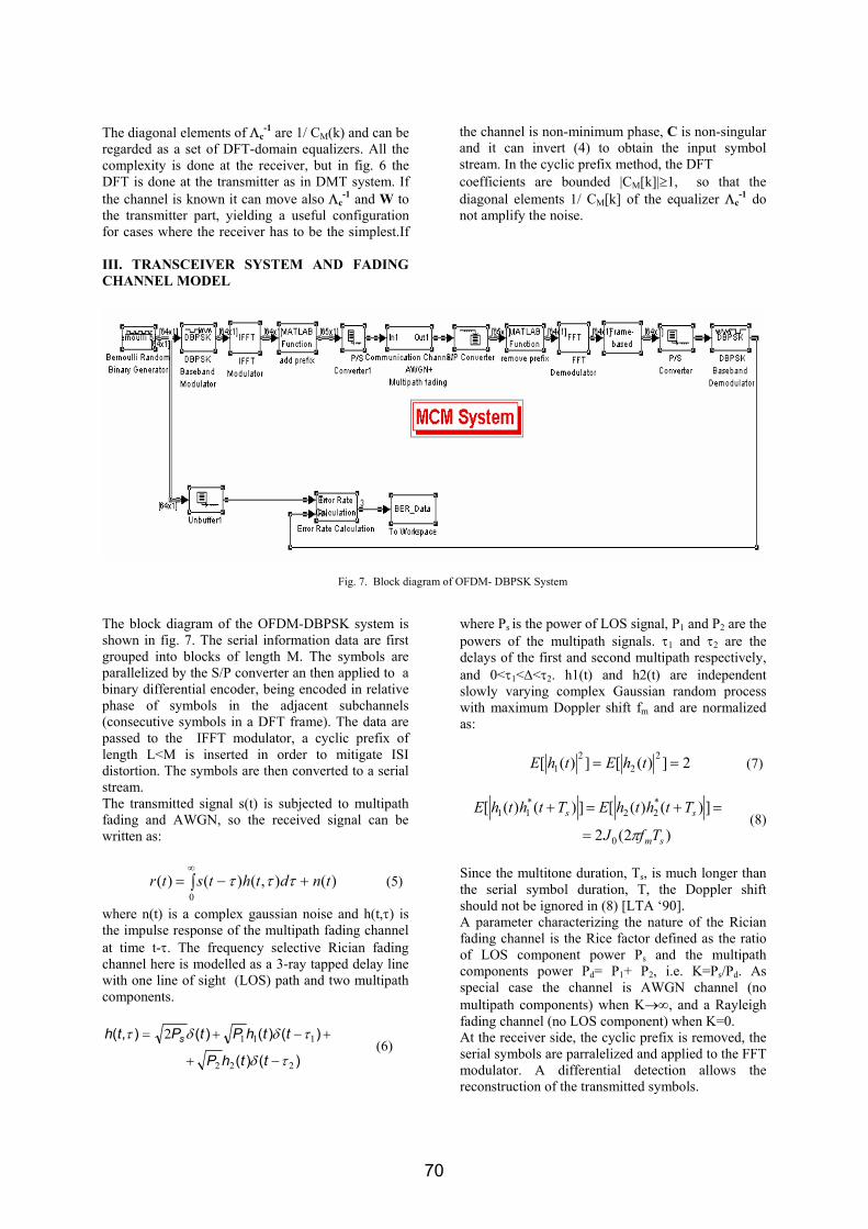
Fig. 7. Block diagram of OFDM- DBPSK System

The diagonal elements of Λc-1 are 1/ CM(k) and can be

regarded as a set of DFT-domain equalizers. All the complexity is done at the receiver, but in fig. 6 the DFT is done at the transmitter as in DMT system. If the channel is known it can move also Λc

-1 and W to the transmitter part, yielding a useful configuration for cases where the receiver has to be the simplest.If

the channel is non-minimum phase, C is non-singular and it can invert (4) to obtain the input symbol stream. In the cyclic prefix method, the DFT coefficients are bounded |CM[k]|≥1, so that the diagonal elements 1/ CM[k] of the equalizer Λc

-1 do not amplify the noise.

III. TRANSCEIVER SYSTEM AND FADING CHANNEL MODEL

The block diagram of the OFDM-DBPSK system is shown in fig. 7. The serial information data are first grouped into blocks of length M. The symbols are parallelized by the S/P converter an then applied to a binary differential encoder, being encoded in relative phase of symbols in the adjacent subchannels (consecutive symbols in a DFT frame). The data are passed to the IFFT modulator, a cyclic prefix of length L<M is inserted in order to mitigate ISI distortion. The symbols are then converted to a serial stream. The transmitted signal s(t) is subjected to multipath fading and AWGN, so the received signal can be written as:

∫∞

+−=0

)(),()()( tndthtstr τττ (5)

where n(t) is a complex gaussian noise and h(t,τ) is the impulse response of the multipath fading channel at time t-τ. The frequency selective Rician fading channel here is modelled as a 3-ray tapped delay line with one line of sight (LOS) path and two multipath components.

)()(

)()()(),(

222

1112

τδ

τδδτ

−+

+−+=

tthP

tthPtPth s (6)

where Ps is the power of LOS signal, P1 and P2 are the powers of the multipath signals. τ1 and τ2 are the delays of the first and second multipath respectively, and 0<τ1<∆<τ2. h1(t) and h2(t) are independent slowly varying complex Gaussian random process with maximum Doppler shift fm and are normalized as: 2])([])([ 2

22

1 == thEthE (7)

)2(2

])()([])()([

0

*22

*11

sm

ss

TfJ

TththETththE

π=

=+=+ (8)

Since the multitone duration, Ts, is much longer than the serial symbol duration, T, the Doppler shift should not be ignored in (8) [LTA ‘90]. A parameter characterizing the nature of the Rician fading channel is the Rice factor defined as the ratio of LOS component power Ps and the multipath components power Pd= P1+ P2, i.e. K=Ps/Pd. As special case the channel is AWGN channel (no multipath components) when K→∞, and a Rayleigh fading channel (no LOS component) when K=0. At the receiver side, the cyclic prefix is removed, the serial symbols are parralelized and applied to the FFT modulator. A differential detection allows the reconstruction of the transmitted symbols.

70

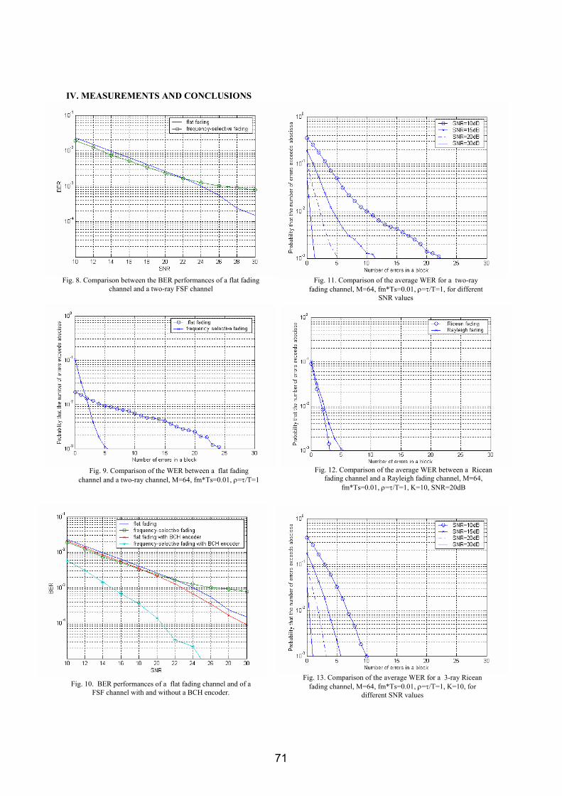
IV. MEASUREMENTS AND CONCLUSIONS

Fig. 9. Comparison of the WER between a flat fading channel and a two-ray channel, M=64, fm*Ts=0.01, ρ=τ/T=1

Fig. 11. Comparison of the average WER for a two-ray fading channel, M=64, fm*Ts=0.01, ρ=τ/T=1, for different

SNR values

Fig. 12. Comparison of the average WER between a Ricean fading channel and a Rayleigh fading channel, M=64,

fm*Ts=0.01, ρ=τ/T=1, K=10, SNR=20dB

Fig. 13. Comparison of the average WER for a 3-ray Ricean fading channel, M=64, fm*Ts=0.01, ρ=τ/T=1, K=10, for

different SNR values

Fig. 8. Comparison between the BER performances of a flat fading channel and a two-ray FSF channel

Fig. 10. BER performances of a flat fading channel and of a FSF channel with and without a BCH encoder.

71

From these simulations, it can be noticed that the BER of a 2-ray Rayleigh fading channel (we considered an equally amount of power for the two rays) is almost identical with that of a flat fading channel, until the values of SNR smaller than 22dB, when the BER becomes significantly better for the flat fading channel. Even if the BER of the two–ray channel is at best equal with the BER performances in a flat fading channel (fig.8) the average word error rate is better than that of a flat fading channel (fig.9). If a block code that can correct 6 errors in a block of 64 bits is employed, the frame error rate for the two-ray channel will be 10-3 , almost then times better than the frame error rate for a flat fading channel. Using this conclusion, we emphasized a significant BER performance improvement (fig.10) when a BCH encoder that can correct 10 errors in a block of 64 bits is used, (a coding gain up to 15 dB for the FSF channel). The price of this spectacular improvement is, of course, a two time higher transmission rate needed in order to transmit the same amount of data, due to the redundancy introduced by the BCH encoder. A comparison of the average WER for different SNR values was made (fig. 11). The illustrated result is a normal WER improvement if the average SNR increases. The WER performance of a 3-ray (Rice fading) channel is better than that of a 2-ray Rayleigh fading channel (fig. 12), as we would expect, due to the presence of the LOS component . In figure 13, we plotted the average WER for a 3-ray Ricean fading channel, considering different SNR values. The performance improves when SNR increases. At a certain SNR, the WER performance of the 3-ray Ricean fading channel is better than that of the 2-ray Rayleigh fading channel.

References: [SKL ‘97a] Sklar, B. , “Rayleigh fading channels in mobile digital communication systems ”, Part I, “Characterization”, IEEE Comm. Mag., July 1997. [SKL ‘97b] Sklar, B ., “Rayleigh fading channels in mobile digital communication systems ”, Part II, “Mitigation”, IEEE Comm. Mag., July 1997. [SGB ‘97a] Scaglione, A. , Giannakis, G.B.,and Barbarossa, S. “Redundant filter bank precoders and equalizers Part I: Unification and optimal designs” , IEEE Trans. Signal Processing, pp. 1988-2006, July 1999. [SGB ‘97b] Scaglione, A. , Giannakis, G.B.,and Barbarossa, S. “Redundant filter bank precoders and equalizers Part II: Synchronization and direct equalization”, IEEE Trans. Signal Processing, pp. 2007-2022, July 1999. [Xia ‘97] Xia, X-G, “New precoding for intersymbol interference cancellation using nonmaximally decimated multirate filter banks with ideal FIR equalizers”, IEEE Trans. Signal Processing, pp. 2431-2441, Oct. 1997. [BIN’ 90] Bingham, J. A. C. “Multicarrier modulation for data transmission: an idea whose time has come”, IEEE Comm. Mag., pp. 5-14, May 1990. [VV-1] Vrcely B. , Vaidyanathan P. P. “Pre - and post – processing for optimal noise reduction in cyclic prefix based channel equalizers”. [VV-2] Vrcely B. , Vaidyanathan P. P. “Fast and robust blind – equalization based on cyclic prefix”. [PAP’ 97] A. Papoulis, “Signal analysis”, McGraw Hill, 1997. [LTA ‘90] Lu, J. , Tjhung, T.T., Adachi, F. ,”BER performance of OFDM system in frequency-selective Rician fading with diversity reception”.

72

1,2“Politehnica” University of Timisoara, Communications Dept. For correspondence, please mail to corina@etc.utt.ro

Buletinul Ştiinţific al Universităţii "Politehnica" din Timişoara

Seria ELECTRONICĂ şi TELECOMUNICAŢII TRANSACTIONS on ELECTRONICS and COMMUNICATIONS

Tom 48(62), Fascicola 1, 2003

Digital Watermarking of Still Images using the Discrete Wavelet Transform

Corina Nafornita1, Alexandru Isar2 Abstract – We present a technique for the digital watermarking using a discrete wavelet transform. The proposed scheme is robust to a variety of signal distortions. When embedding the watermark, we make use of the image properties. To achieve imperceptibility, the lowest band of the image is left unmodified. To select the perceptually significant coefficients for each subband, we generate a watermarking key using an adaptive threshold. We compare our approach with another transform domain method. Simulation results show the robustness and validity of the watermarking process proposed herein. Keywords: copyright protection, digital watermarking, discrete wavelet transform.

I. INTRODUCTION Transmission, manipulation and storage of multimedia data are becoming an everyday practice. The rapid evolution of digital technology has led to the need of copyright protection tools [1]. One approach in this matter is cryptography. However, cryptography can protect content in transit, but once decrypted, the content has no further protection [2]. The alternative or complement to this approach is digital watermarking. Digital watermarking is the process of embedding information, called a watermark, in media signals, without making perceptible changes [3]. The watermark should be imperceptible, undeletable, statistically undetectable, robust to lossy compression and various signal distortions, and unambiguous [4]. Common types of signals to watermark are images, audio and video. In this paper, we concentrate on the application of digital watermarking of still images. Current techniques described in literature for the watermarking of images are spatial domain methods [8] and frequency domain methods [4, 5, 7, 9]. The spatial domain-watermarking scheme is generally fast and simple, but it doesn’t guarantee robustness against common signal distortions, like JPEG compression or noise. In this paper, we propose a frequency domain method, based on a multiresolution wavelet decomposition, which shows greater robustness against such common attacks.

This paper is organized as follows. In Section II, we introduce the proposed method for the digital watermarking. In Section III, we present the simulations results, and in Section IV, we provide some concluding remarks.

II. THE PROPOSED WATERMARKING TECHNIQUE

In this section, we explain the chosen method for embedding the watermark. Enhancing the perceptual invisibility hinges on considering the characteristics of the original image, e.g. modifications of high frequencies or of the high luminance regions are less perceptible. Similar to the human eye, the discrete wavelet transform decomposes an image in subbands having a bandwidth approximately equal on a logarithmic scale. Therefore, it is probable that small changes in some of the coefficients localized in the subbands that represent the detail images will make the mark imperceptible to human eyes. To achieve imperceptibility, the lowest band of the image is left unmodified. To select the perceptually significant coefficients for each subband, we generate a watermarking key using an adaptive threshold. We present two versions of the same watermarking method. A. Architecture We assume that the binary watermark is of length wN ,

and consists of elements from the set 1,1− . Let OI be the original image. We embed the watermark into the detail wavelet coefficients using a watermarking key, only in the first level of the decomposed image. The following steps are to be performed:

1. Compute the first level wavelet decomposition of the original image. We obtain one approximation image and three detail images, corresponding to the horizontal, vertical and diagonal details of the image. We denote the

73

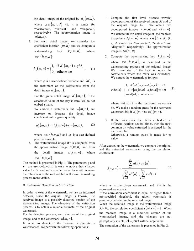
xth detail image of the original by ( )nmd x , ,

where dvhx ,,∈ (h, v, d stands for “horizontal”, “vertical” and “diagonal”, respectively). The approximation image is

),( nma . 2. For each detail image, we consider the

coefficient location ( )nm, and we compute a

watermarking key ( )nmkx , , where

dvhx ,,∈ :

( ) ( ) >

= otherwise ,0

, if ,1, xx

x

qMnmdnmk ,

(1)

where q is a user-defined variable and xM is the maximum of the coefficients from the detail image ( )nmd x , .

For the given detail image ( )nmd x , , if the associated value of the key is zero, we do not embed a mark. To embed a watermark bit ( )nmw , , we increase or decrease the detail image coefficient with a given quantity:

( ) ( ) ( )nmwnmdnmd xx ,,, α+=′ , (2)

where dvhx ,,∈ and α is a user-defined positive variable.

3. The watermarked image WI is computed from the approximation image ),( nma and from

the detail images ),( nmd x′ , where

dvhx ,,∈ . The method is presented in Fig.1. The parameters q and α are user-defined. It is easy to notice that a larger value for α and and a smaller value for q will increase the robustness of the method, but will make the marking process more visible. B. Watermark Detection and Extraction In order to extract the watermark, we use an informed detector, since the original image is known. The received image is a possibly distorted version of the watermarked image. The objective of the extraction process is to obtain a reliable estimate of the original watermark. For the detection process, we make use of the original image, and of the watermark ( )nmw , . In order to detect if the received image RI is watermarked, we perform the following operations:

1. Compute the first level discrete wavelet decomposition of the received image RI and of the original image OI. We obtain two decomposed images ),( nmr and ),( nmo . We denote the xth detail image of the received image by ( )nmrd x , , where dvhx ,,∈ (h, v, d stands for “horizontal”, “vertical” and “diagonal”, respectively). The approximation image is ),( nmra .

2. Compute the watermarking key ( )nmkx , ,

where dvhx ,,∈ , as described in the watermarking process of the original image. We make use of the key to locate the coefficients where the mark was embedded. We extract the watermark as follows:

( )( ) ( )[ ]( ) ( )[ ]

−<−−>−

= otherwise ),1,1(

0/,, if ,10/,, if ,1

,rand

nmdnmrdnmdnmrd

nmrw xx

xx

αα

(3)

where ( )nmrw , is the recovered watermark bit. We make a random guess for the recovered watermark bit, if ( ) ( )nmrdnmd xx ,, = .

3. If the watermark had been embedded in

different locations several times, then the most common bit value extracted is assigned for the recovered bit. Otherwise, a random guess is made for its value.

After extracting the watermark, we compare the original and the extracted watermarks using the correlation coefficient:

( )( ) ( )

( ) ( )∑∑

∑

==

=

⋅

⋅=

ww

w

N

n

N

n

N

n

nrwnw

nrwnwrwwc

1

2

1

2

1, ,

(4)

where w is the given watermark, and rw is the recovered watermark. If the correlation coefficient is equal or higher than a pre-specified threshold, the given watermark is positively detected in the received image. When the received image is the watermarked image RI=WI, the correlation coefficient ( ) .1, =rwwc When the received image is a modified version of the watermarked image, and the changes are not perceptually visible, ( )rwwc , will be large value. The extraction of the watermark is presented in Fig. 2.

74

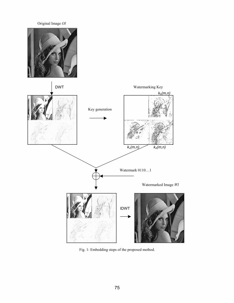
Fig. 1: Embedding steps of the proposed method.

DWT

Original Image OI

Key generation

Watermark 0110…1

kv(m,n) kd(m,n)

kh(m,n) Watermarking Key

IDWT

Watermarked Image WI

75

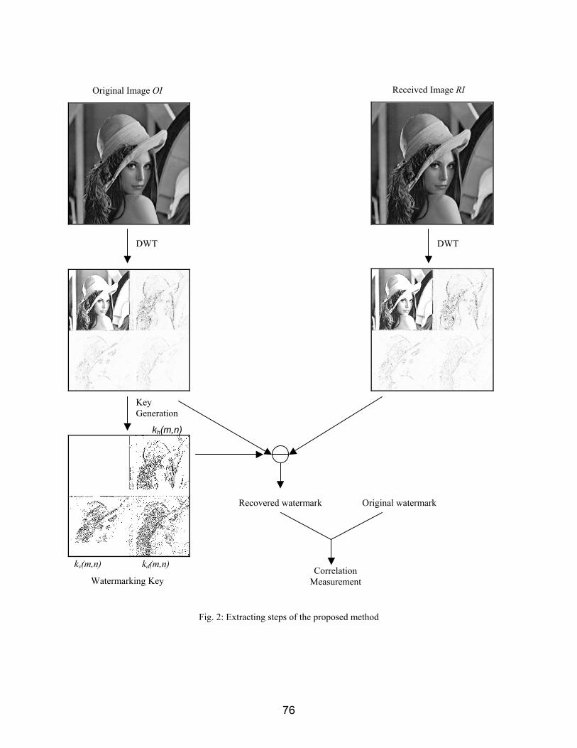
Fig. 2: Extracting steps of the proposed method

Original Image OI

DWT

Key Generation

kh(m,n)

kd(m,n) kv(m,n)

Watermarking Key

DWT

Recovered watermark Original watermark

Correlation Measurement

Received Image RI

76

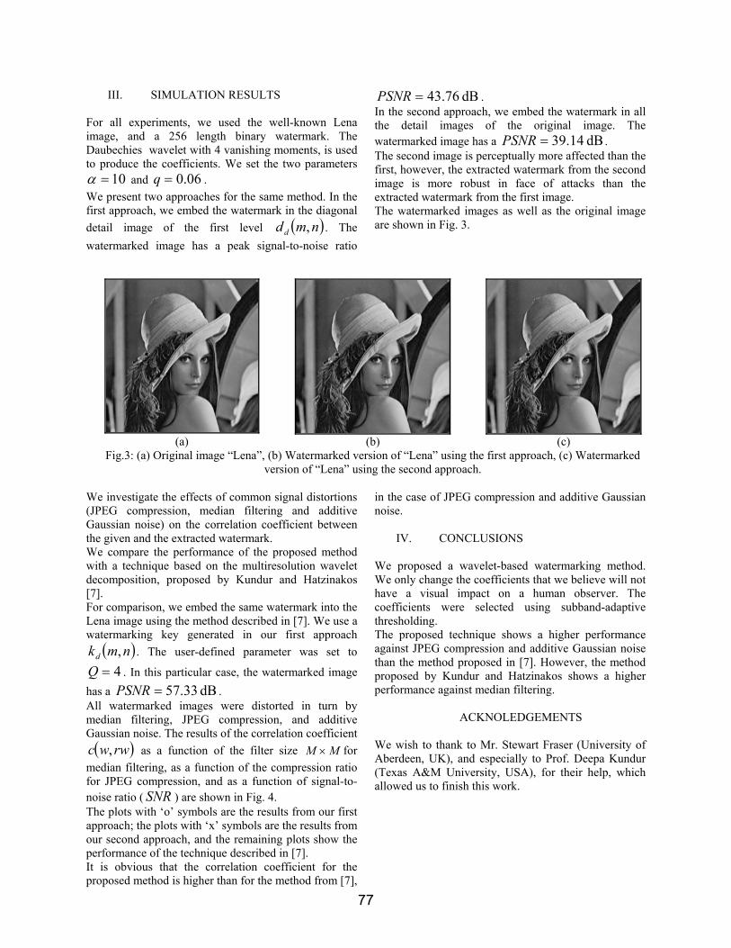
III. SIMULATION RESULTS For all experiments, we used the well-known Lena image, and a 256 length binary watermark. The Daubechies wavelet with 4 vanishing moments, is used to produce the coefficients. We set the two parameters

10=α and 06.0=q . We present two approaches for the same method. In the first approach, we embed the watermark in the diagonal detail image of the first level ( )nmdd , . The watermarked image has a peak signal-to-noise ratio

dB 76.43=PSNR . In the second approach, we embed the watermark in all the detail images of the original image. The watermarked image has a dB 14.39=PSNR . The second image is perceptually more affected than the first, however, the extracted watermark from the second image is more robust in face of attacks than the extracted watermark from the first image. The watermarked images as well as the original image are shown in Fig. 3.

We investigate the effects of common signal distortions (JPEG compression, median filtering and additive Gaussian noise) on the correlation coefficient between the given and the extracted watermark. We compare the performance of the proposed method with a technique based on the multiresolution wavelet decomposition, proposed by Kundur and Hatzinakos [7]. For comparison, we embed the same watermark into the Lena image using the method described in [7]. We use a watermarking key generated in our first approach

( )nmkd , . The user-defined parameter was set to

4=Q . In this particular case, the watermarked image has a dB 33.57=PSNR . All watermarked images were distorted in turn by median filtering, JPEG compression, and additive Gaussian noise. The results of the correlation coefficient ( )rwwc , as a function of the filter size MM × for

median filtering, as a function of the compression ratio for JPEG compression, and as a function of signal-to-noise ratio ( SNR ) are shown in Fig. 4. The plots with ‘o’ symbols are the results from our first approach; the plots with ‘x’ symbols are the results from our second approach, and the remaining plots show the performance of the technique described in [7]. It is obvious that the correlation coefficient for the proposed method is higher than for the method from [7],

in the case of JPEG compression and additive Gaussian noise.

IV. CONCLUSIONS

We proposed a wavelet-based watermarking method. We only change the coefficients that we believe will not have a visual impact on a human observer. The coefficients were selected using subband-adaptive thresholding. The proposed technique shows a higher performance against JPEG compression and additive Gaussian noise than the method proposed in [7]. However, the method proposed by Kundur and Hatzinakos shows a higher performance against median filtering.

ACKNOLEDGEMENTS We wish to thank to Mr. Stewart Fraser (University of Aberdeen, UK), and especially to Prof. Deepa Kundur (Texas A&M University, USA), for their help, which allowed us to finish this work.

(a) (b) (c)

Fig.3: (a) Original image “Lena”, (b) Watermarked version of “Lena” using the first approach, (c) Watermarked version of “Lena” using the second approach.

77

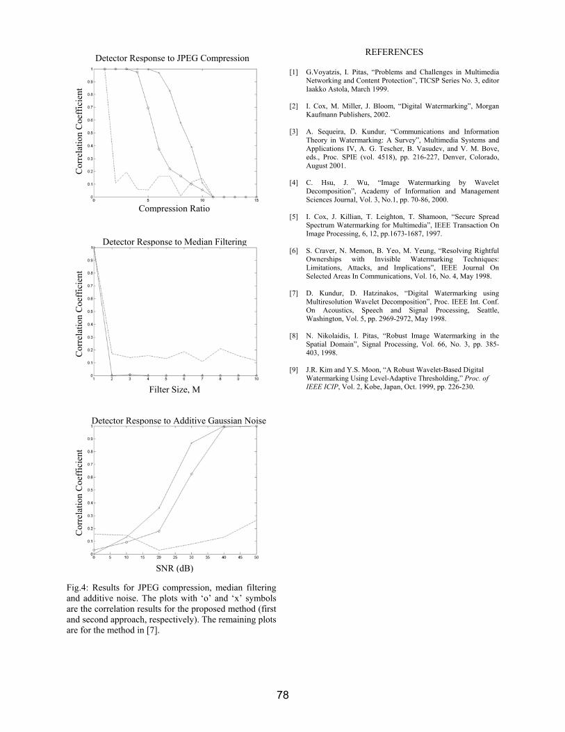
Fig.4: Results for JPEG compression, median filtering and additive noise. The plots with ‘o’ and ‘x’ symbols are the correlation results for the proposed method (first and second approach, respectively). The remaining plots are for the method in [7].

REFERENCES

[1] G.Voyatzis, I. Pitas, “Problems and Challenges in Multimedia Networking and Content Protection”, TICSP Series No. 3, editor Iaakko Astola, March 1999.

[2] I. Cox, M. Miller, J. Bloom, “Digital Watermarking”, Morgan

Kaufmann Publishers, 2002. [3] A. Sequeira, D. Kundur, “Communications and Information

Theory in Watermarking: A Survey”, Multimedia Systems and Applications IV, A. G. Tescher, B. Vasudev, and V. M. Bove, eds., Proc. SPIE (vol. 4518), pp. 216-227, Denver, Colorado, August 2001.

[4] C. Hsu, J. Wu, “Image Watermarking by Wavelet

Decomposition”, Academy of Information and Management Sciences Journal, Vol. 3, No.1, pp. 70-86, 2000.

[5] I. Cox, J. Killian, T. Leighton, T. Shamoon, “Secure Spread

Spectrum Watermarking for Multimedia”, IEEE Transaction On Image Processing, 6, 12, pp.1673-1687, 1997.

[6] S. Craver, N. Memon, B. Yeo, M. Yeung, “Resolving Rightful

Ownerships with Invisible Watermarking Techniques: Limitations, Attacks, and Implications”, IEEE Journal On Selected Areas In Communications, Vol. 16, No. 4, May 1998.

[7] D. Kundur, D. Hatzinakos, “Digital Watermarking using

Multiresolution Wavelet Decomposition”, Proc. IEEE Int. Conf. On Acoustics, Speech and Signal Processing, Seattle, Washington, Vol. 5, pp. 2969-2972, May 1998.

[8] N. Nikolaidis, I. Pitas, “Robust Image Watermarking in the

Spatial Domain”, Signal Processing, Vol. 66, No. 3, pp. 385-403, 1998.

[9] J.R. Kim and Y.S. Moon, “A Robust Wavelet-Based Digital

Watermarking Using Level-Adaptive Thresholding,” Proc. of IEEE ICIP, Vol. 2, Kobe, Japan, Oct. 1999, pp. 226-230.

Cor

rela

tion

Coe

ffic

ient

Detector Response to JPEG Compression

Detector Response to Median Filtering

Cor

rela

tion

Coe

ffic

ient

Filter Size, M

SNR (dB)

Cor

rela

tion

Coe

ffic

ient

Detector Response to Additive Gaussian Noise

Compression Ratio

78

1,2 „Politehnica” University of Timişoara, Faculty of Electronics and Telecommunications Bd. V. Pârvan No.2 e-mail salagean@etc.utt.ro 3 University of Oradea, Faculty of Electrotechnics and Informatics, , e-mail cgordan@uoradea.ro

Buletinul Ştiinţific al Universităţii "Politehnica" din Timişoara

Seria ELECTRONICĂ şi TELECOMUNICAŢII TRANSACTIONS on ELECTRONICS and COMMUNICATIONS

Tom 48(62), Fascicola 1, 2003

Instantaneous Frequency and its Determination

Marius Sălăgean1, Mirela Bianu2, Cornelia Gordan3

Abstract This paper presents the instantaneous frequency, the most important techniques in instantaneous frequency determination for nonstationary signals and some representatives’ simulations. Key words: instantaneous frequency (IF), Wigner-Ville distribution, multicomponent signals. I. INTRODUCTION The instantaneous frequency of a signal is a parameter used in communications, seismic processing, radar signals and biomedical applications. The IF is a good descriptor of some physical phenomenon. The importance of the instantaneous frequency result from the fact that in many applications the signals is often nonstationary, a simple example being the chirp signal. In seismic processing these signals have the advantage that their spectral characteristics can be controlled including duration, bandwidth and energy. Another application is for estimation of Doppler frequency shift in radar returns. For all these signals, the IF is an important characteristic. II. FREQUENCY ESTIMATION TECHNIQUES The signal model which has often used is: ( ) ( )2j fnz n Ae nπ ε= +

where A is the amplitude, f is the frequency,

( )z n is the discrete complex observation sequence

and ( )nε is the complex white Gaussian noise sequence [1]. The estimate for the frequency of a single sinusoid in white Gaussian noise has been shown to be given by finding that frequency at which the spectrum attains its maximum. This may be implemented with an initial coarse search on the bins of a Fast Fourier Transform (FFT) and a subsequent interpolation procedure. As long as the coarse frequency estimate falls within the main lobe of the frequency response, this technique converges to the correct global maximum. This estimate meets the Cramer-Rao bound (CRB) above a SNR threshold, the bound being given by:

( ) ( ) ( )2 2 2 2

12ˆ2 / 1

disp fA N Nπ σ

⎡ ⎤ ≥⎣ ⎦ −

where N is the number of independent samples in data, A is the signal amplitude and 22σ is the complex noise variance. The estimated variance departs quite dramatically from the CR bound once the SNR falls below a threshold value, a phenomenom that is common in nonlinear estimators. This method can be computationally too intensive in some applications. In an attempt to find frequency estimators, which reduce computation, many researchers have turned to parametric methods. These methods model the signal as having a rational transfer function. It is often computationally advantageous to assume that the numerator of the transfer function is a constant. Such models are said to be auto-regressive (AR), or linear predictive. Tretter introduced another frequency estimation technique [8]. He showed that for a complex sinusoid in white Gaussian noise at high SNR, the phase might be approximated well as a linear function of time, imbedded in an additive white Gaussian noise process. He used a linear regression technique to estimate the frequency. One problem with Tretter’s algorithm is that the first stage of the algorithm necessitates extracting the phase from data. This can be the source to significant errors. Kay obtained a modified form of this estimator by fitting a model to adjacent phase difference estimates, rather than the phase values themselves, thus avoiding the phase unwrapping problem. The resulting estimator is simply a smoothing of phase differences with a quadric window. The methods described in this section have dealt specifically with sinusoidal frequency estimation. They provide a good basis to understand the more complicated problem of estimating time-varying frequencies.

79

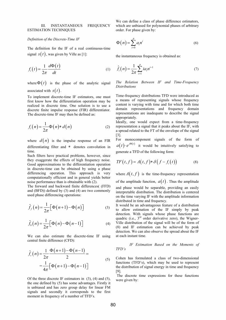
III. INSTANTANEOUS FREQUENCY ESTIMATION TECHNIQUES Definition of the Discrete-Time IF The definition for the IF of a real continuous-time signal ( )s t , was given by Ville as [1]:

( ) ( )12i

d tf t

dtπΦ

= (1)

where ( )tΦ is the phase of the analytic signal

associated with ( )s t . To implement discrete-time IF estimators, one must first know how the differentiation operation may be realized in discrete time. One solution is to use a discrete finite impulse response (FIR) differentiator. The discrete-time IF may then be defined as:

( ) ( ) ( )12if n n d nπ

= Φ ∗ (2)

where ( )d n is the impulse response of an FIR differentiating filter and ∗ denotes convolution in time. Such filters have practical problems, however, since they exaggerate the effects of high frequency noise. Good approximations to the differentiation operation in discrete-time can be obtained by using a phase differencing operation. This approach is very computationally efficient and in general yields better noise performance than is obtainable with (2). The forward and backward finite differences( (FFD) and (BFD)) defined by (3) and (4) are two commonly used phase differencing operations:

( ) ( ) ( )1ˆ 12ff n n nπ

= Φ + −Φ⎡ ⎤⎣ ⎦ (3)

( ) ( ) ( )1ˆ 12bf n n nπ

= Φ −Φ −⎡ ⎤⎣ ⎦ (4)

We can also estimate the discrete-time IF using central finite difference (CFD):

( ) ( ) ( )

( ) ( )

1 11ˆ2 21 = 1 1

4

c

n nf n

n n

π

π

Φ + −Φ −= =

Φ + −Φ −⎡ ⎤⎣ ⎦

(5)

Of the three discrete IF estimators in (3), (4) and (5), the one defined by (5) has some advantages. Firstly it is unbiased and has zero group delay for linear FM signals and secondly it corresponds to the first moment in frequency of a number of TFD’s.

We can define a class of phase difference estimators, which are unbiased for polynomial phases of arbitrary order. For phase given by:

( )0

pi

ii

n a n=

Φ =∑ (6)

the instantaneous frequency is obtained as:

( ) 1

1

1ˆ2

pi

i ii

f n ia nπ

−

=

= ∑ (7)

The Relation Between IF and Time-Frequency Distributions Time-frequency distributions TFD were introduced as a means of representing signals whose frequency content is varying with time and for which both time domain representations and frequency domain representations are inadequate to describe the signal appropriately. Ideally, one would expect from a time-frequency representation a signal that it peaks about the IF, with a spread related to the FT of the envelope of the signal [3]. For monocomponent signals of the form of

( ) ( )j ta t e Φ⋅ it would be intuitively satisfying to generate a TFD of the following form:

( ) ( ) ( )( ), , iTF t f A t f f f tδ= ∗ − (8) where ( ),A t f is the time-frequency representation

of the amplitude function, ( )a t . Thus the amplitude and phase would be separable, providing an easily interpretable distribution. The distribution is centered on the time varying IF with the amplitude information distributed in time and frequency. It would be an advantageous feature of a distribution to allow estimation of the IF simply by peak detection. With signals whose phase functions are quadric (i.e., 3rd order derivative zero), the Wigner-Ville distribution of the signal will be of the form of (8) and IF estimation can be achieved by peak detection. We can also observe the spread about the IF at each instant time.

IF Estimation Based on the Moments of

TFD’s Cohen has formulated a class of two-dimensional functions (TFD’s), which may be used to represent the distribution of signal energy in time and frequency [9]. The discrete time expressions for these functions were given by:

80

( ) ( ) ( )

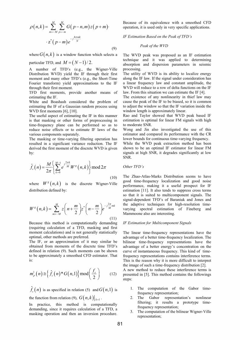
( )4

*

, ,

z

M M

m M p m

mkjN

n k G p n m z p m

p m eπ

ρ=− =−

−

= − + ⋅

⋅ −

∑ ∑

(9) where ( ),G n k is a window function which selects a

particular TFD, and ( )1 / 2.M N= − A number of TFD’s (e.g., the Wigner-Ville Distribution WVD) yield the IF through their first moment and many other TFD’s (e.g., the Short-Time Fourier transform) yield approximations to the IF through their first moment. TFD first moments, provide another means of estimating the IF. White and Boashash considered the problem of estimating the IF of a Gaussian random process using WVD first moments [6], [10]. The useful aspect of estimating the IF in this manner is that masking or other forms of preprocessing in time-frequency plane can be performed so as to reduce noise effects or to estimate IF laws of the various components separately. The masking or time-varying filtering operation has resulted in a significant variance reduction. The IF derived the first moment of the discrete WVD is given by:

( ) ( )21

0

ˆ , mod 22

kM j gMc

k

Mf n e W n kπ

ππ

−

=

⎧ ⎫= ⎨ ⎬

⎩ ⎭∑

(10) where ( ),gW n k is the discrete Wigner-Ville distribution defined by:

( )2

*,2 2

M j mkg M

m M

m mW n k z n z n eπ

−

=−

⎛ ⎞ ⎛ ⎞= + −⎜ ⎟ ⎜ ⎟⎝ ⎠ ⎝ ⎠

∑

(11) Because this method is computationally demanding (requiring calculation of a TFD, masking and first moment calculations) and is not generally statistically optimal, other methods are preferred. The IF, or an approximation of it may similar be obtained from moments of the discrete time TFD’s defined in relation (9). Such moments can be shown to be approximately a smoothed CFD estimator. That is:

( ) ( ) ( ) 1 ˆ * ,1 mod2

sc

fm n f n G nρ⎛ ⎞≅ ⎜ ⎟⎝ ⎠

(12)

( )cf n is as specified in relation (5) and ( ),1G n is

the function from relation (9), ( ) 1, kG n k = . In practice, this method is computationally demanding, since it requires calculation of a TFD, a masking operation and then an inversion procedure.

Because of its equivalence with a smoothed CFD operation, it is used only in very specific applications. IF Estimation Based on the Peak of TFD’s Peak of the WVD

The WVD peak was proposed as an IF estimation technique and it was applied to determining absorption and dispersion parameters in seismic processing. The utility of WVD is its ability to localize energy along the IF law. If the signal under consideration has a linear frequency law and constant amplitude, the WVD will reduce to a row of delta functions on the IF law. From this situation we can estimate the IF [4]. The existence of any nonlinearity in thief law may cause the peak of the IF to be biased, so it is common to adjust the window so that the IF variation inside the window length is approximately linear. Rao and Taylor showed that WVD peak based IF estimation is optimal for linear FM signals with high to moderate SNR. Wong and Jin also investigated the use of this estimator and compared its performance with the CR lower bounds for continuous time-varying frequency. While the WVD peak extraction method has been shown to be an optimal IF estimator for linear FM signals at high SNR, it degrades significantly at low SNR. Other TFD’s The Zhao-Atlas-Marks Distribution seems to have good time-frequency localization and good noise performance, making it a useful prospect for IF estimation [11]. It also tends to suppress cross terms so that it is suited to multicomponent signals. The signal-dependent TFD’s of Baraniuk and Jones and the adaptive techniques for high-resolution time-varying spectral estimation of Fineberg and Mammoone also are interesting. IF Estimation for Multicomponent Signals The linear time-frequency representations have the advantage of a better time-frequency localization. The bilinear time-frequency representations have the advantage of a better energy’s concentration on the curve of instantaneous frequency. This kind of time-frequency representations contains interference terms. This is the reason why it is more difficult to interpret the image of such a time-frequency distribution [2]. A new method to reduce these interference terms is presented in [5]. This method contains the followings steps:

1. The computation of the Gabor time-frequency representation;

2. The Gabor representation’s nonlinear filtering; it results a prototype time-frequency representation;

3. The computation of the bilinear Wigner-Ville representation;

81

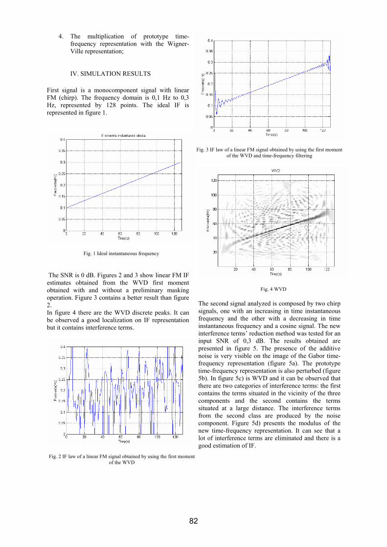
4. The multiplication of prototype time-frequency representation with the Wigner-Ville representation;

IV. SIMULATION RESULTS First signal is a monocomponent signal with linear FM (chirp). The frequency domain is 0,1 Hz to 0,3 Hz, represented by 128 points. The ideal IF is represented in figure 1.

Fig. 1 Ideal instantaneous frequency The SNR is 0 dB. Figures 2 and 3 show linear FM IF estimates obtained from the WVD first moment obtained with and without a preliminary masking operation. Figure 3 contains a better result than figure 2. In figure 4 there are the WVD discrete peaks. It can be observed a good localization on IF representation but it contains interference terms.

Fig. 2 IF law of a linear FM signal obtained by using the first moment of the WVD

Fig. 3 IF law of a linear FM signal obtained by using the first moment of the WVD and time-frequency filtering

Fig. 4 WVD The second signal analyzed is composed by two chirp signals, one with an increasing in time instantaneous frequency and the other with a decreasing in time instantaneous frequency and a cosine signal. The new interference terms’ reduction method was tested for an input SNR of 0,3 dB. The results obtained are presented in figure 5. The presence of the additive noise is very visible on the image of the Gabor time-frequency representation (figure 5a). The prototype time-frequency representation is also perturbed (figure 5b). In figure 5c) is WVD and it can be observed that there are two categories of interference terms: the first contains the terms situated in the vicinity of the three components and the second contains the terms situated at a large distance. The interference terms from the second class are produced by the noise component. Figure 5d) presents the modulus of the new time-frequency representation. It can see that a lot of interference terms are eliminated and there is a good estimation of IF.

82

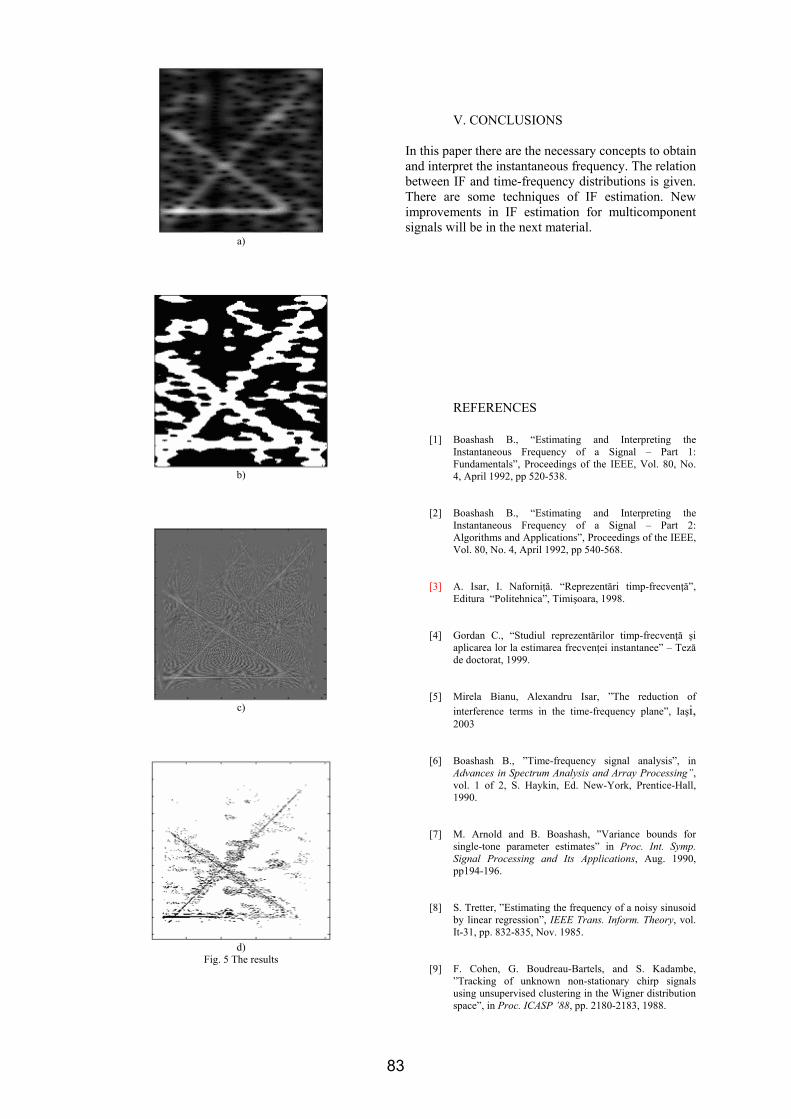
a)

b)

c)

d)

Fig. 5 The results

V. CONCLUSIONS

In this paper there are the necessary concepts to obtain and interpret the instantaneous frequency. The relation between IF and time-frequency distributions is given. There are some techniques of IF estimation. New improvements in IF estimation for multicomponent signals will be in the next material. REFERENCES

[1] Boashash B., “Estimating and Interpreting the Instantaneous Frequency of a Signal – Part 1: Fundamentals”, Proceedings of the IEEE, Vol. 80, No. 4, April 1992, pp 520-538.

[2] Boashash B., “Estimating and Interpreting the

Instantaneous Frequency of a Signal – Part 2: Algorithms and Applications”, Proceedings of the IEEE, Vol. 80, No. 4, April 1992, pp 540-568.

[3] A. Isar, I. Naforniţă. “Reprezentări timp-frecvenţă”, Editura “Politehnica”, Timişoara, 1998.

[4] Gordan C., “Studiul reprezentărilor timp-frecvenţă şi aplicarea lor la estimarea frecvenţei instantanee” – Teză de doctorat, 1999.

[5] Mirela Bianu, Alexandru Isar, ”The reduction of

interference terms in the time-frequency plane”, Iaşi, 2003

[6] Boashash B., ”Time-frequency signal analysis”, in

Advances in Spectrum Analysis and Array Processing”, vol. 1 of 2, S. Haykin, Ed. New-York, Prentice-Hall, 1990.

[7] M. Arnold and B. Boashash, ”Variance bounds for

single-tone parameter estimates” in Proc. Int. Symp. Signal Processing and Its Applications, Aug. 1990, pp194-196.

[8] S. Tretter, ”Estimating the frequency of a noisy sinusoid

by linear regression”, IEEE Trans. Inform. Theory, vol. It-31, pp. 832-835, Nov. 1985.

[9] F. Cohen, G. Boudreau-Bartels, and S. Kadambe,

”Tracking of unknown non-stationary chirp signals using unsupervised clustering in the Wigner distribution space”, in Proc. ICASP ’88, pp. 2180-2183, 1988.

83

[10] Boashash B., B. Lovell and P. Kootsookos, ”Time-frequency signal analysis and instantaneous frequency: their inter-relationship and applications”, presented at the Proc. ISCAS, OR, Apr. 1989.

[11] Y. Zhao, L. E. Atlas, “The use of coneshape kernels for

generalized time-frequency representation of non-stationary signals”, IEEE Transactions on Acoustics, Speech, and Signal Processing, June, 1990.

84

Buletinul Ştiinţific al Universităţii “Politehnica” din Timişoara

Seria ELECTRONICĂ şi TELECOMUNICAŢII TRANSACTIONS on ELECTRONICS and COMMUNICATIONS

Tom 48 (62), Fascicola 1, 2003

Doppler Signal Extractor

Dan Gh. T. POPA Abstract - The paper presents a technical solution, proposed by the author, for extracting the Doppler signal in a Doppler telemetry system with active fixed referential. The role of the presented electronic circuits is to center the Doppler shift in frequency, in order to establish the motion sense of the mobile and to select a sin or cosin signal that contains in its argument only the Doppler shift in frequency. In this way, the extracted Doppler signal allows the evaluation of the mobile movement by speed, position and direction. Key words: Doppler shift in frequency, centering of the Doppler shift in frequency, Doppler telemetry system with active fixed referential.

I. INTRODUCTION When evaluating motion with low speed and low costs, we have to use a cheap Doppler telemetry system in order to extract the Doppler signal resulting from the movement of the considered mobile. For that, the author proposes activation of the fixed referential as well as a structure with active fixed referential for the Doppler telemetry system [4], [5]. The electronic equipment on the mobile referential is receiving the signal sr2(

'2ω ) and can make use of

the signal s2(ω2), that is synchronous with the received signal, defined by relations: s2(ω2) = A2 sin(ω2t + φ) (1) sr2(

'2ω ) = Ar2 sin(ω2t + ωjt ± 2∆ω2t + φ) +

+ Ar2 sin(ω2t - ωjt ± 2∆ω2t + φ) (2) where '

2ω = ω2 ± ωj ± ∆ω2 (3)

It can be clearly seen that the Doppler information ∆ω2 is contained by the signal sr2 through the argument '

2ω . The circuit to extract the Doppler signal has to realize the following functions: a) elimination of the carrier ω2; b) centering of the Doppler shift in frequency, in order to establish the motion sense for the mobile referential versus the fixed one;

c) to reject the pulse ωj and to generate a sin or cosin signal, to contain in its argument only the Doppler shift in frequency. The low frequency fj has been introduced in order to realise the centering of the Doppler shift in frequency and its separation [4], [5]. Following the presented considerations, the Doppler signal is: - the signal that contains in its argument only ωj and the Doppler shift in frequency ± ∆ω2, allowing the determination of the motion sense of the mobile referential versus the active fixed one; - the signal that contains in its argument only the Doppler shift in frequency, that allows determination of the movement speed for the mobile referential. In order to realize the three functions, the structure presented in Fig. 1 is proposed. It is conceived with professional electronic circuits.

II. ELIMINATION OF THE ω2 CARRIER The M1 and M2 modulators, together with the dephasing circuit with π/2, are forming a pair of quadrature modulators with suppression of the carrier [2], [3]. The M1 modulator, together with the active filter AF1 (low-pass type) and the M2 modulator, together with the active filter AF2 are forming the SSB-SC modulators, with the selection of the lower sideband (the difference between the carrier pulsation and the modulating pulsation). Under these conditions, the signal '

1ms is obtained

by multiplication of the sr2('2ω ) and s2(ω2) signal,

having the form:

tAA

tAAs

jr

jrm

)2cos(21

)2cos(21

222

222'

1

ωω

ωω

∆±−+

+∆±= (4)

85

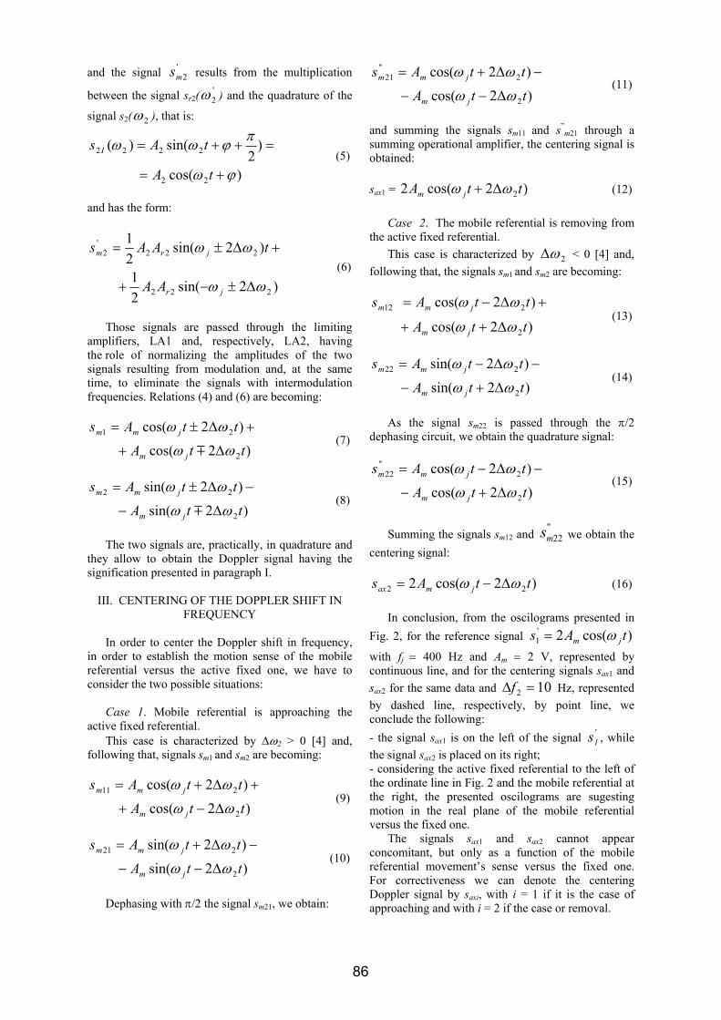
and the signal '2ms results from the multiplication

between the signal sr2('2ω ) and the quadrature of the

signal s2( 2ω ), that is:

)cos(

)2

sin()(

22

2222

ϕω

πϕωω

+=

=++=

tA

tAs I (5)

and has the form:

)2sin(21

)2sin(21

222

222'

2

ωω

ωω

∆±−+

+∆±=

jr

jrm

AA

tAAs (6)

Those signals are passed through the limiting amplifiers, LA1 and, respectively, LA2, having the role of normalizing the amplitudes of the two signals resulting from modulation and, at the same time, to eliminate the signals with intermodulation frequencies. Relations (4) and (6) are becoming:

)2cos(

)2cos(

2

21

ttA

ttAs

jm

jmm

ωω

ωω

∆+

+∆±=

m (7)

)2sin(

)2sin(

2

22

ttA

ttAs

jm

jmm

ωω

ωω

∆−

−∆±=

m (8)

The two signals are, practically, in quadrature and they allow to obtain the Doppler signal having the signification presented in paragraph I.

III. CENTERING OF THE DOPPLER SHIFT IN FREQUENCY

In order to center the Doppler shift in frequency, in order to establish the motion sense of the mobile referential versus the active fixed one, we have to consider the two possible situations: Case 1. Mobile referential is approaching the active fixed referential. This case is characterized by ∆ω2 > 0 [4] and, following that, signals sm1 and sm2 are becoming:

)2cos(

)2cos(

2

211

ttA

ttAs

jm

jmm

ωω

ωω

∆−+

+∆+= (9)

)2sin(

)2sin(

2

221

ttA

ttAs

jm

jmm

ωω

ωω

∆−−

−∆+= (10)

Dephasing with π/2 the signal sm21, we obtain:

)2cos(

)2cos(

2

2"

21

ttA

ttAs

jm

jmm

ωω

ωω

∆−−

−∆+= (11)

and summing the signals sm11 and s”

m21 through a summing operational amplifier, the centering signal is obtained: sax1 = )2cos(2 2ttA jm ωω ∆+ (12) Case 2. The mobile referential is removing from the active fixed referential. This case is characterized by 2ω∆ < 0 [4] and, following that, the signals sm1 and sm2 are becoming:

)2cos(

)2cos(

2

212

ttA

ttAs

jm

jmm

ωω

ωω

∆++

+∆−= (13)

)2sin(

)2sin(

2

222

ttA

ttAs

jm

jmm

ωω

ωω

∆+−

−∆−= (14)

As the signal sm22 is passed through the π/2 dephasing circuit, we obtain the quadrature signal:

)2cos(

)2cos(

2

2"

22

ttA

ttAs

jm

jmm

ωω

ωω

∆+−

−∆−= (15)

Summing the signals sm12 and "

22ms we obtain the centering signal:

)2cos(2 22 ttAs jmax ωω ∆−= (16) In conclusion, from the oscilograms presented in Fig. 2, for the reference signal )cos(2'

1 tAs jm ω=

with fj = 400 Hz and Am = 2 V, represented by continuous line, and for the centering signals sax1 and sax2 for the same data and 102 =∆f Hz, represented by dashed line, respectively, by point line, we conclude the following: - the signal sax1 is on the left of the signal '

1s , while the signal sax2 is placed on its right; - considering the active fixed referential to the left of the ordinate line in Fig. 2 and the mobile referential at the right, the presented oscilograms are sugesting motion in the real plane of the mobile referential versus the fixed one. The signals sax1 and sax2 cannot appear concomitant, but only as a function of the mobile referential movement’s sense versus the fixed one. For correctiveness we can denote the centering Doppler signal by saxi, with i = 1 if it is the case of approaching and with i = 2 if the case or removal.

86

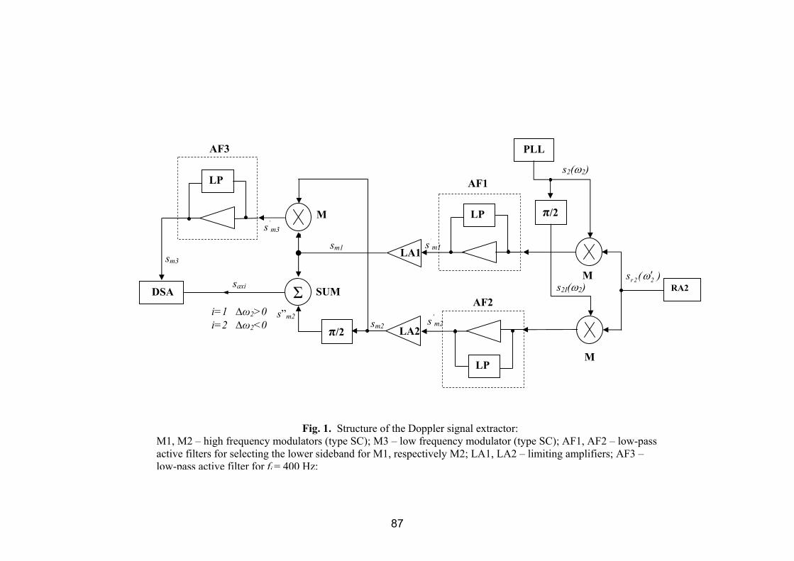
RA2 )(s 22r ω′

Fig. 1. Structure of the Doppler signal extractor: M1, M2 – high frequency modulators (type SC); M3 – low frequency modulator (type SC); AF1, AF2 – low-pass active filters for selecting the lower sideband for M1, respectively M2; LA1, LA2 – limiting amplifiers; AF3 – low-pass active filter for fj = 400 Hz;

LP

DSA Σ

π/2

LP

LP

LA1

LA2

π/2

PLL

sm3

saxi

sm1

s’m3

M

SUM

M

M

AF3

AF1

AF2i=1 ∆ω2>0i=2 ∆ω2<0

s2(ω2)

s2I(ω2)

s’m1

s’m2 sm2

s”m2

87

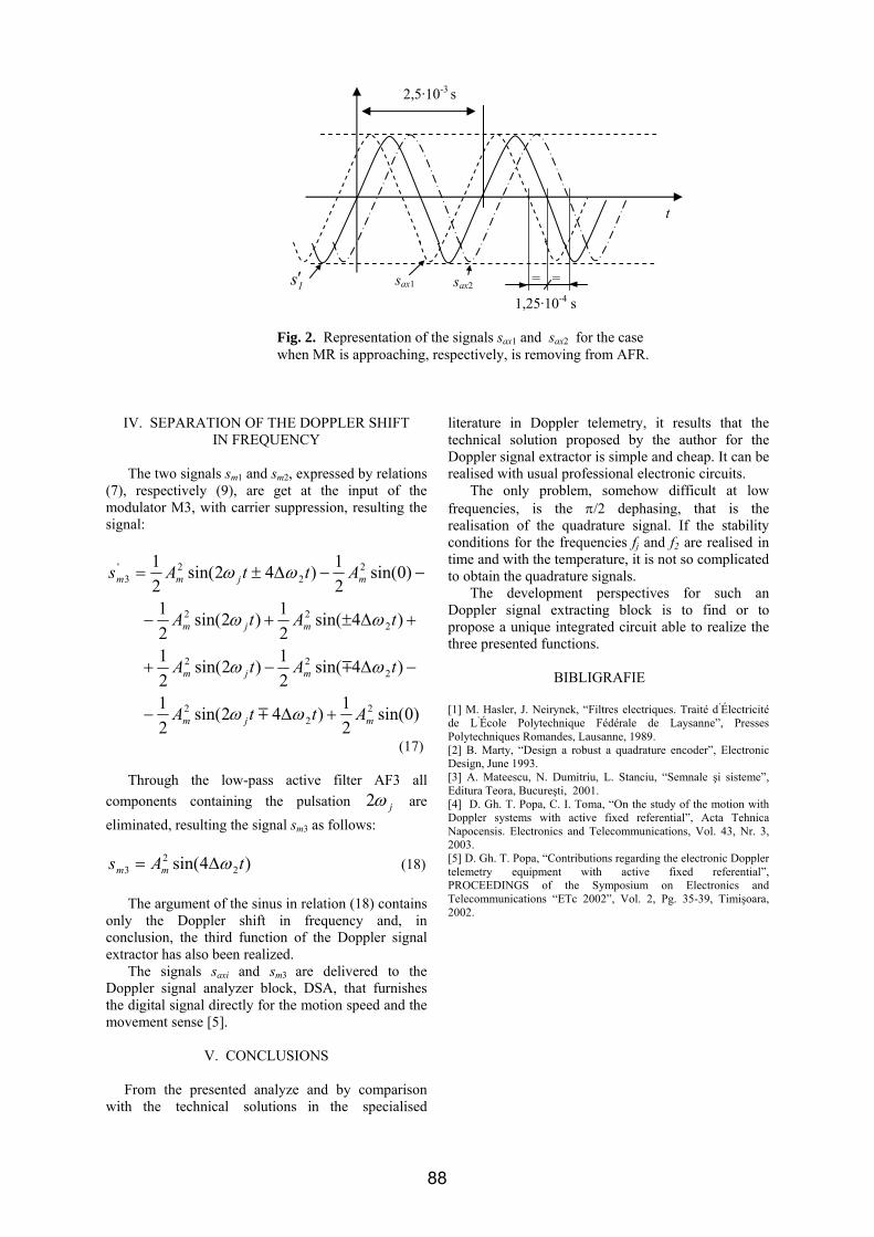
IV. SEPARATION OF THE DOPPLER SHIFT IN FREQUENCY

The two signals sm1 and sm2, expressed by relations (7), respectively (9), are get at the input of the modulator M3, with carrier suppression, resulting the signal:

)0sin(21)42sin(

21

)4sin(21)2sin(

21

)4sin(21)2sin(

21

)0sin(21)42sin(

21

22

2

222

222

22

2'3

mjm

mjm

mjm

mjmm

AttA

tAtA

tAtA

AttAs

+∆−

−∆−+

+∆±+−

−−∆±=

ωω

ωω

ωω

ωω

m

m

(17) Through the low-pass active filter AF3 all components containing the pulsation jω2 are eliminated, resulting the signal sm3 as follows:

)4sin( 22

3 tAs mm ω∆= (18) The argument of the sinus in relation (18) contains only the Doppler shift in frequency and, in conclusion, the third function of the Doppler signal extractor has also been realized. The signals saxi and sm3 are delivered to the Doppler signal analyzer block, DSA, that furnishes the digital signal directly for the motion speed and the movement sense [5].

V. CONCLUSIONS

From the presented analyze and by comparison with the technical solutions in the specialised

literature in Doppler telemetry, it results that the technical solution proposed by the author for the Doppler signal extractor is simple and cheap. It can be realised with usual professional electronic circuits. The only problem, somehow difficult at low frequencies, is the π/2 dephasing, that is the realisation of the quadrature signal. If the stability conditions for the frequencies fj and f2 are realised in time and with the temperature, it is not so complicated to obtain the quadrature signals. The development perspectives for such an Doppler signal extracting block is to find or to propose a unique integrated circuit able to realize the three presented functions. BIBLIGRAFIE [1] M. Hasler, J. Neirynek, “Filtres electriques. Traité d’Électricité de L’École Polytechnique Fédérale de Laysanne”, Presses Polytechniques Romandes, Lausanne, 1989. [2] B. Marty, “Design a robust a quadrature encoder”, Electronic Design, June 1993. [3] A. Mateescu, N. Dumitriu, L. Stanciu, “Semnale şi sisteme”, Editura Teora, Bucureşti, 2001. [4] D. Gh. T. Popa, C. I. Toma, “On the study of the motion with Doppler systems with active fixed referential”, Acta Tehnica Napocensis. Electronics and Telecommunications, Vol. 43, Nr. 3, 2003. [5] D. Gh. T. Popa, “Contributions regarding the electronic Doppler telemetry equipment with active fixed referential”, PROCEEDINGS of the Symposium on Electronics and Telecommunications “ETc 2002”, Vol. 2, Pg. 35-39, Timişoara, 2002.

t

2,5·10-3 s

sax1 sax2 1s′ = =

1,25·10-4 s

Fig. 2. Representation of the signals sax1 and sax2 for the case when MR is approaching, respectively, is removing from AFR.

88

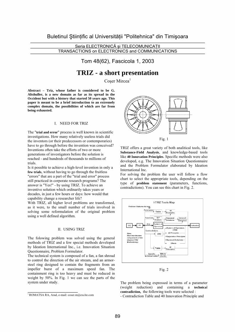
Buletinul Ştiinţific al Universităţii "Politehnica" din Timişoara

Seria ELECTRONICĂ şi TELECOMUNICAŢII TRANSACTIONS on ELECTRONICS and COMMUNICATIONS

Tom 48(62), Fascicola 1, 2003

TRIZ - a short presentation

Coşer Mircea1

Abstract – Triz, whose father is considered to be G. Altshuller, is a new domain as far as its spread in the Occident but with a history that started 50 years ago. This paper is meant to be a brief introduction to an extremely complex domain, the possibilities of which are far from being exhausted.

I. NEED FOR TRIZ

The "trial and error" process is well known in scientific investigations. How many relatively useless trials did the inventors (or their predecessors or contemporaries) have to go through before the invention was conceived? Inventions often take the efforts of two or more generations of investigators before the solution is reached - and hundreds of thousands to millions of trials. Is it possible to achieve a high-level invention in only a few trials, without having to go through the fruitless "errors" that are a part of the "trial and error" process still practiced in corporate research programs? The answer is "Yes!" - by using TRIZ. To achieve an inventive solution which ordinarily takes years or decades, in just a few hours or days: how would that capability change a researcher life? With TRIZ, all higher level problems are transformed, as it were, to the small number of trials involved in solving some reformulation of the original problem using a well defined algorithm.

II. USING TRIZ The folowing problem was solved using the general methods of TRIZ and a few special methods developed by Ideation International Inc., i.e. Innovation Situation Questionnaire, Problem Formulator. The technical system is composed of a fan, a fan shroud to control the direction of the air stream, and an armor-steel ring designed to contain the fragments from an impeller burst of a maximum speed fan. The containment ring is too heavy and must be reduced in weight by 50%. In Fig. 1 we can see the parts of the system under study. 1 ROMATSA RA, Arad, e-mail: coser.m@excite.com

Fig. 1 TRIZ offers a great variety of both analitical tools, like Substance-Field Analysis, and knowledge-based tools like 40 Innovation Principles. Specific methods were also developed, e.g. The Innovation Situation Questionnaire and the Problem Formulator elaborated by Ideation International Inc. For solving the problem the user will follow a flow chart to select the appropriate tools, depending on the type of problem statement (parameters, functions, contradictions). You can see this chart in Fig. 2.

Fig. 2

The problem being expressed in terms of a parameter (weight reduction) and containing a technical contradiction, the following tools were selected : - Contradiction Table and 40 Innovation Principle and

89

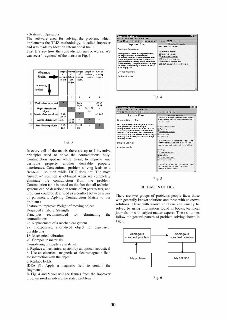
- System of Operators The software used for solving the problem, which implements the TRIZ methodology, is called Improver and was made by Ideation International Inc. I First let's see how the contradiction matrix works. We can see a "fragment" of the matrix in Fig. 3

Fig. 3

In every cell of the matrix there are up to 4 inventive principles used to solve the contradictions fully. Contradiction appears while trying to improve one desirable property another desirable property deteriorates. Conventional problem solving leads to a "trade-off" solution while TRIZ does not. The most "inventive" solution is obtained when we completely eliminate the contradiction from the problem. Contradiction table is based on the fact that all technical systems can be described in terms of 39 parameters, and problems could be described as a conflict between a pair of parameters. Aplying Contradiction Matrix to our problem : Feature to improve: Weight of moving object Degraded attribute: Strength Principles recommended for eliminating the contradiction: 28. Replacement of a mechanical system 27. Inexpensive, short-lived object for expensive, durable one 18. Mechanical vibration 40. Composite materials Considering principle 28 in detail: a. Replace a mechanical system by an optical, acoustical b. Use an electrical, magnetic or electromagnetic field for interaction with the object c. Replace fields IDEA #1: Apply a magnetic field to contain the fragments. In Fig. 4 and 5 you will see frames from the Improver program used in solving the stated problem.

Fig. 4

Fig. 5

III. BASICS OF TRIZ

There are two groups of problems people face: those with generally known solutions and those with unknown solutions. Those with known solutions can usually be solved by using information found in books, technical journals, or with subject matter experts. These solutions follow the general pattern of problem solving shown in Fig. 6

Fig. 6

Analogous

standard problem

Analogous

standard solution

My problem

My solution

90

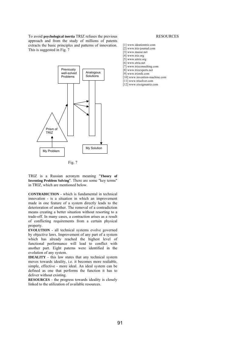
To avoid psychological inertia TRIZ refuses the previous approach and from the study of millions of patents extracts the basic principles and patterns of innovation. This is suggested in Fig. 7

Fig. 7 TRIZ is a Russian acronym meaning "Theory of Inventing Problem Solving". There are some "key terms" in TRIZ, which are mentioned below. CONTRADICTION - which is fundamental in technical innovation - is a situation in which an improvement made in one feature of a system directly leads to the deterioration of another. The removal of a contradiction means creating a better situation without resorting to a trade-off. In many cases, a contraction arises as a result of conflicting requirements from a certain physical property. EVOLUTION - all technical systems evolve governed by objective laws. Improvement of any part of a system which has already reached the highest level of functional performance will lead to conflict with another part. Eight paterns were identified in the evolution of any system. IDEALITY - this law states that any technical system moves towards ideality, i.e. it becomes more realiable, simple, effective - more ideal. An ideal system can be defined as one that performs the function it has to deliver without existing. RESOURCES - the progress towards ideality is closely linked to the utilization of available resources.

RESOURCES

[1] www.ideationtriz.com [2] www.triz-journal.com [3] www.mazur.net [4] www.triz.org [5] www.aitriz.org [6] www.etria.net [7] www.trizconsulting.com [8] www.trizexperts.net [9] www.triznik.com [10] www.invention-machine.com [11] www.trisolver.com [12] www.sixsigmatriz.com

My Problem My Solution

Prism of TRIZ

Analogous Solutions

Previously well-solved Problems

91

Buletinul Ştiinţific al Universităţii "Politehnica" din Timişoara

Seria ELECTRONICĂ şi TELECOMUNICAŢII TRANSACTIONS on ELECTRONICS and COMMUNICATIONS

Tom 48(62), Fascicola 2, 2003

Instrucţiuni de redactare a articolelor pentru Buletinul ştiinţific al Facultăţii de Electronică şi Telecomunicaţii

Gheorghe I. Popescu1

1 Facultatea de Electronică şi Telecomunicaţii, Departamentul Comunicaţii Bd. V. Pârvan Timişoara 1900 e-mail geo@ee.utt.ro

Rezumat – Aceste instrucţiuni sunt concepute să vă prezinte modul de redactare al articolelor pentru Buletinul ştiinţific al Facultăţii de Electronică şi Telecomunicaţii. Prezentul material este conceput ca model pentru modul cum trebuie să arate articolele gata de publicare. Rezumatul trebuie să conţină descrierea problemei, metodele şi soluţiile propuse şi rezultatele experimentale obţinute în cel mult 12 rânduri. Nu se admit referinţe bibliografice în cadrul rezumatului. Cuvinte cheie: redactare, buletin ştiinţific

I. INTRODUCERE

Formatul buletinului va fi A4. Articolele, inclusiv tabelele şi figurile, nu trebuie să depăşească 6 pagini. Numărul de pagini trebuie să fie obligatoriu par.

II. INSTRUCŢIUNI DE REDACTARE

Articolul trebuie să fie transmis în forma standard descrisă în acest material. Tipărirea se va face cu o imprimantă de bună calitate pe o singură faţă a paginii. Textul se va plasa pe două coloane de 8 cm cu spaţiu de 0,5 cm între ele. Pagina A4 orientată pe înălţimea paginii are marginile de sus şi jos de 1,78 cm, iar cele din stânga şi dreapta de 2,54 cm. Prima pagină a articolului va avea marginea superioară de 5 cm. Pentru editarea articolului se recomandă utilizarea procesorului de text Microsoft Word for Windows cu caractere Times New Roman dactilografiate la un rând. Dimensiunile şi stilul caracterelor sunt: Titlul articolului 18 pt îngroşat, autorul 12 pt rezumatul 9 pt îngroşat, cuvintele cheie 9 pt îngroşat, titlu paragraf 10 pt majuscule, titlu subparagraf 10 pt italic, distanţa de la numărul de ordine la titluri va fi de 0,25 cm, textul normal 10 pt, afilierea autorului 8 pt, notele de subsol 8 pt, legendele figurilor 8 pt şi bibliografia 8 pt.

III. FIGURI ŞI TABELE Figurile şi tabelele trebuiesc inserate în text aliniate la stânga. Se recomandă evitarea plasării figurilor înainte de prima lor menţionare în text. Se va folosi abrevierea “Fig.1.” chiar şi la începutul propoziţiilor. Ecuaţiile

trebuie tipărite cu un rând gol deasupra şi dedesubt. Numerotarea lor se face simplu în paranteze: (1), (2), (3) … Numerotarea va fi aliniată faţă de marginea dreaptă.

IV. REFERINŢE BIBLIOGRAFICE Referinţele bibliografice se numerotează consecutiv în forma [1], [2], [3]… Citările se fac simplu prin plasarea numărului corespunzător [5]. Nu sunt permise referinţe bibliografice în notele de referinţă în subsol. Se recomandă scrierea tuturor autorilor şi nu folosirea expresiei “şi alţii” decât dacă sunt peste 6 autori.

V. SFATURI UTILE A. Abrevieri şi acronime Explicitaţi abrevierile şi acronimele prima dată când ele apar în text. Abrevieri precum IEEE, IEE, SI, MKS, CGS, ac, dc şi rms se consideră cunoscute şi nu mai trebuie explicitate. Nu se recomandă utilizarea abrevierilor în titluri decât în cazul când sunt absolut inevitabile. B. Alte recomandări Se recomandă utilizarea unităţilor de măsură din sistemul internaţional. Utilizarea unităţilor britanice poate fi făcută doar ca unităţi secundare (în paranteză). Se va evita combinarea unităţilor SI şi CGS. Nu se admit rezultate experimentale preliminare. Numerotarea cu cifre romane a titlurilor de paragrafe este opţională. În cazul utilizării acestora se vor numerota paragrafelor propriu-zise şi nu “BIBLIOGRAFIA” sau “MULŢUMIRI”.

BIBLIOGRAFIE [1] A. Ignea, “Preparation of papers for the International Sympozium Etc. ’98”, Buletinul Universităţii “Politehnica” Tom 43 (57), 1998, Fascicola 1, 1998, pp. 81